HAL Id: hal-00329406
https://hal.archives-ouvertes.fr/hal-00329406
Submitted on 3 Jun 2005
HAL is a multi-disciplinary open access
archive for the deposit and dissemination of
sci-entific research documents, whether they are
pub-lished or not. The documents may come from
teaching and research institutions in France or
abroad, or from public or private research centers.
L’archive ouverte pluridisciplinaire HAL, est
destinée au dépôt et à la diffusion de documents
scientifiques de niveau recherche, publiés ou non,
émanant des établissements d’enseignement et de
recherche français ou étrangers, des laboratoires
publics ou privés.
boundary layer
G. Paschmann, S. Haaland, B. U. Ö. Sonnerup, H. Hasegawa, E. Georgescu,
B. Klecker, T. D. Phan, H. Rème, A. Vaivads
To cite this version:
G. Paschmann, S. Haaland, B. U. Ö. Sonnerup, H. Hasegawa, E. Georgescu, et al.. Characteristics of
the near-tail dawn magnetopause and boundary layer. Annales Geophysicae, European Geosciences
Union, 2005, 23 (4), pp.1481-1497. �hal-00329406�
SRef-ID: 1432-0576/ag/2005-23-1481 © European Geosciences Union 2005
Annales
Geophysicae
Characteristics of the near-tail dawn magnetopause and boundary
layer
G. Paschmann1, S. Haaland1, B. U. ¨O. Sonnerup2, H. Hasegawa2, E. Georgescu1, B. Klecker1, T. D. Phan3, H. R`eme4,
and A. Vaivads5
1Max-Planck-Institut f¨ur extraterrestrische Physik, Garching, Germany 2Thayer School of Engineering, Dartmouth College, Hanover, NH, USA 3Space Sciences Laboratory, University of California, Berkeley, CA, USA 4CESR-CNRS, Toulouse, France
5Swedish Institute of Space Physics, Uppsala, Sweden
Received: 1 February 2005 – Revised: 29 March 2005 – Accepted: 31 March 2005 – Published: 3 June 2005
Abstract. The paper discusses properties of the near-tail
dawnside magnetopause and boundary layer, as obtained from Cluster plasma and magnetic field measurements dur-ing a sdur-ingle skimmdur-ing orbit on 4 and 5 July 2001 that in-cluded 24 well-defined magnetopause crossings by all four spacecraft. As a result of variations of the interplanetary magnetic field, the magnetic shear across the local magne-topause varied between ∼0◦and ∼180◦. Using an improved
method, which takes into account magnetopause accelera-tion and thickness variaaccelera-tion, we have determined the magne-topause orientation, speed, thickness and current for the 96 individual magnetopause crossings. The orientations show clear evidence of surface waves. Magnetopause thicknesses range from ∼100 to ∼2500 km, with an average of 753 km. The magnetopause speeds range from less than 10 km s−1up to more than 300 km s−1, with an average of 48 km s−1. Both results are consistent with earlier ISEE and AMPTE results obtained for the dayside magnetopause. Importantly, scal-ing the thicknesses to the ion gyro radius or the ion inertial length did not reduce the large dynamic range. There is also no significant dependence of thickness on magnetic shear. Current densities range from ∼0.01 µA m−2 up to ∼0.3 uA, with an average value of 0.05 µA m−2. By including some extra crossings that did not involve all four spacecraft, we were able to apply the Wal´en test to a total of 60 crossings by Cluster 1 and 3, and have classified 19 cases as rotational discontinuities (RDs), of which 12 and 7 were crossings sun-ward and tailsun-ward of an X-line, respectively. Of these 60 crossings, 26 show no trace of a boundary layer. The only crossings with substantial boundary layers are crossings into the plasma mantle. Of the 26 crossings without a bound-ary layer, 8 were identified as RDs. Since reconnection pro-duces wedge-shaped boundary layers emanating from the X-line, RDs without boundary layer may be considered
cross-Correspondence to: G. Paschmann
(goetz.paschmann@mpe.mpg.de)
ings close to the X-line, in which case the observed magnetic shear and Alfv´en Mach number should be representative of the conditions at the X-line itself. It is therefore important that four of the eight cases had shear angles ≤100◦, i.e. the reconnecting fields were far from being anti-parallel, and that all eight cases had Alfv´en Mach numbers MA>1 in the
ad-joining magnetosheath. Another important conclusion can be drawn from the crossings without a boundary layer that were tangential discontinuities (TDs). To observe TDs with no boundary layer at such large distances from the subso-lar point appears to rule out diffusion over subso-large portions of the magnetopause as an effective means for plasma transport across the magnetopause.
Key words. Magnetospheric physics (Magnetopause, cusp
and boundary layers; Solar wind-magnetosphere interac-tions) – Space plasma physics (magnetic reconnection)
1 Introduction
This paper discusses properties of the near-tail dawnside magnetopause and boundary layer as obtained from plasma and magnetic field measurements by the Cluster spacecraft during a single skimming orbit that included 24 well-defined crossings by all four spacecraft. Emphasis is placed on de-terminations of the magnetopause orientation, speed, thick-ness, and currents; on magnetopause classification in terms of tangential vs. rotational discontinuity; separation of the crossings into those with and without an adjoining bound-ary layer; investigation of the magnetic shear dependence of magnetopause and boundary layer properties; and the identi-fication of surface waves.
We use vector magnetic field measurements obtained by the flux gate magnetometer instrument FGM on all four spacecraft (Balogh et al., 1997). For overview purposes we present the data in terms of the standard 4-s spin-resolution
1482 G. Paschmann et al.: The dawnside magnetopause and boundary layer -10 10 -10 10 23:57 UT 17:27 UT XGSE YGSE -10 10 ZGSE -10 10 YGSE 17:27 UT 23:57 UT a) b) 1 2 13 20 21 29 c) d) e) -5 0 B_IMF [nT] -100 0 100 Phi [deg] 2300 0000 0100 0200 0300 0400 0500 0600 0700 0800 0900 1000 1100 1200 1300 1400 1500 1600 1700 1800 0.1 1.0 10.0 100.0 Np [1/cm 3] -5 0 5 Bx [nT] -5 0 5 By [nT] -5 0 5 Bz [nT] -100 0 100 Φ [deg] 2300 0000 0100 0200 0300 0400 0500 0600 0700 0800 0900 1000 1100 1200 1300 1400 1500 1600 1700 1800 0.1 1.0 10.0 100.0 Np [1/cm 3]
Fig. 1. Overview of spacecraft position and key parameters. Top: GSE XY (a) and YZ (b) projections of spacecraft orbit. The spacecraft
separation distances are magnified by a factor of ∼5 to show the tetrahedron configuration. The thick black lines show the trajectory during the time interval discussed in this paper. Panels (c): the three components of the IMF measured at ACE, shifted to account for the propagation delay. Panel (d): magnetic field orientation observed at Cluster C1. The angle φ is the azimuth angle in the (L,M)-plane of the boundary-normal coordinate system; φ=0◦is along the L-axis, which is pointing essentially northward. φ=90◦is along the M axis, which is pointing tailward along the magnetopause. Panel (e): plasma density from the CIS HIA instrument on C1. The labelled crossings (blue for inbound, red for outbound) are discussed in Sect. 5
.
averages, but for detailed analysis we use 0.2-s averages. For the plasma properties we use the standard 4-s spin-resolution moments (density, bulk velocity, temperature) calculated on board from the 3-D ion distribution functions measured by CIS-HIA on spacecraft C1 and C3 (R`eme et al., 2001). We also use the 0.2-s resolution electron densities inferred from the spacecraft potential measurements by the EFW instru-ment (Gustafsson et al., 1997).
2 Overview
Between 23:40 UT on 4 July and 17:40 UT on 5 July 2001, the Cluster satellites were skimming the near-tail dawnside magnetopause at local times between 5.0 and 3.8 h and at
lat-itudes decreasing from 32◦to 4◦(in GSM coordinates). The spacecraft separation distances were ∼3000 km at the begin-ning and ∼2000 km at the end of this time interval. Figure 1 shows the orbit and an overview of the interval, with inter-planetary magnetic field (IMF) data from ACE, and magnetic field and plasma density from Cluster C1. Magnetopause crossings are recognized by a magnetic field rotation (panel d) and a jump in the ion density, from typical values of 10 to 20 cm−3in the magnetosheath to values <1 cm−3in the magnetosphere (panel e).
Cluster first encountered the magnetopause around 23:57 UT on 4 July. The last crossing included in this study took place around 17:27 UT on 5 July. There were a total of 24 well-defined four-spacecraft crossings in this interval,
of which 13 were outbound crossings, and 11 were inbound crossings. In addition, there were several crossings that did not involve all spacecraft. Numbers along the bottom panel of Fig. 1 mark the crossing number of the six magnetopause encounters presented in detail in Sect. 5. Note that the cross-ing at 06:23 UT, not dicussed here in detail, has already been the subject of several studies (Haaland et al., 2004; Hasegawa et al., 2004a,b).
As seen in Fig. 1, the interplanetary magnetic field mea-sured by ACE, (panels c), was highly variable, particularly the north-south (i.e. Bz) component. The solar wind dynamic
pressure (not shown), on the other hand, remained nearly constant at 2.5 nPa, with maxima and minima near 3.5 and 1.5 nPa, respectively. There is a tendency for the spacecraft to remain in the magnetosheath for longer periods for higher values of the dynamic pressure, when, based on pressure bal-ance, the magnetopause is expected to be pushed in further. As we will see later, there is also clear evidence for crossings being caused by surface undulations.
Figure 1d shows the measured field direction, φ, at C1 in the (L, M)-plane of the boundary normal cordinate system, where L and M point essentially northward, and tailward, re-spectively, in the plane tangent to the (model) magnetopause, with φ being counted from the L axis. The magnetic field on the magnetospheric side of the magnetopause was stable over the entire time interval and directed essentially along the negative M direction, as identified by φ-angles near −90◦in
Fig. 1d. This is the expected direction for tailward stretched field lines in the Northern Hemisphere. In response to the variable IMF, the field direction in the magnetosheath was quite variable, as illustrated by the strong variations in φ, including fields directed anti-parallel to the magnetospheric field, φ=90◦, as shown in panel (d). The translation from the measured IMF at ACE to the magnetosheath field adja-cent to the magnetopause crossings is, however, by no means straightforward, as it involves draping of the field around the magnetospheric obstacle, and its temporal response when the IMF, especially its Bycomponent, changes.
From high-resolution plots of the φ angle, the sense and magnitude of the rotation of the field across the magne-topause (i.e. the magnetic shear angle) could be unambigu-ously determined. We quantify the shear by the (signed) change in φ relative to the magnetospheric orientation. The shear is counted positive if φ changes towards more positive values; it is negative for a change in the more negative direc-tion. With this definition, the magnitude of the shear could, in principle, exceed 180◦. It is thus significant that no shear angles with magnitude >180◦have been observed, confirm-ing the result reported by Berchem and Russell (1982) that the field rotation across the magnetopause has no preferred sense, but always takes the shortest path.
3 Four-spacecraft analysis
For each of the 24 complete crossings, we calculated magne-topause orientation, velocity, thickness, and current density.
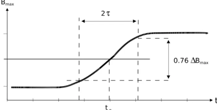
0.76∆Bmax
Bmax
t 2τ
t 0
Fig. 2. Our definition of crossing time, t0, and crossing duration, 2 τ
for a Harris sheet-like profile of Bmax. With a known magnetopause
velocity, VMP, the magnetopause thickness, dMP is given by 2τ ∗
VMP.
The basic procedure involved the following steps:
– Perform variance analysis of the spin resolution
mag-netic field from each spacecraft to establish a new coor-dinate system, defined by the eigenvectors of the vari-ance matrix. Use the rotation matrix from the best of these results, and rotate the high-resolution (0.2 s) mag-netic field from all spacecraft into the same local bound-ary normal coordinate system.
– Identify relative crossing time, crossing duration and
B-field jump for each spacecraft from profiles of the max-imum variance components.
– Apply the multi-spacecraft method described below to
determine magnetopause orientation, motion and thick-ness at each spacecraft.
– Use the observed magnetic field jump and the calculated
thickness to estimate the current density at each space-craft.
3.1 Timing procedure
In its simplest form, a multi-spacecraft determination of magnetopause orientation and motion makes use of the mea-sured differences in crossing time and the known separation vectors between the spacecraft. The magnetopause thickness is thereafter calculated from the crossing duration and veloc-ity. In order to determine the magnetopause crossing times and durations, we have used the maximum variance compo-nent, Bmax, of the magnetic field. This component is usually
well defined and not very sensitive to either the time interval used for the variance analysis or the time resolution of the magnetic field data. Experience has shown that the spin reso-lution averages (with ∼4-s spacing) are sufficient to establish the variance coordinate system (e.g., Sonnerup and Scheible, 1998). For the timing, we then used the 0.2-s resolution data. Our determination of the crossing times and durations is schematically illustrated in Fig. 2, which shows a
B(t )∝tanh(t/τ ) (Harris, 1962). This profile, which often provides a reasonable fit to the actual measurements (e.g., Haaland et al., 2004), has the property that 76% of the total change in Bmaxoccurs within a time interval 2 τ . The
mag-netopause thicknesses given in this study are defined in this fashion. To apply this concept to the real data, we first iden-tified the base lines on either side of the magnetopause by visual inspection of the Bmaxprofiles. For the crossing time,
denoted by t0in Fig. 2, we usually took the time when Bmax
crosses the 50% level. Due to fluctuations in Bmax, this was
not always possible. But as the method relies on relative tim-ing only, any distinct boundary feature observed by all four spacecraft can be used for timing purposes. For the crossing duration we took the time between 12% and 88% of the com-plete Bmaxtransition, corresponding to 76% of the transition
shown in Fig. 2. Cases with ambigous timing were excluded from our analysis. This left us with 24 cases.
3.2 Determination of magnetopause orientation, motion, thickness, and current
For the determination of the orientation, motion and thick-ness of the magnetopause, several methods exist, all suming a planar magnetopause. The simplest method as-sumes that the magnetopause moves across all four Clus-ter satellites with a constant velocity (Russell et al., 1983; Schwartz, 1998). This method, also referred to as the Con-stant Velocity Approach (CVA), uses crossing times and sep-aration distances as inputs. Any difference in crossing du-ration from one spacecraft to the next is then attributed to thickness changes. For the spacecraft separation distances in the present study, the CVA method frequently predicts large thickness variations. A second method, the Constant Thick-ness Approach (CTA), was introduced by Haaland et al. (2004). As the name suggest, CTA assumes a constant thick-ness of the magnetopause. The crossing durations are addi-tional inputs, and this method allows for magnetopause ac-celeration. CVA and CTA only give the same result when the crossing durations are the same for all four spacecraft.
Whether CTA or CVA is the better choice varies from case to case, but for a statistical study, it makes sense to use one and the same approach for all events. Noting that a constant thickness will generally not be strictly true either, we have derived a new method, which is a combination of CVA and CTA. This method has a boundary normal which is simply the average of the CTA and CVA normals, and a velocity calculated so that the magnetopause thickness variation is minimized; thus its name MTV (for Minimized Thickness Variation). The output from the MTV method is a single ori-entation of the magnetopause, but with different thicknesses and velocities for each individual spacecraft. Typically, both the velocity and thickness from the MTV method will lie in between the CVA and CTA results. Details of the MTV meth-ods are given in the Appendix.
Our calculation of magnetopause current density is based on a simple one-dimensional model. The average current
density is then given by
J =0.761Bmax µ0d
, (1)
where d is the magnetopause thickness, and 0.761Bmax is
the jump of the maximum-variance magnetic field compo-nent across the magnetopause thickness, as defined above.
The curlometer technique (e.g., Robert et al., 1998), which utilizes Amp`eres law and magnetic field measurements from all four spacecraft, is based on an assumption of linear varia-tions to determine the gradients in the magnetic field. Be-cause the spacecraft separation is larger than the magne-topause thickness in most of our cases, this assumption is generally not satisfied, and the curlometer method will ther-fore underestimate the current densities.
4 Single-spacecraft analysis
While we used the four-spacecraft analysis for the determina-tion of magnetopause speed, orientadetermina-tion and thickness, some properties of the magnetopause must be based on the analysis of individual spacecraft crossings. This applies to the clas-sification of the crossings into tangential (TD) or rotational discontinuities (RD), and to the boundary layer identifica-tion.
4.1 Wal´en test
In order to determine whether the magnetopause crossings could be classified as TDs or RDs, we performed tests of the Wal´en-relation. The Wal´en relation, which is in effect a test of the tangential stress balance at the magnetopause, con-sists in first finding a deHoffmann-Teller (HT) frame, and then plotting the measured bulk velocity components, after transformation into the HT frame, against the correspond-ing components of the measured Alfv´en velocities (Sonnerup et al., 1990; Khrabrov and Sonnerup, 1998b). The time in-tervals for the test were chosen to include as much of the magnetic field transition from the magnetosheath to the mag-netosphere as was possible without reaching the point where plasma densities are too low to make the velocity measure-ments meaningful. Some cases had to be excluded from the test because the plasma density dropped so sharply within the magnetopause layer that meaningful flow velocities were only obtained for the outer part of the field transition.
The results are characterized in terms of the regression-line slope and correlation coefficients between (V−VHT) and
VA. A positive (negative) slope of the regression means that
Bn and Vn have the same (opposite) signs. Assuming that
any flow across the magnetopause is always pointing inward (Vn<0), the slope thus tells us the sign of Bn. For the
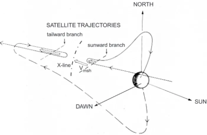
config-uration illustrated in Fig. 3, Bnis negative (pointing inward),
sunward of the X-line and positive (pointing outward), on the tailward side. A positive slope thus indicates a crossing sun-ward of the X-line, and a negative slope indicates a crossing on the tailward side. On the tailward branch of an X-line
SATELLITE TRAJECTORIES SUN NORTH DAWN tailward branch sunward branch X-line V msh
Fig. 3. A sketch that illustrates reconnection between a tailward
stretched magnetospheric field line in the Northern Hemisphere past dawn with an oppositely directed magnetosheath field line. The light arrows indicate plasma flow. The orientation of the X-line is shown by the dot-dashed line. Spacecraft crossings of the tail-ward and suntail-ward branches are schematically indicated. The ge-ometry shows the case with 180◦shear. For magnetosheath fields not anti-parallel to the magnetosphere field, the X-line is tilted more obliquely. Figure adapted from Gosling et al. (1986).
configuration, the magnetic curvature forces have the same sense as the magnetosheath flow and thus lead to enhanced flow speeds (plasma jetting). For a crossing on the sunward side the curvature forces have the opposite sense and thus no jetting would occur.
For an ideal RD, the magnitude of the slope of the regres-sion line should be equal to unity. But several effects can lead to lesser slopes. These include (1) stresses coming from the tangential component of ∇(p+Bz2/2µ0), where Bz is
the guide field during reconnection; (2) the anchoring of the guide field in slower-moving plasma on the two sides of a re-connection channel; (3) the presence of O+ions not resolved in the measurements, leading to incorrect Alfv´en velocities. As we will see later, there is strong evidence that slopes as low as 0.5 can be indicative of an RD.
The Wal´en tests were performed only for C1 and C3 cross-ings, for which reliable ion flow and density data from the CIS/HIA instruments are available. For some selected cases, Wal´en test results are reported in Sect. 5, while the overall statistics are reported in Sect. 6.3. It has been argued (Scud-der et al., 1999) that one should use electron bulk velocities for the Wal´en tests, because the magnetic field is tied to the electron fluid, and the ion bulk velocity will differ from the electron bulk velocity if electric currents are flowing. But as we will see later, this difference is small in the cases we have analyzed.
4.2 Boundary layer
Particle transfer across the magnetopause generates a bound-ary layer of magnetosheath-like plasma earthward of the magnetopause. If the magnetopause is locally a TD, then local plasma transfer can only be via some kind of
716 km SC1 SC2 SC3 SC4 0.1 1.0 10.0 Ne [1/cc] -40 -20 0 20 Bmax [nT] 10 20 30 40 50 |B| [nT] -200 -100 0 100 200 300 V, Vpar [km/s] 1 10 T ||, ⊥ [MK] 2356:00 2356:30 2357:00 2357:30 2358:00 2358:30 2359:00 0.0 0.5 1.0 1.5 Pressure [nPa] -11.1 -11.1 -14.5 -14.5 -3.1 -3.1 -11.1 -11.1 -14.5 -14.5 -3.1 -3.1 -11.1 -11.1 -14.5 -14.5 -3.1 -3.1 -11.1 -11.1 -14.5 -14.5 -3.1 -3.1 -11.1 -11.1 -14.5 -14.5 -3.2 -3.2 -11.1 -11.1 -14.5 -14.5 -3.2 -3.2 -11.1 -11.1 -14.5 -14.5 -3.2 -3.2 Xgse Ygse Zgse
Fig. 4. Plasma and magnetic field data for the outbound crossing
near 23:57 UT on 4 July 2001. From top to bottom, the panels are: plasma density (from EFW), maximum variance component and magnitude of the magnetic field (from FGM) for all four Clus-ter spacecraft, plotted as 6-s running averages with 0.2-s spacing; magnitude (diamonds) and parallel component (plus symbols) of the ion bulk velocities; parallel (plus symbols) and perpendicular (diamonds) ion temperatures; total pressure (plasma plus magnetic), all from CIS-HIA on spacecraft C1 and C3, plotted at spin resolu-tion (∼4 s). There is a data gap in the C3 plasma data right after the magnetopause transition. The magnetopause thickness from C1, calculated as described in Sect. 3.2, was 716 km for this case, and is shown as a horizontal bar in the Bmaxpanel. The time axis
ap-plies to the C1 measurements. The C2, C3, and C4 data have been shifted and stretched, in order to line up the crossings and turn them into spatial profiles, as described in the text. The position of C1 (in GSE coordinates) is given along the UT axis. Note the sharp rise in density at the inner edge of the magnetopause current layer.
sive process. As the plasma in the boundary layer tends to flow along the magnetopause at some fraction of the mag-netosheath speed, the locally observed boundary layer will reflect the accumulated entry occurring upstream from the observation site. Diffusion therefore creates a boundary layer with a thickness that increases with increasing distance from
801 km SC1 SC2 SC3 SC4 0.1 1.0 10.0 Ne [1/cc] 10 20 30 40 |B| [nT] 0 10 20 30 40 Bmax [nT] -200 -100 0 100 200 V, Vpar [km/s] 1 10 T ||, ⊥ [MK] 0021:00 0022:00 0023:00 0024:00 0025:00 0.0 0.5 1.0 1.5 Pressure [nPa] -3.5 -3.5 -11.5 -11.5 8.4 8.4 -3.5 -3.5 -11.5 -11.5 8.4 8.4 -3.5 -3.5 -11.5 -11.5 8.3 8.3 -3.5 -3.5 -11.5 -11.5 8.3 8.3 -3.5 -3.5 -11.5 -11.5 8.3 8.3 Xgse Ygse Zgse
Fig. 5. Plasma and magnetic field data for the inbound crossing near
00:22 UT on 5 July 2001, in the same format as Fig. 4. Note that C3 enters the hot plasma of the plasma sheet near 00:24 UT.
the subsolar point. If, on the other hand, the magnetopause is an RD, plasma enters the magnetosphere via fluid flow, at a speed, Vn, given by the Alfv´en velocity based on the
nor-mal magnetic field component, Bn. This inflow generates a
wedge-shaped boundary layer emanating from the reconnec-tion site (Levy et al., 1964). In this situareconnec-tion, the boundary layer thickness will increase with increasing distance from the reconnection site (the X-line). The identification of a boundary layer requires comparisons between the magnetic field and plasma density profiles measured across the mag-netopause.
5 Examples
In this section we discuss six magnetopause crossings in order to illustrate the range of characteristics of the magne-topause and boundary layer on this pass. For this discussion, the relative timing of the spacecraft crossings is unimportant,
and in Figs. 4–9 the traces from C2, C3 and C4 have there-fore been shifted and stretched (or compressed) relative to that of C1, so that the crossing times line up, and the four profiles represent spatial profiles, at least near the magne-topause, even though they are plotted against the C1 time.
The necessary time shift is simply a displacement of the C2, C3 and C4 curves based on the difference between their crossing times and that of C1. The time stretching of the C2, C3 and C4 curves is done in inverse proportion of their magnetopause speeds relative to that of C1. Thus, the plotted interval for each spacecraft is given by:
TSCn=TSC1∗
VMT V SC1
VMT V SCn
, n=2, 3, 4, (2)
where VMT V SCnis the magnetopause velocity according to
the MTV method (see Sect. 3.2) for spacecraft n, and TSCn
is the corresponding time interval shown. 5.1 23:57 UT crossing (#1)
This crossing is the first on this orbit and is labelled 1 in Fig. 1. The plasma and magnetic field data are shown in Fig. 4. Minimum variance analysis (MVAB) was performed on the C1 magnetic data and the resulting rotation matrix was then used to transform the magnetic field from all spacecraft into the same coordinate system. The magnetopause crossing is recognized as the transitions in the magnetic field magni-tude (from ∼45 nT to ∼20 nT) and in the maximum variance component (from ∼−45 nT to ∼20 nT). The total change in
Bmax corresponds to a rotation of almost 180◦ across the
magnetopause.
At the time the magnetic field begins its transition, i.e. at the inner edge of the magnetopause current layer, the plasma density increases abruptly from a magnetospheric level of a few tenths of cm−3to 10 cm−3. There is another increase by a factor of two near the outer edge of the magnetopause. Over the width of the magnetopause the plasma velocity increases to 250 km s−1. The ion temperature, which is not meaning-ful until shortly before the magnetopause crossing, when the density becomes measurable by HIA, shows a slight drop as expected for the exit from the magnetosphere. The total pres-sure (magnetic prespres-sure plus ion thermal prespres-sure) is reason-ably constant, as expected across the magnetopause. The fact that the plasma density shows no significant enhancement be-fore the magnetopause encounter means that on this cross-ing there was no magnetopause boundary layer, i.e. no layer of magnetosheath-like plasma located inward of the magne-topause. Using the MTV-method described in Sect. 3.2 on this set of crossings, we obtain magnetopause thicknesses of 716, 715, 706, and 680 km for C1 to C4, respectively. For reference, we have plotted the thickness for the C1 crossing as a horizontal bar in Fig. 4.
To determine whether the magnetopause was a TD or an RD, we performed a test of the Wal´en relation. As described in Sect. 4.1, this test compares the plasma flow velocity in the deHoffmann-Teller frame with the Alfv´en velocity. From the low values for the correlation coefficient and/or slope of the
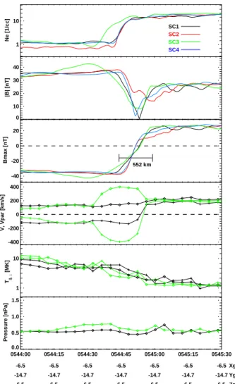
552 km SC1 SC2 SC3 SC4 1 10 Ne [1/cc] 0 10 20 30 40 |B| [nT] -40 -20 0 20 Bmax [nT] -400 -200 0 200 400 V, Vpar [km/s] 1 10 T ||, ⊥ [MK] 0544:00 0544:15 0544:30 0544:45 0545:00 0545:15 0545:30 0.0 0.5 1.0 1.5 Pressure [nPa] -6.5 -6.5 -14.7 -14.7 6.5 6.5 -6.5 -6.5 -14.7 -14.7 6.5 6.5 -6.5 -6.5 -14.7 -14.7 6.5 6.5 -6.5 -6.5 -14.7 -14.7 6.5 6.5 -6.5 -6.5 -14.7 -14.7 6.5 6.5 -6.5 -6.5 -14.7 -14.7 6.5 6.5 -6.5 -6.5 -14.7 -14.7 6.5 6.5 Xgse Ygse Zgse
Fig. 6. Plasma and magnetic field data for the outbound crossing
near 05:45 UT on 5 July 2001. Plot format and labelling as in Fig. 4. Note the pronounced plasma jetting observed by C3, directed in the
−B direction (V||<0) which is not observed by C1 (4th panel).
regression line found for this case, it is concluded that the magnetopause was a TD on this occasion. By definition, a TD does not permit local plasma entry by fluid flow. The fact that the observed plasma density stays at the low magne-tospheric values until the spacecraft enters the magnetopause current layer is consistent with such an impermeable bound-ary.
5.2 00:22 UT crossing (#2)
This inbound crossing, shown in Fig. 5, differs from the pre-vious example in that the magnetic field shear is small, only 30◦. The change in Bmax is correspondingly much smaller.
The positive sign of the shear indicates a northerly directed magnetosheath field. The magnetopause thickness obtained for the C1 crossing is ∼800 km. The present crossing is also distinguished by the presence of a boundary layer of mag-netosheath plasma inside the magnetopause, as evidenced by
187 km SC1 SC2 SC3 SC4 0.1 1.0 10.0 Ne [1/cc] -20 -10 0 10 20 Bmax [nT] 20 25 30 35 |B| [nT] -200 0 200 400 V, Vpar [km/s] 1 10 T ||, ⊥ [MK] 1058:30 1059:30 1100:30 1101:30 1102:30 1103:30 0.0 0.5 1.0 1.5 Pressure [nPa] -8.7 -8.7 -16.3 -16.3 4.0 4.0 -8.7 -8.7 -16.3 -16.3 4.0 4.0 -8.7 -8.7 -16.3 -16.3 4.0 4.0 -8.7 -8.7 -16.3 -16.3 4.0 4.0 -8.7 -8.7 -16.3 -16.3 4.0 4.0 -8.8 -8.8 -16.3 -16.3 4.0 4.0 Xgse Ygse Zgse
Fig. 7. Plasma and magnetic field data for the inbound
magne-topause crossing at 11:01 UT on 5 July 2001. Plot format and la-belling as in Fig. 4. Note the gradual density drop, the field-aligned plasma flow, and the large temperature anisotropy on the magne-topsheric side, which are the characteristics of the plasma mantle.
the lack of a sharp density drop at the inner edge of the mag-netopause. A closer look shows that the spacecraft have ac-tually entered the high latitude boundary layer known as the plasma mantle (Rosenbauer et al., 1975). Evidence for the plasma mantle are the alignment of the flow velocity with the magnetic field (as indicated by the near-equality of V and
V||), and the large temperature anisotropy, T⊥/T||.
This case also differs in another interesting aspect. While in the previous example the time-series measured by the four spacecraft were quite similar, the profiles of density, velocity and temperature recorded by C3 are now quite different from those of the other spacecraft. In one minute C3 has gone from the magnetosheath across the magnetopause into the hot plasma sheet (with T =∼6·107K), while the other three spacecraft are still in the magnetosheath. There is an indica-tion of a boundary layer in the C3 data, but its thickness must have been less than the spacecraft separation, otherwise the
other three spacecraft could not have remained in the mag-netosheath. (This time sequence is not apparent in Fig. 5 because in constructing the figure, the data were shifted so that the magnetopause crossings all line up.) When C1, C2, and C4 finally cross the magnetopause (∼90 s after C3), they enter the boundary layer, in the form of the cold plasma man-tle (with T =∼1·106K) and remain there, at nearly the same density levels, for several minutes. This is an indication that when those spacecraft entered the boundary layer, it must have been much thicker than the spacecraft separation. The explanation for this difference could either be temporal, im-plying a very rapid change in boundary layer thickness, or spatial, implying the existence of a boundary between dif-ferent plasma regimes: where C3 crossed, the plasma sheet abutted the magnetopause (almost) directly, while there was a thick plasma mantle where the other three spacecraft crossed. 5.3 05:45 UT crossing (#13)
This outbound crossing (with almost 180◦shear) has been
chosen to illustrate that the character of the magnetopause can change rapidly. Figure 6 shows that C3 observes plasma jetting when it enters the magnetopause, while C1, which crossed 25 s earlier, does not. (This relative timing is not apparent from the figure because it shows the inferred spatial profiles rather than the original time series, as described at the beginning of Sect. 5.)
The Wal´en test for C3 yields a slope of −0.76 (with cor-relation coefficient of −0.96). As described in Sect. 4.1, the negative slope means that the C3 crossing occurred tailward of an X-line, where the magnetic curvature forces lead to plasma jetting, as observed. The situation exists as shown by the tailward branch crossing in Fig. 3. The slope determined for C1 is only 0.19. Thus, the C1 crossing either occurred very near the X-line (where the Wal´en relation does not ap-ply), or at the time of the C1 crossing the magnetopause was a TD and changed to an RD over a short period of time. We believe that the latter case applies, because the C1-to-C3 sep-aration vector was nearly aligned with the magnetopause nor-mal at this time, and the C1 and C3 crossings must therefore have been close in space. Thus, it seems that between the times of the C1 and C3 crossings an X-line must have formed further upstream.
Comparing the density profiles (top panel of Fig. 6) with those of Bmax (second panel), it is evident that during the
C1, C2, and C4 crossings there was no boundary layer, while C3 observed a thin boundary layer. This is consistent with the conclusion that the magnetopause was a TD during the C1, C2, and C4 crossings, but had become an RD when C3 crossed it. Comparing the width of that boundary layer with the magnetopause width of ∼550 km (shown by the horizon-tal bar in the figure), the boundary layer thickness observed by C3 may be estimated at around 250 km. The fact that the boundary layer is so thin probably means that the C3 cross-ing occurred close to the X-line, where the wedge-shaped boundary layer is expected to be very narrow. If the X-line
was indeed close to the C3 crossing, then it becomes sig-nificant that the magnetosheath flow speed (at 205 km s−1) is substantially larger than the local Alfv´en speed (140 km s−1), which is not usually considered a likely condition for the formation of an X-line, unless the X-line is moving. We will return to this point in Sect. 6.
5.4 11:01 UT crossing (#20)
This inbound crossing with 65◦ magnetic shear (i.e. a northerly directed magnetosheath field), shown in Fig. 7, is characterized by three properties. First, the magnetopause is an RD. This conclusion is based on the slopes of the Wal´en relation, 0.60 and 0.72 for C1 and C3, respectively. Second, the positive sign of the Wal´en slopes implies that the crossing occurred sunward and southward of an X-line. Third, follow-ing the magnetopause crossfollow-ing the spacecraft are immersed in the most extended boundary layer of the entire day. Not-ing the smooth density profiles (top panel), the alignment of the plasma flow velocity with the magnetic field (indiated by the near-equality of V and V||, fourth panel), and the large
ion temperature anisotropy (fifth panel), one concludes that Cluster has actually encountered the plasma mantle. The magnetopause is rather thin at this time, around 190 km for the C1 crossing.
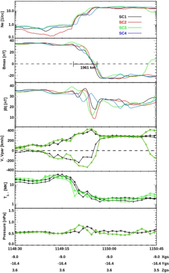
5.5 11:49 UT crossing (#21)
This high-shear (155◦) outbound pass, shown in Fig. 8, has been chosen for two reasons. First, it has a density drop near the center of the magnetopause current layer, followed by a density plateau until its inner edge. Such plateaus have been noted earlier in single-spacecraft data (Song et al., 1993). As this plateau is seen sequentially by all four spacecraft, it is a true spatial feature, and not the result of dwelling at a fixed location relative to the magnetopause, as could not have been excluded in single-spacecraft observations. The magnetopause thickness is 1960 km, and there is no bound-ary layer. Second, C1 and C3 show pronounced plasma jet-ting, indicating that the magnetopause is an RD and that the crossing occurred through the tailward branch. Thus, the ge-ometry for this case is as shown in Fig. 3 for crossings of the tailward branch, except that the magnetosheath field is not exactly opposite to the magnetosphere field in the present case. We obtain Wal´en slopes of −0.67 and −0.60, with cor-relation coefficients of −0.98 and −0.89, for C1 and C3, re-spectively. It should be noted, however, that the inner part of the magnetopause current layer had to be excluded from the test to obtain these high values. This implies that the plasma observed further inward has not entered locally.
5.6 15:26 UT crossing (#29)
This outbound crossing with −140◦shear (i.e. a tailward di-rected field with a southerly component) shown in Fig. 9, is considered an RD crossing through the tailward branch,
1961 km SC1 SC2 SC3 SC4 0.1 1.0 10.0 Ne [1/cc] -20 0 20 40 Bmax [nT] 10 20 30 40 |B| [nT] -400 -200 0 200 400 V, Vpar [km/s] 1 10 T ||, ⊥ [MK] 1148:30 1149:15 1150:00 1150:45 0.0 0.5 1.0 1.5 Pressure [nPa] -9.0 -9.0 -16.4 -16.4 3.6 3.6 -9.0 -9.0 -16.4 -16.4 3.6 3.6 -9.0 -9.0 -16.4 -16.4 3.6 3.6 -9.0 -9.0 -16.4 -16.4 3.5 3.5 Xgse Ygse Zgse
Fig. 8. Plasma and magnetic field data for the crossing near
11:49 UT on 5 July 2001. Plot format and labelling as in Fig. 4. Note the density plateau within the magnetopause, and the enhanced plasma flow speed observed by both C1 and C3.
as evident from the plasma jetting seen on C1 and C3. The Wal´en tests, however, yield slopes of only −0.60 and
−0.46 for C3 and C1, respectively. As already mentioned in Sect. 4.1, there are a number or reasons why RDs can have slopes less than one and this event supports this conclusion (see Sect. 6.3).
The magnetopause thickness obtained for the C1 crossing is ∼890 km. The plasma density stays at the magnetosheath level until the inner edge of the magnetopause, followed by an extended boundary layer with a density plateau at 2 cm−3, before dropping below 1 cm−3.
6 Statistical results
6.1 Magnetopause thickness, speed, and current
Applying the technique described in Sect. 3 to the 24 cross-ings by all four spacecraft, we obtain magnetopause thick-nesses, speeds and current densities for a total of 96
885 km SC1 SC2 SC3 SC4 0.1 1.0 10.0 Ne [1/cc] -10 0 10 20 30 Bmax [nT] 0 10 20 30 |B| [nT] -200 0 200 400 V, Vpar [km/s] 1 10 T||, ⊥ [MK] 1525:00 1525:30 1526:00 1526:30 1527:00 1527:30 1528:00 0.0 0.5 1.0 1.5 Pressure [nPa] -10.1 -10.1 -16.5 -16.5 1.6 1.6 -10.1 -10.1 -16.5 -16.5 1.6 1.6 -10.1 -10.1 -16.5 -16.5 1.6 1.6 -10.1 -10.1 -16.5 -16.5 1.6 1.6 -10.1 -10.1 -16.5 -16.5 1.6 1.6 -10.1 -10.1 -16.5 -16.5 1.6 1.6 -10.1 -10.1 -16.5 -16.5 1.6 1.6 Xgse Ygse Zgse
Fig. 9. Plasma and magnetic field data for the crossing at 15:26 UT
on 5 July 2001. Plot format and labelling as in Fig. 4. Note the density plateau on the magnetospheric side of the magnetopause.
ings. Figure 10 shows histograms of these quantities. Ta-ble 6.1 lists the individual thicknesses. They range from 100 to 2500 km, with a peak occurrence in the 400–800 km bin, and an average of 753 km. The speeds range from less than 10 km s−1up to 180 km s−1, with a peak in the 20–40 km s−1bin, and an average of 48 km s−1. These re-sults are quite similar to the earlier statistics from ISEE-1 and -2 dual spacecraft measurements (Berchem and Russell, 1982), although those were obtained for the dayside mag-netopause, covering local times between 08 and 17 h. Their average thickness was somewhat higher (923 km), but one should note that Berchem and Russell (1982) used the full 0–100% transition in Bmax to define the thickness, which
would make their values a bit higher. Similar average thicknesses (900 km) were also reported from AMPTE/IRM single-spacecraft analysis of dayside magnetopause cross-ings between 08 and 16 h local time (Phan and Paschmann, 1996).
Ion gyroradii and ion inertial lengths in the adjoining magnetosheath were typically 40–80 km for these crossings.
<100 <200 <400 <800 <1600 <3200 <6400 0 5 10 15 20 25 30 35 40 MP thickness [km] <5 <10 <20 <40 <80 <160 <320 0 5 10 15 20 25 30 35 MP speed [km/s] <0.01 <0.02 <0.04 <0.08 <0.16 <0.32 <0.64 0 5 10 15 20 25 30 35 40
Current density [uA/m ]2
‹d› = 753km ‹|v|› = 48 km/s ‹j› = 0.05 uA/m2 N u m be r o f e ve n ts N u m be r o f e ve n ts N u m be r o f e ve n ts
Fig. 10. Histograms of magnetopause (MP) speed, thickness and
current density for 24 dawn flank magnetopause crossings by all 4 spacecraft on 4/5 July 2001, resulting in a total of 96 individual crossings. Note that the bins are logarithmically spaced.
Scaling the magnetopause thicknesses by those characteris-tic lengths therefore does not alter the large thickness range we have observed. The plasma β in the adjoining magne-tosheath was in the range 0.5 to 2. Thus, our data do not allow one to check the significant reduction in average thick-ness reported for β>10 crossings by ISEE (Le and Russell, 1994) and AMPTE/IRM (Phan and Paschmann, 1996).
As shown in Fig. 10, current densities range from
<0.01 uA up to ∼0.3 uA, with an average value of 0.05 uA. The factor 30 between the highest and lowest value is the same as for the thickness range, and the current density roughly scales inversely with the thickness, thus preserving a nearly constant net current. As explained in Sect. 3.2, the curlometer technique will underestimate the current densities for the events in this study. Taking 15 cm−3for the typical magnetosheath plasma density on this pass, the average cur-rent density implies an average drift velocity between ions and electrons of ∼30 km s−1. This point will become impor-tant later.
Table 1. Magnetopause thicknesses for 96 crossings.
Time dC1[km] dC2[km] dC3[km] dC4[km] 23:57 716 715 706 680 00:22 802 728 766 778 00:30 234 235 234 234 00:44 657 749 688 652 02:06 177 177 177 177 02:11 316 268 314 278 02:40 855 1070 961 921 05:34 119 122 122 122 05:45 552 740 642 525 06:23 372 581 490 410 08:17 511 548 634 662 11:01 188 188 188 188 11:49 1961 1895 1674 1822 12:01 1483 1478 1350 1397 12:14 313 284 239 202 12:44 439 464 439 444 12:49 349 366 436 376 13:41 884 1052 1078 1045 14:06 443 459 459 455 15:11 538 575 514 561 15:26 886 911 1138 946 15:49 2148 2318 2265 2389 17:02 1049 908 1048 928 17:28 1537 1721 1264 1662 0 500 1000 1500 2000 2500 0.00 30.00 60.00 90.00 120.00 150.00 180.00 Thickness [km] S h e a r a n g le [ d e g ]
Fig. 11. Magnetic shear plotted versus magnetopause thickness for
the 96 crossings.
Early ISEE results by (Elphic and Russell, 1979) indicated a correlation between magnetopause current layer thickness and magnetic shear, although a later study (Berchem and Russell, 1982) did not confirm this result. Our results, shown in Fig. 11, do not suggest any clear shear dependence either. 6.2 Surface waves
To investigate if surface waves are responsible for at least some of the magnetopause crossings on this day, we have looked for systematic variations in magnetopause
-45° -90° -135° =0° XGSE -YGSE 45° Magnetosheath Magnetosphere out in Cluster trajectory 2 3 5 7 0 0 2 0 0 0 3 0 0 0 4 4 0 2 0 6 0 2 1 1 02 4 0 0 53 4 0 54 5 0 6 23 0 7 0 7 0 8 1 7 1 1 4 9 1 2 0 1 1 2 4 4 1 2 4 9 1 3 4 1 1 4 0 6 15 1 1 15 2 6 1 54 9 1 6 03 1 7 02 1 7 2 8 -100 -90 -80 -70 -60 -50 Event ID Inbound
Outbound In-out pair
Out-in pair
[°
]
Fig. 12. Top: Illustration of surface waves on the dawn flank
mag-netopause and definition of azimuth angle. The boundary normals of the inbound and outbound crossings should have different az-imuthal angles. Bottom: azimuth angle, θ , of the boundary normal for the 24 crossings, ordered chronologically from left to right along the abcissa. For most of the cases, there is a systematic difference in the normal direction for inbound (triangles) and outbound (dia-monds) crossings. The red arrows indicate crossing pairs with an orientation change as expected from surface waves.
orientation. From the four-spacecraft analysis we obtained the magnetopause orientation for the 24 crossings that in-volved all four spacecraft. Figure 12 shows the azimuthal angle, θ , of the magnetopause normals for these 24 cases. This angle is defined as θ = tan−1(n
x/ny). An azimuth angle
of 0◦thus means a normal pointing in the GSE +X direction, −90◦a normal vector pointing in the GSE -Y direction. The
figure shows that in cases where two subsequent crossings represent an in/out (or a out/in) pair, the inbound crossing has a larger azimuth angle than the outbound crossing, con-sistent with the passage of a surface wave, as illustrated in the top of Fig. 12.
Since the observed wave motion is not strictly periodic, it is difficult to draw any conclusions about the wavelengths. The time interval of the in-out pairs in Fig. 12 varies from 5 min up to 26 min, but these times may contain several wave periods. For reference, a 5 min period corresponds to a wave length of around 7 RE, assuming that the waves propagate at half the observed magnetosheath flow speed.
For magnetopause traversals induced by surface waves, one can distinguish crossings of the leading and trailing edges of the waves. To investigate whether there are system-atic differences in thicknesses and/or speed between the lead-ing and traillead-ing edges, we have separated the crosslead-ings into leading edge (i.e. inbound) crossings, and trailing edge (i.e. outbound) crossings. We found that the inbound crossings
>1 >0.9 >0.8 >0.7 >0.6 >0.5 >0.4 >0.3 >0.2 >0.1 >0.0 0 2 4 6 8 Walenslope N um be r of e ve nt s <=30 <=60 <=90 <=120 <=150 <=180 0 2 4 6 8 Positive Negative
Shear angle [deg]
N um be rs o f e ve nt s Positive Negative >1 >0.9 >0.8 >0.7 >0.6 >0.5 >0.4 >0.3 >0.2 >0.1 >0.0 0 2 4 6 Walenslope N um be r of e ve nt s <=30 <=60 <=90 <=120 <=150 <=180 0 2 4 6 8 Positive Negative
Shear angle [deg]
N um be rs o f e ve nt s Positive Negative
Fig. 13. Top: Histogram of Wal´en slopes, for all cases where the
correlation coefficient magnitude exceeded 0.85. Positive and neg-ative slopes are shown with different colors. Bottom: Subset of cases with slopes of magnitude >0.5, divided according to the sign of the slopes, versus the magntitude of the magnetic shear across the magnetopause.
have an average thickness of 613 km, while the outbound crossings have an average thickness of 861 km. This differ-ence is, however, not statistically significant. There is also no significant speed difference.
6.3 RD vs. TD statistics
In Sect. 5 we already reported the results of the Wal´en test, described in Sect. 4.1, for a number of crossings. In this sec-tion we will present the overall statistics. In addisec-tion to the 24 crossings by all four spacecraft, there were several well-defined crossings in which fewer than four were involved. With those additions, we had a total of 60 crossings available for the statistical analysis, 31 from C1 and 29 from C3.
Of these 60 cases, 36 gave correlation coefficients
|cc|>0.85 between (V−VHT) and VA, 16 for C1 and 20 for
C3. Figure 13 (top) shows a histogram of the slopes of these 36 cases. The magnitude and sign of the Wal´en slope vary rapidly from crossing to crossing, but the C1 and C3 results (not separated in the figure) are closely matched in magni-tude and sign. In fact, of the 13 crossings where we have obtained results (with |cc|>0.85) for both spacecraft, 11 had very similar slopes. This result lends credence to the reliabil-ity of the method. We note here that the use of ion bulk veloc-ities for the Wal´en test does not introduce significant errors,
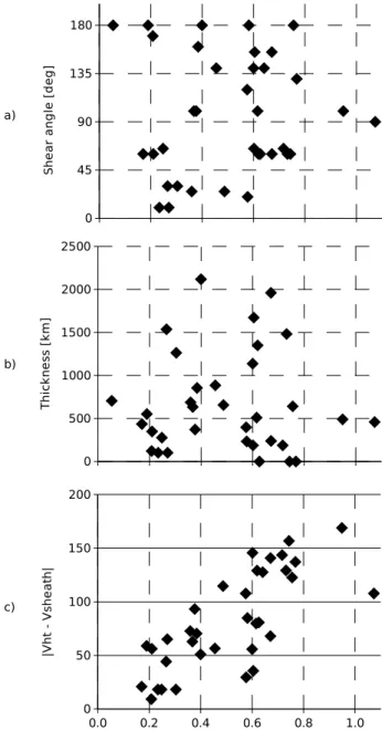
0.0 0.2 0.4 0.6 0.8 1.0 0 45 90 135 180 S h e a r a n g le [ d e g ] 0.0 0.2 0.4 0.6 0.8 1.0 0 500 1000 1500 2000 2500 T h ic k n e ss [ k m ] 0.0 0.2 0.4 0.6 0.8 1.0 0 50 100 150 200 |V h t V sh e a th | a) b) c)
Fig. 14. Magnitude of the magnetic shear (a), magnetopause
thick-ness (b), and magnitude of the velocity residue (Vmsh−VH T) (c), plotted versus the magnitude of the Wal´en relation slope, for all cases where the correlation coefficient magnitude exceeds 0.85. While there is no correlation of the Wal´en slope with either mag-netic shear or magnetopause thickness, there is a clear correlation with the difference between magnetosheath and deHoffmann-Teller velocities, indicating that magnetic coupling increases with increas-ing Wal´en slope.
and thus cannot explain the deviations from unity because, as shown in Sect. 6.1, typical ion-electron velocity differences were only 30 km s−1.
As already discussed in Sect. 4.1, RDs should ideally re-sult in slopes with magnitude 1, but other effects could cause deviations from 1. Perfect agreement between the observed plasma flows and those predicted for an RD is rare. In most cases reported in the literature the observed flows are smaller
than predicted (e.g., Sonnerup et al., 1981; Gosling et al., 1986; Paschmann et al., 1986; Phan et al., 1996). The well-pronounced plasma jets in Fig. 8 had slopes of −0.67 (C1) and −0.60 (C3). Similarly, the jets in Fig. 9 have slopes of
−0.46 (C1) and −0.60 (C3). As no alternate explanation for such plasma jetting appears to exist, we feel justified to clas-sify cases with slopes in excess of 0.5 as RDs.
Using 0.5 as the threshold for the slope, 19 of the 60 cross-ings were RDs, 8 by C1 and 11 by C3. As mentioned earlier, the sign of the Wal´en slope indicates whether a crossing oc-curred sunward or tailward of the reconnection site. Of the 19 RD crossings, 12 had positive Wal´en slopes, i.e. were sun-ward crossings, and 7 had negative slopes, i.e. were tailsun-ward crossings. Plotting the occurrence of positive and negative slopes versus the magnitude of the magnetic shear across the magnetopause (Fig. 13, bottom), one notices a strong asym-metry: cases with large shear have predominantly negative slopes, i.e. they occur tailward of the reconnection site, while lower shear crossings occur predominantly on the sunward side.
On the other hand, the magnitude of the Wal´en slopes is not correlated with magnetic shear, as demonstrated in Fig. 14a. The figure also shows that slopes >0.5 occur for shear angles ≥60◦, except for one case where the shear is
only 20◦. To test whether the magnetopause thickness
de-pends on its characterization as RD or TD, Fig. 14b plots the magnetopause thickness versus the Wal´en slope magnitude. No dependence is apparent.
If the magnetopause is a TD, then there is no magnetic coupling across the magnetopause, and the HT frame should be well-anchored in the magnetosheath plasma, i.e. the dif-ference between the magnetosheath velocity and the HT ve-locity should be small (e.g., Hasegawa et al., 2004b). If it is an RD, the opposite should hold, i.e. the difference between the magnetosheath velocity and the HT velocity should be large. In Fig. 14c we have plotted the magnitude of the dif-ference, |Vmsh−VH T|, between the magnetosheath and HT
velocities versus the Wal´en slope. The figure shows that there is a clear trend, in the sense that the velocity difference be-comes larger for larger slopes, confirming the effect of mag-netic coupling.
6.4 Boundary layer statistics
For all 60 crossings by C1 and C3 we have determined whether a boundary layer was observed, by comparing the 0.2-s resolution magnetic field and plasma density profiles. We found that 25 of the 60 crossings (i.e. 42%) showed no sign of a boundary layer at the location of the crossing. Good examples are the crossings at 23:57 (Fig. 4), at 05:45 (Fig. 6), except for the C3 crossing, and 11:49 (Fig. 8). In our statis-tics, crossings without a trace of a boundary layer are referred to as Category 1.
The remaining 35 cases showed boundary layers of vary-ing character or extent. When a thin boundary layer exists, one can estimate its thickness using the speed determined from the adjacent magnetopause crossing. An example is the
05:45 crossing by C3. But for boundary layers with longer durations and/or irregular (e.g., non-monotonic) density pro-files, a thickness definition and determination is difficult. To avoid this problem we have sorted all boundary layers into just three more categories. Category 2 are the cases with thin boundary layers. Category 3 comprises cases with a more extended boundary layer, with an initial sharp density drop at the magnetopause, followed by a medium-density (a few cm−3) boundary layer, often appearing as a density plateau. An example is the 15:26 crossing (Fig. 9). Finally, category 4 is for extended boundary layers without much drop at the magnetopause. The 11:00 UT crossing (Fig. 7) is such an example. In all Category 4 cases the boundary layer was ac-tually the plasma mantle itself. Figure 15 shows the number of crossings versus the boundary layer category as just de-fined.
An interesting subset of the crossings without a boundary layer are those that were classified as RDs in the previous section. There are eight such cases. Because of the wedge-shape of the boundary layer resulting from reconnection, RDs should have a thickness near zero only when crossed close to the X-line, as already discussed in Sect. 5.3. But if this interpretation is correct, it follows that the observed local magnetic shear should also be representative of the magnetic shear at the X itself. Of the eight crossings in this category only three have large shear angles (≥140◦). One case has a shear angle of 120◦, and the remaining four have values
≤100◦. In those cases the reconnecting fields are far from being anti-parallel.
If these eight crossings are indeed close to the X-line, then it also follows that the Alfv´en Mach number, MA, in the
ad-joining magnetosheath should be representative of the MAat
the X-line itself. It is thus highly significant that in all cases
MA>1, with values ranging from 1.2 to 2.1. Of the 8 cases,
two occurred on the tailward branch, and the other 6 on the sunward branch.
7 Summary and conclusion
We have analyzed all well-defined magnetopause crossings on a single Cluster orbit that skimmed the near-tail dawnside magnetopause at GSM local times between 5.0 and 3.8 h and GSM latitudes between 32◦and 4◦. By including all cross-ings in a long sequence, subjective selections were avoided. The crossings are characterized by a stable magnetic field orientation on the magnetosphere side, but quite variable field directions on the magnetosheath side, giving rise to magnetic shear angles that ranged between ∼0◦and ∼180◦. A magnetic signature was observed in all these crossings, usually both a field rotation and a change in field strength. The magnetopauses were well-resolved in the data. Even the shortest crossing included more than 20 magnetic field samples (at 0.2 s spacing). We obtained magnetopause ori-entation, speed, thickness, and currents from four-spacecraft analysis of 24 complete passes, i.e. for a total of 96 individ-ual magnetopause crossings. There were other crossings that
Type 1 Type 2 Type 3 Type 4
0 5 10 15 20 25
30 Boundary Layer Category
N u m b e r o f e v e n ts
Fig. 15. Histogram of boundary layer classifications for the C1 and
C3 crossings. There are 25, 18, 11, and 6 crossings of types 1 (no boundary layer) to 4 (extended high density boundary layer), re-spectively.
involved fewer than four spacecraft, which were included in the single-spacecraft analysis of the TD/RD and boundary layer classifications. A total of 60 C1 and C3 crossings were analyzed this way.
The main results may be summarized as follows:
Magnetopause thickness. Magnetopause current sheet thicknesses on this pass range from 100 to 2500 km, but with the majority of the events having a thickness in the 400 to 800 km range, with an average of ∼750 km. As al-ready noted, these results are in agreement with the ISEE and AMPTE/IRM results (Berchem and Russell, 1982; Phan and Paschmann, 1996), although those were obtained for loca-tions sunward of the dawn-dusk terminator, with local times ranging between 08 and 17 h, while ours were taken at loca-tions past the terminator, at local time times between 3.8 and 5.0 h. The fact that the magnetopause thickness does not ap-pear to systematically grow with distance from the subsolar point implies that the diffusion coefficient for the current is low.
Normalization to either to the magnetosheath ion gyrora-dius or ion inertial length did not alter this large dynamic range, because those characteristic lengths were fairly stant themselves, of the order of 50 km. So one must con-clude that the magnetopause thickness is not controlled by those characteristic scales. There also appears to be no cor-relation between magnetopause thickness and local magnetic shear angle, confirming the result of Berchem and Russell (1982). The thickness reduction for large (>10) plasma-β reported in the literature (Le and Russell, 1994; Phan and Paschmann, 1996) could not be checked because β was <2 in our cases.
Note that the spacecraft separation distances impose some constraints for the multi-spacecraft methods. In order to tra-verse all four spacecraft, the amplitude of magnetopause mo-tion needs to be larger than the spacecraft separamo-tion dis-tances, i.e. ∼3000 km on this pass. Our results unavoidably contain this bias.
20 to 80 km s−1, with extremal velocities up to 180 km s−1. The average velocity is 48 km s−1. This result is also in good agreement with the ISEE and AMPTE/IRM results.
Magnetopause orientation. Magnetopause orientations in
general were consistent with expectations from a model mag-netopause, but close pairs of inbound/outbound crossings showed systematic variations in tilt angles, indicative of the passage of surface waves.
Current density. Current densities range from <0.01 to ∼0.30 µA m−2, with an average of 0.05 uA. For those cross-ings with large shear, i.e. those with similarly large 1Bmax,
the current densities were inversely proportional to magne-topause thickness, so that the total current was about the same, as required when the field change across the magne-topause remains constant.
Rotational versus tangential discontinuities. Based on
tests of the Wal´en relation, 19 of the 60 C1 and C3 crossings could be classified as RDs, if one adopts a slope in excess of 0.5 as the RD criterion. The observation of plasma jet-ting lends credence to the identification of cases with Wal´en slopes of only 0.5 as RDs. The tendency for the difference between magnetosheath and HT velocities to increase with increasing Wal´en slope supports the notion that large Wal´en slopes are indicative of strong magnetic coupling across the magnetopause.
Of the 19 cases identified as RDs, 12 had postive Wal´en slopes and 7 had negative Wal´en slopes. There is an inter-esting asymmetry in the distribution of the cases with pos-itive and negative Wal´en slope as a function of shear. The cases with large shear had predominantly negative slopes (i.e. were crossings tailward of the reconnection site, while lower shear cases all had positive slopes, i.e. were crossings sun-ward (and southsun-ward or northsun-ward, depending on the sign of the shear angle) of the reconnection site.
In none of the cases have we observed the actual passage of an X-line, i.e. a sign switch of the Wal´en slope in be-tween spacecraft crossings. If all reconnection sites were created on the dayside magnetopause and stayed there, then only negative slopes should have been observed. The cases with a positive slope could mean (a) that the X-line, although having been formed further sunward, had moved past the spacecraft location by the time those crossings occurred; or (b) that those X-lines were already located tailward of Clus-ter when they were formed. It is the flow speed relative to the Alfv´en speed in the magnetosheath at the reconnection site that should determine whether the X-line is stationary or moves (e.g., La Belle-Hamer et al., 1995). But without knowledge of the conditions at the X-line one cannot tell. As we will argue below, the subset of RDs without a boundary layer can provide this knowledge.
Boundary Layer. Our analysis has found that 26 of the 60
individual C1 and C3 crossings show no trace of a boundary layer, thus confirming earlier ISEE results (Sckopke et al., 1981) that the dawn flank LLBL thickness is highly variable. Our results do not confirm the conclusion of Mitchell et al. (1987), based on ISEE data as well, that the LLBL becomes thicker with increasing distance from the subsolar point. The
only crossings we observed having a substantial boundary layer are actually not crossings into the LLBL, but into the plasma mantle. Of the 26 crossings without boundary layer, 8 were identified as RDs.
Magnetopause crossings without a boundary layer have been reported earlier. Papamastorakis et al. (1984) discussed a low-latitude dayside crossing by ISEE-1 and -2 with large magnetic shear that showed no sign of an LLBL, in spite of adequate time resolution of the data. That crossing was iden-tified as a TD, based on the failure to satisfy the jump condi-tions for an RD. Gosling et al. (1986) have analyzed ISEE crossings of the near-tail dusk magnetopause and found a large number of accelerated flow events, i.e. crossings tail-ward of an X-line, without evidence for a boundary layer. Their crossings were characterized by almost antiparallel fields (nearly 180◦ shear). The evidence for crossings on
the sunward side of the X was not so clear. Interestingly, Gosling et al. (1986) report that accelerated flow events are much rarer among the ISEE crossings of the near-tail dawn magnetopause, where our measurements were made. They speculated that this asymmetry might be explained in terms of a combined latitude-seasonal effect in the ISEE sampling of the near-tail dusk and dawn magnetopause.
From a statistical analysis of ISEE-2 and AMPTE/CCE data, Eastman et al. (1996) concluded that nearly 10% of the crossings, which included the dawn and dusk flanks, ex-hibited no trace of a boundary layer. Eastman et al. sug-gested that the lack of a boundary layer indicated that these were crossings close to an X-line, although they did not ac-tually know whether the crossings were RDs. The eight RD cases without a boundary layer that we have found would fit this picture. But if these indeed are crossings close to an X-line, then one should expect the observed magnetic shear and Alfv´en Mach number to be representative of the condi-tions at the X-line itself. It is therefore interesting that four of the eight cases had shear angles ≤100◦, i.e. the magnetic fields were far from being anti-parallel. If the interpreta-tion of these cases as crossings close to the X-line is cor-rect, their magnetic shear would thus be inconsistent with the anti-parallel reconnection hypothesis. Furthermore, all eight cases had Alfv´en Mach numbers MA>1 in the
adjoin-ing magnetosheath, a situation where, accordadjoin-ing to conven-tional wisdom, the reconnection site (the X-line) cannot sit still. So if those crossings did indeed occur close to an X-line, the X-line was probably moving tailward rapidly.
A final point concerns the crossings without a bound-ary layer that are not RDs but TDs. To observe TDs with no boundary layer at such large distances from the subso-lar point appears to rule out diffusion over subso-large portions of the magnetopause as an effective means for plasma transport across the magnetopause.
Appendix A
In this appendix, a brief summary is presented of previ-ously existing multi-spacecraft methods for determination of
magnetopause orientation, motion, and thickness. Also, the new method (MTV) applied in this paper is described in de-tail.
Assume that the instantaneous magnetopause velocity is expressed by:
V (t )=A0+A1t + A2t2+A3t3, (A1)
where A0, A1, A2, andA3 are constants to be determined from the crossing times and durations. With the above ex-pression for V(t), we find the magnetopause thicknesses, di
(i=0,1,2,3), to be di = Z ti+τi ti−τi V (t )dt =2τi h V (ti) + (A2τi2)/3 + A3tiτi2 i . (A2)
The center crossing times, ti, where t3>t2>t1>t0, and cor-responding crossing durations, τi, are considered as known
quantities. The distance travelled by the magnetopause, be-tween crossing CRi and crossing CR0 (not to be confused
with the Cluster spacecraft naming convention; C1. . .C4) along a fixed normal direction, n, is then
Ri·n = Z t =ti t =0 V (t )dt =A0ti+ A1ti2 2 + A2ti3 3 + A3ti4 4 (A3)
where CRi is relative to that producing CR0.
In the Constant Velocity Approach (CVA), the coefficients
A1, A2, and A3are put to zero so that A0becomes the con-stant, but unknown velocity. The three Eqs. (A3) can then be solved for the vector m=n/A0, and A0can be obtained from the normalization |n|2=1.
In the Constant Thickness Approach (CTA), the thick-nesses di are assumed the same, di=d for i=0,1,2,3. The
four Eqs. (A2) can then be solved for the four quantities
A0/d, A1/d, A2/d and A3/d and, subsequently, the three Eqs. (A3) for the vector m=n/d. Finally, the thickness d is obtained from the normalization of n.
In the Discontinuity Analyzer (DA) approach, the normal direction is taken from some single-spacecraft method, such as minimum variance analysis of the magnetic field (MVAB) or minimum Faraday residue (MFR) analysis (Khrabrov and Sonnerup, 1998). Equations (A3) can then be solved for the coefficients A0, A1, and A2but A3must be put to zero. The DA approach is not a pure multi-spacecraft timing method because it makes use of a normal vector obtained from single-spacecraft data analysis. It has the advantage that it permits both velocity and thickness of the magnetopause to vary from crossing to crossing in an event. Its disadvantage is that the velocity polynomial in equation (A1) becomes quadratic rather than cubic, which is less flexible and can more easily lead to unreasonable results. Detailed illustra-tions of CVA, CTA, and DA (in the version decribed here),
have been given by Haaland et al. (2004) for one of the 5 July 2001, magnetopause crossings (at 06:23 UT).
The new MTV method is a combination of CVA, CTA, and DA, but uses no single-spacecraft methods and produces a cubic velocity polynomial. In the MTV method, the normal vector is obtained as a combination of the two normal vec-tors obtained from CVA and CTA, which are usually not the same (if they are the same, then the crossing has both con-stant velocity and concon-stant thickness). In the body of this pa-per the combination of the two normal vectors is taken to be their renormalized average but there may be circumstances where it is justified to place more emphasis on one normal than on the other. Once the combined normal is known, the MTV method uses DA, i.e. Eq. (A3), to provide three of the four equations needed to determine the velocity coefficients
A...A3. Rather than putting A3=0, a fourth equation is
ob-tained from the subsidiary condition that the variance of the thicknesses seen at the four spacecraft should be a minimum. This condition is again not unique. It is motivated by the ar-gument that the thickness variations are expected to be much smaller than the velocity variations during a typical event. The algebraic details of the MTV method are as follows:
The average thickness seen by the four spacecraft is
hdi=1 4 i=3 X i=0 di, (A4)
where the expressions for diare given by Eq. (A3). The
vari-ance in thickness can be written as
σ2=1 4 i=3 X i=0 [di− hdi]2= hdi2i − hdii2, (A5)
which is a quadratic form in the coefficients A0. . .A3. The minimization of this form with respect to A0, say, is written as
d dA0
σ2=0. (A6)
In performing the differentiation, one must remember that the four velocity coefficients A0. . .A3are interrelated via the three Eqs. (A3). The derivatives dA1/dA0, dA2/dA0, and
dA3/dA0 can be obtained by differentiation of those three equations. When the expressions for these derivatives are substituted into Eq. (A6), one obtains, after considerable al-gebra, the following linear relationship
K0A0+K1A1+K2A2+K3A3=0, (A7)
which can be used together with the three equations (A3) to provide four linear equations for the four velocity coefficients
A0. . .A3. The constants K0. . .K3in Eq. (A7) are given by
K0= 1hT τ i hT i K1= 1hT τ t i hT i