HAL Id: tel-01412590
https://pastel.archives-ouvertes.fr/tel-01412590
Submitted on 8 Dec 2016
HAL is a multi-disciplinary open access
archive for the deposit and dissemination of
sci-entific research documents, whether they are
pub-lished or not. The documents may come from
teaching and research institutions in France or
abroad, or from public or private research centers.
L’archive ouverte pluridisciplinaire HAL, est
destinée au dépôt et à la diffusion de documents
scientifiques de niveau recherche, publiés ou non,
émanant des établissements d’enseignement et de
recherche français ou étrangers, des laboratoires
publics ou privés.
Crowd dynamics : modeling pedestrian movement and
associated generated forces
Bachar Kabalan
To cite this version:
Bachar Kabalan. Crowd dynamics : modeling pedestrian movement and associated generated forces.
Structures. Université Paris-Est, 2016. English. �NNT : 2016PESC1126�. �tel-01412590�
L’UNIVERSIT´
E PARIS-EST
Sp´
ecialit´
e : Structures et Mat´
eriaux
par
Bachar KABALAN
Sujet de la th´
ese :
Dynamique des foules :
mod´
elisation du mouvement des pi´
etons et forces
associ´
ees engendr´
ees
Soutenue le 12 Janvier 2016 devant le jury compos´
e de :
Rapporteurs
Abdelilah HAKIM
Universit´
e Cadi Ayyad
Jean-Mathieu MENCIK
Institut National des Sciences Appliqu´
ees
Centre Val de Loire
Examinateurs
Patrice AKNIN
SNCF
Gwendal CUMUNEL
Ecole des Ponts ParisTech
´
Stefano DAL PONT
Universit´
e Joseph Fourier
Silvano ERLICHER
EGIS Industries
Fabien LEURENT
Laboratoire Ville Mobilit´
e Transport
Invit´
e
Bruno SOULIER
ENS de Cachan
very much enjoyed all the scientific discussions we had together not to mention the jokes and the laughs we shared.
I would also like to thank my supervisor, Gwendal Cumunel, for all the help that he gave me in order to finish my work rapidly and efficiently. I am grateful for his patience in helping me find the errors in my work and correcting them.
I would also like to extend my appreciation to the president of my thesis committee Professor Fabien Leurent and the reviewers who accepted to evaluate my thesis Professor Abdelilah Hakim and Jean-Mathieu Mencik.
I would like to show my gratitude to all my colleagues especially those with whom I have shared the office and who became dear friends. My deepest appreciation to all the friends I made in France during the past three years. I would particularly like to thank two of my closest friends Hassan Shukor and Mohammad Rammal for being there for me whenever I needed.
My deepest heartfelt appreciation goes to my family. Amal, Mahmoud and Leila all lived abroad and where examples for me on how to deal with the hardships of being away from home. To my parents Afaf and Ali to whom I owe everything I am grateful for. They have been the major motive for me to pursue this path and finish it successfully. It would take me several lifetimes to thank them for what they have done for me and my siblings.
Knowledge is better than wealth. Knowledge guards you while you have to guard wealth. Wealth decreases by spending while
knowledge increases by spending, and the results of wealth die as wealth decay. With knowledge a man acquires obedience during his lifetime and a good name after his death. Knowledge is a ruler while wealth is ruled upon.
Ali ibn Abi Taleb
The noblest pleasure is the joy of understanding.
mettent aux chercheurs de plusieurs disciplines, comme les sciences sociales ou la biom´ecanique, de mieux ´etudier et comprendre les mouvements des pi´etons et leurs interactions. Quant aux sciences de la s´ecurit´e et du transport, ils y voient des applications concr`etes comme le d´eveloppement de mod`eles de foule capables de simuler l’´evacuation d’un lieu public de moyenne ou de forte affluence, afin que les futures constructions ou am´enagements publics puissent offrir une qualit´e de s´ecurit´e et de service optimale pour les usagers.
Dans le cadre de cette th`ese, nous avons travaill´e sur le perfectionnement du mod`ele discret propos´e et d´evelopp´e par l’´equipe dynamique du laboratoire Navier. Dans ce mod`ele, les actions et les d´ecisions de chaque pi´eton sont trait´ees individuellement. Trois aspects du mod`ele ont ´et´e trait´es dans cette th`ese. Le premier concerne la navigation des pi´etons vers leurs destinations. Dans notre mod`ele, un pi´eton est repr´esent´e par une particule ayant une direction et une allure souhait´ees. Cette direction est obtenue par la r´esolution d’une ´equation eikonale. La solution de cette ´equation permet d’obtenir un champ de vitesses qui attribue `a chaque pi´eton, en fonction de sa position, une direction vers sa destination. La r´esolution de l’´equation une fois ou `a une p´eriode quelconque donne la strat´egie du chemin le plus court ou le plus rapide respectivement. Les effets des deux strat´egies sur la dynamique collective de la foule sont compar´ees.
Le deuxi`eme consiste `a g´erer le comportement des pi´etons. Apr`es avoir choisi son chemin, un pi´eton doit interagir avec l’environnement (obstacles, topologie, ...) et les autres pi´etons. Nous avons r´eussi `a int´egrer trois types de comportement dans notre mod`ele: (i) la pouss´ee en utilisant une approche originale, bas´ee sur la th´eorie des collisions des corps rigides dans un cadre thermodynamique rigoureux, (ii) le passage agressif (forcer son chemin) mod´elis´e par une force sociale r´epulsive et (iii) l’´evitement “normal” en adoptant une approche cognitive bas´ee sur deux heuristiques. Les performances des trois m´ethodes ont ´et´e compar´ees pour plusieurs crit`eres.
Le dernier aspect concerne la validation et la v´erification du mod`ele. Nous avons r´ealis´e une ´etude de sensibilit´e et valid´e le mod`ele qualitativement et quantitativement. `A l’aide d’un plan d’exp´erience num´erique nous avons r´eussi `a identifier les param`etres d’entr´ee ayant les effets principaux sur les r´esultats du mod`ele. De plus, nous avons trouv´e les diff´erentes interactions entre ces param`etres. En ce qui con-cerne la validation qualitative, nous avons r´eussi `a reproduire plusieurs ph´enom`enes d’auto-organisation. Enfin, nous avons test´e la capacit´e de notre mod`ele `a reproduire des r´esultats exp´erimentaux issus de la litt´erature. Nous avons choisi le cas du goulot d’´etranglement. Les r´esultats du mod`ele et ceux de l’exp´erience ont ´et´e compar´es.
Ce mod`ele de foule a ´egalement ´et´e appliqu´e `a l’acheminement des pi´etons dans la gare de Noisy-Champs. L’objectif de cette application est d’estimer le temps de stationnement des trains dans la gare.
Mots cl´es: Mouvement de foule, strat´egie de d´eplacement, navigation, interactions pi´eton-pi´eton,
val-idation et v´erification, ph´enom`enes d’auto-organisation.
bio-mechanics, who are interested in studying crowd movement and pedestrian interactions were able to better examine and understand the dynamics of the crowd. Professionals from architects and transport planners to fire engineers and security advisors are also interested in crowd models that would help them to optimize the design and operation of a facility.
In this thesis, we have worked on the imporvement of a discrete crowd model developed by the researchers from the dynamics group in Navier laboratory. In this model, the actions and decisions taken by each individual are treated. In its previous version, the model was used to simulate urgent evacuations. Three main aspects of the model were addressed in this thesis.
The first one concerns pedestrian navigation towards a final destination. In our model, a pedestrian is represented by a disk having a willingness to head to a certain destination with a desired direction and a desired speed. A desired direction is attributed to each pedestrian, depending on his position from the exit, from a floor field that is obtained by solving the eikonal equation. Solving this equation a single time at the beginning of the simulation or several times at during the simulation allows us to obtain the shortest path or the fastest path strategy respectively. The influence of the two strategies on the collective dynamics of the crowds is compared.
The second one consists of managing pedestrian-pedestrian interactions. After having chosen his/her direction according to one of the available strategies, a pedestrian is bound to interact with other pedestri-ans present on the chosen path. We have integrated three pedestrian behaviors in our model: (i) pushing by using an original approach based on the theory of rigid body collisions in a rigorous thermodynamics context, (ii) forcing one’s way by introducing a social repulsive force and (iii) “normal” avoidance by using a cognitive approach based on two heuristics. The three methods are compared for different criteria.
The last aspect is the validation and verification of the model. We have performed a sensibility study and validated the model qualitatively and quantitatively. Using a numerical experimental plan, we identified the input parameters that are the most statistically significant and estimated the effects of their interactions. Concerning qualitative validation, we showed that our model is able to reproduce several self-organization phenomena such as lane formation. Finally, our model was validated quantitatively for the case of a bottleneck. The experimental results are very close to the ones obtained from simulations. The model was also applied to pedestrian movement in the Noisy-Champs train station. The objective of the study was to estimate the train dwell time. The simulation results were similar to the observations.
Keywords : Crowd movement, displacement strategies, navigation, pedestrian-pedestrian interactions,
validation and verification, self-organization phenomena.
List of tables 24
Notations 25
1 Introduction 27
1.1 Crowd Management-History . . . 28
1.2 What is a crowd? . . . 29
1.3 Why simulate crowd motion and evacuation processes? . . . 30
2 Resum´e ´etendu 35 2.1 Introduction. . . 36
2.2 Etude bibliographique . . . 36
2.2.1 Etat de l’art des mod`eles de mouvement de foule . . . 36
2.2.2 Mod`eles de dynamique des fluides ou des gaz . . . 37
2.2.3 Mod`eles d’automates cellulaires . . . 37
2.2.4 Mod`eles de forces sociales . . . 38
2.3 Mod`ele discret . . . 38
2.3.1 Loi de comportement . . . 40
2.3.2 Volont´e de d´eplacement d’un pi´eton . . . 41
2.4 Strat´egies de d´eplacement . . . 43
2.4.1 M´ethode d’obtention du champ de vitesses souhait´ees . . . 43
2.4.2 Champ statique de vitesses . . . 44
2.4.3 Champ dynamique de vitesses. . . 44
2.5 Interactions pi´eton-pi´eton . . . 46
2.5.1 Force de r´epulsion sociale . . . 46
2.5.2 Approche cognitive. . . 47
2.5.3 Expression de h(α) . . . 47
2.5.4 Simulations num´eriques . . . 50
2.6 Validation et verification du mod`ele . . . 52
2.6.1 Validation quantitative: cas du goulot d’´etranglement . . . 52
2.6.2 Plans d’exp´eriences num´erique . . . 54
2.6.3 Estimation des effets principaux et leurs interactions . . . 55
2.6.4 Analyse de variance: quels sont les effets principaux?. . . 56
2.6.5 Mod`eles de regression . . . 58
2.7 Cheminement des pi´etons en gare . . . 60
2.7.1 G´eom´etrie de la gare de Noisy-Champs . . . 61
2.7.2 Trafic des trains . . . 62
12 CONTENTS
2.7.3 Trafic des voyageurs . . . 63
2.7.4 R´esultats . . . 64
2.8 Mod´elisation de la force lat´erale engendr´ee par un pi´eton . . . 66
2.8.1 Description de l’exp´erience . . . 67
2.8.2 Analyse de Fourier de la force lat´erale . . . 68
2.8.3 Mod´elisation de la force lat´erale par un oscillateur auto-entretenu. . . 69
2.8.4 Conclusion . . . 72
3 Modeling pedestrian and crowd dynamics 81 3.1 Introduction. . . 82
3.2 Two approaches for modeling crowd dynamics . . . 82
3.2.1 Modeling by analogy . . . 82
3.2.2 The crowd: a social complex system . . . 82
3.3 Classes of crowd models . . . 83
3.3.1 Fluid dynamics models. . . 83
3.3.2 Cellular automata models . . . 84
3.3.3 Force-based models. . . 84
3.4 Commercial models. . . 87
3.5 The 2D crowd movement model . . . 88
3.5.1 A non-smooth microscopic model based on Fr´emond’s approach for collision modeling 88 3.5.2 Choice of the pseudopotentials . . . 90
3.5.3 Adaptation to crowd movement . . . 90
3.5.4 Calibrating the parameters that govern a collision . . . 92
3.6 Conclusion . . . 95
4 Pedestrian route choice 101 4.1 State-of-the-art in pedestrian route choice . . . 102
4.1.1 Pedestrian route choice: a glossary of key terminology . . . 102
4.1.2 Classification of pedestrian route choice levels . . . 103
4.1.3 Literature review on route choice models . . . 104
4.2 Pedestrian route choice in the 2D discrete model . . . 113
4.2.1 Medium distance navigation. . . 113
4.2.2 The static floor field . . . 114
4.2.3 The dynamic floor field . . . 118
4.2.4 The dynamic floor field and the Voronoi diagram . . . 122
4.2.5 Applications . . . 124
4.2.6 Short range navigation . . . 124
4.2.7 Conclusion . . . 125
5 Pedestrian behavior in public places 131 5.1 Bibliographical study on pedestrian behavior . . . 132
5.1.1 Self organization phenomena . . . 132
5.1.2 Empirical knowledge of pedestrian collective motion . . . 136
5.1.3 Modeling pedestrian behavior . . . 142
5.2 Pedestrian behavior in the 2D model . . . 144
5.2.1 The social repulsive force . . . 144
5.2.2 Avoidance based on behavioral heuristics . . . 146
5.2.3 Queuing behavior. . . 158
6.2.2 Experimental design . . . 180
6.2.3 Conclusion . . . 188
7 Modeling pedestrian flow at the Noisy-Champs train station 195 7.1 Crowd dynamics and pedestrian trajectories in public transit . . . 196
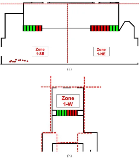
7.2 Geometry of “Noisy-Champs” station - pedestrian navigation . . . 196
7.2.1 Entrance/exit: Zone 1 . . . 198
7.2.2 Access to platforms: Zone 2 . . . 198
7.2.3 Boarding/alighting- Zone 3 . . . 198 7.3 Activities . . . 200 7.3.1 Zone 1 . . . 200 7.3.2 Zones 2 and 3. . . 200 7.4 Traffic organization . . . 202 7.5 Passenger flow . . . 202 7.5.1 Passenger demand . . . 202
7.5.2 Pedestrian distribution along the train platform. . . 203
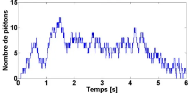
7.5.3 Pedestrian enter volume . . . 204
7.6 Results. . . 205
7.7 Conclusion . . . 207
8 Modeling the lateral pedestrian force on a rigid floor by a self-sustained oscillator 211 8.1 Introduction. . . 212
8.2 Modeling the lateral walking force of a pedestrian on a rigid floor . . . 212
8.2.1 Description of the laboratory experiment . . . 212
8.2.2 Fourier analysis of the lateral walking force . . . 212
8.2.3 Study of the pedestrian lateral force as a function of displacement and velocity. . 219
8.2.4 A self sustained oscillator for the modeling of the lateral pedestrian force . . . 221
8.3 Conclusion . . . 226
8.4 Appendix . . . 229
8.4.1 Lateral walking frequency . . . 229
8.4.2 C1, C3, and ∆1,3 . . . 230
8.4.3 Amplitude of displacement . . . 230
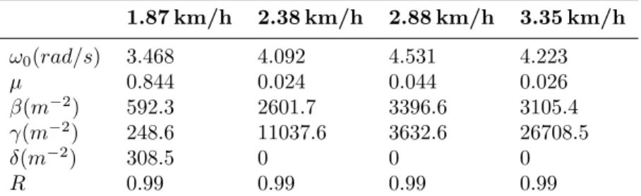
8.4.4 Identified parameters of the proposed oscillator . . . 230
2.1 Exemple d’une simulation d’´evacuation de salle r´ealis´ee avec un mod`ele d’automate
cellu-laire [13]. . . 37
2.2 Les forces agissant sur le pi´eton i.. . . 38
2.3 Deux pi´etons en groupe `al’aide d’un lien existant entre eux. . . 39
2.4 Trajectoires de deux pi´etons identiques i et j se d´epla¸cant dans des directions oppos´ees, pour des valeurs diff´erentes de τ. Apr`es la collision, pour chaque pi´eton, la force d’acc´el´eration int´erieure permet de modifier progressivement la vitesse r´eelle apr`es le choc pour retrouver la vitesse souhait´ee. La rapidit´e du changement de vitesse d´epend des valeurs de τi et τj. Dans cet exemple, τi= τj= τ. . . . 41
2.5 Interaction pi´eton-pi´eton sans force r´epulsive: les repr´esentations `a gauche montrent le mouvement d’un pi´eton apr`es une collision pour (haut) ζi= 1 et (bas) ζi= 0, o`u θd,i= 0. A droite, la rotation du pi´eton est trac´ee en fonction du temps. . . 42
2.6 Variation de ˙θ0 en fonction de log10(Ktg) . . . 43
2.7 Variation de θmax en fonction de ˙θ0et k . . . 43
2.8 S(x) obtenu pour (a) V (x) = 1 partout et (b) V (x) = 1/50 pr`es des murs. . . . 44
2.9 Trajectoire d’un pi´eton pour (a) V (x) = 1 partout et (b) V (x) = 1/50 pr`es des murs. . . 45
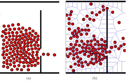
2.10 Discretisation de l’environnement `a l’aide d’un diagramme de Vorono¨ı. . . 45
2.11 D´epˆot de ph´eromones attirant de plus en plus de fourmis vers la source de nourriture. . . 46
2.12 Evolution de la simulation en utilisant un champ de vitesses (a) statique (chemin plus court) et (b) dynamique (chemin plus rapide).. . . 46
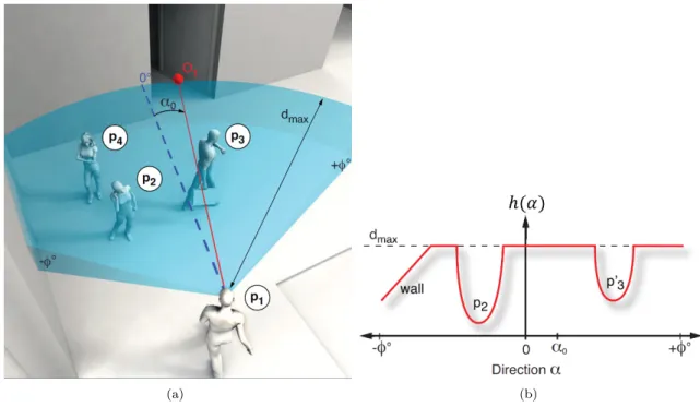
2.13 Interaction pi´eton-pi´eton (a) sans et (b) avec force r´epuslive (pour A = 2000 N et B = 0.08 m) 47 2.14 (a) Illustration d’un pi´eton p1 ayant 3 pi´etons dans son champ de vision et essayant de rejoindre la porte marqu´ee par le point rouge. (b) Repr´esentation graphique de la fonction h(α) [39]. . . . 48
2.15 Deux pi´etons i et j face `a face se croisant. . . . 48
2.16 Fonction h(α) d´efinie par une parabole centr´ee au point (αj, hj). . . 49
2.17 Champs de vision discr´etis´e du pi´eton i. . . . 49
2.18 Distance avant collision - deux pi´etons face `a face se croisant. La m´ethode 1 (en bleu) et la m´ethode 2 (en rouge). . . 50
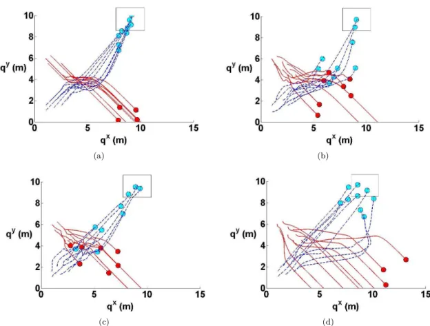
2.19 Croisement de deux groupes de pi´etons: (a) sans ´evitement, (b) ´evitement avec force r´epulsive et ´evitement avec approche cognitive avec (c) la m´ethode 1 et (d) la m´ethode 2. 51 2.20 Croisement de deux groupes de pi´etons: nombre de collisions pour les diff´erentes versions du mod`ele et pour differents nombres de pi´etons. . . 51
2.21 Croisement de deux groupes de pi´etons: temps de calcul pour les diff´erentes versions du mod`ele et pour diff´erents nombres de pi´etons (temps de simulation = 9 s). . . 52
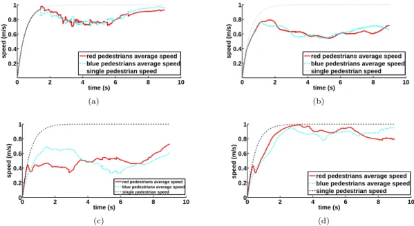
2.22 La vitesse souhait´ee moyenne pour 18 pi´etons pour les diff´erentes versions du mod`ele. . . 52 2.23 Environnement de l’exp´erience (a) r´eelle et (b) mod´elis´e pour les simulations num´eriques. 53
16 LIST OF FIGURES
2.24 Surface repr´esentant εT en fonction de A et B. La fonction exponentielle, repr´esent´ee par
la courbe noire, a pour equation A = 1501 ∗ e−7.98B . . . . 54
2.25 Valeurs du flux sp´ecifique donn´ees par notre mod`ele avec force r´epulsive et celles obtenues exp´erimentalement [41] pour N= (a) 20, (b) 40, et (c) 60. . . 55
2.26 Effets significativement influents dans l’ordre d´ecroissant en prenant en compte les inter-actions jusqu’`a l’ordre 6. . . 58
2.27 Effets principaux du plan d’exp´erience 213. . . . . 59
2.28 Interactions d’ordre 2 des facteurs du plan d’exp´erience 213. . . . . 59
2.29 Valeur de R2 pour chacun des 12 mod`eles construits. . . . . 60
2.30 Vue a´erienne de la gare de Noisy-Champs. . . 61
2.31 Entr´ees-sorties de la gare de Noisy-champs cot´e (a) est et (b) ouest. . . 61
2.32 Quai de la gare de Noisy-Champs (direction Paris).. . . 62
2.33 Scenario de la simulation num´erique. . . 62
2.34 La r´epartition spatiale des voyageurs sur le quai. . . 64
2.35 Passagers entrant dans la gare, achetant leurs billets et passant par les portiques pour acc´eder au quai.. . . 65
2.36 Passagers (a) attendant le train sur le quai et (b) embarquant/d´ebarquant. . . 65
2.37 Nombre de passagers mont´es et descendus, avec le temps d’´echange correspondant, pour chaque porte du train. . . 66
2.38 Demande au niveau des portiques du cot´e sud de la zone 1 de la gare. . . 66
2.39 Installation exp´erimentale [47]. . . 68
2.40 Pi´eton 1-msc : ´evolution temporelle de la force lat´erale pour quatre vitesses de marche diff´erentes. Mesure vs. S´erie de Fourier (ligne en gras) . . . 68
2.41 Pi´eton 1-fmn : ´evolution temporelle de la force lat´erale pour quatre vitesses de marche diff´erentes. Mesure vs. S´erie de Fourier (ligne en gras) . . . 69
2.42 S´erie de Fourier de la force, de la vitesse et du d´eplacement du pi´eton 1-msc pour quatre vitesses de marche diff´erentes pour un cycle : Fy(t) − uy(t) (gauche) et Fy(t) − ˙uy(t) (droite) 70 2.43 S´erie de Fourier de la force, de la vitesse et du d´eplacement du pi´eton 1-fmn pour quatre vitesses de marche diff´erentes pour un cycle : Fy(t) − uy(t) (gauche) et Fy(t) − uy(t) (droite) 70 2.44 Oscillations lat´erales du pi´eton 1-msc. Mod`ele VdPM (croix) vs. s´erie de Fourier (ligne continue): La force lat´erale (gauche), la vitesse lat´erale (centre) et le d´eplacement lat´eral (droite) . . . 72
2.45 Oscillations lat´erales du pi´eton 1-fmn. Le Mod`ele VdPM (croix) vs. s´erie de Fourier (ligne continue): La force lat´erale (gauche), la vitesse lat´erale (centre) et le d´eplacement lat´eral (droite) . . . 72
2.46 Oscillation lat´erale du pi´eton 1-msc. Mod`ele VdPM (croix) vs. S´erie de Fourier (ligne continue): Cycle limite dans le plan de phase (gauche); Diagramme param´etrique 3D avec d´eplacement, vitesse et force lat´erale (droite) . . . 73
2.47 Oscillation lat´erale du pi´eton 1-fmn. Le Mod`ele VdPM (croix) vs. S´erie de Fourier (ligne continue): Cycle limite dans le plan de phase (gauche); Diagramme param´etrique 3D avec d´eplacement, vitesse et force lat´erale (droite) . . . 73
2.48 Oscillation lat´erale du pi´eton 1-msc. Mod`ele VdPM (croix) vs. S´erie de Fourier (ligne continue): la s´erie de Fourier de la force, de la vitesse et du d´eplacement du pi´eton 1-msc pour quatre vitesses de marche diff´erentes pour un cycle Fy(t) − uy(t) (gauche) et Fy(t) − ˙uy(t) (droite). . . 74
2.49 Oscillation lat´erale du pi´eton 1-fmn. Mod`ele VdPM (croix) vs. S´erie de Fourier (ligne continue): la s´erie de Fourier de la force, de la vitesse et du d´eplacement du pi´eton 1-fmn pour quatre vitesses de marche diff´erentes pour un cycle Fy(t) − uy(t) (gauche) et Fy(t) − ˙uy(t) (droite). . . 74
2.50 Param`etres du mod`ele VdPM pour les pi´etons masculins . . . 75
2.51 Param`etres du mod`ele VdPM pour les pi´etons f´eminins. . . 75
3.1 Von-Neumann neighborhood (left), Moore neighborhood (middle), and Hexagonal neigh-borhood (right) [17]. . . 84
automata [16], (b) circular, (c) elliptical or (d) anisotropic form for the social force model [29] and (e) the dynamic form that changes in length (hence the black arrow) proposed by
[19]. . . 87
3.5 Two holding hands pedestrians - Example of linked shoulders . . . 89
3.6 Pedestrian-pedestrian interaction without repulsive forces: the left column shows the pedestrian’s movement after “collision” for ζi = 1 (top) and ζi = 0 (bottom), where θd,i= 0. The right column is a plot of the pedestrian’s rotation as a function of time . . . 92
3.7 Two colliding pedestrians. The dotted line represents each pedestrian’s current walking direction . . . 93
3.8 Velocity after head on collision of two particles for (a) m1 = m2 = 62 kg and | u−1 |=| u−2 |= 1 m/s and (b) m1= 62 kg, m2= 20 kg, | u−1 |= 2 m/s and | u − 2 |= 0.5 m/s . . . 94
3.9 Variation of ˙θ0 as a function of log10(Ktg) . . . 94
3.10 Variation of θmax as a function of ˙θ0 and k . . . 95
4.1 Pedestrian trajectories for a bottleneck . . . 102
4.2 Value function W (t, x) for pedestrians performing an activity located at the head of the arrow [19]. The optimal paths are perpendicular to the iso-value function curves. . . 106
4.3 An illustration of (a) an environment with walls and two obstacles and (b) the correspond-ing static field S(x). . . . 107
4.4 The direction from any point x towards the exit of the environment shown in Fig. 4.3(a) 107 4.5 The red agents move from the green to the red zone while the blue agents head to the middle of the large room. The figure shows the different behavior when using a (left) static potential and (right) a dynamic one [24]. . . 108
4.6 By considering densities (dynamic floor field-right), unnatural congestions (static floor field-left) can be avoided [12]. . . 109
4.7 An example of a navigation graph [35]. . . 109
4.8 An illustration of the multi-scale model setup [36]. . . 110
4.9 Using the dynamic floor field, the pedestrian to the left avoids the congestion even without having a ‘visual’ evidence that it exists [36]. . . 110
4.10 Ped 1 takes route a even though the congestion on routes b and c aren’t important [36]. . 111
4.11 An example of (a) an environment and the corresponding (b) network mapping [40]. . . . 112
4.12 1000 pedestrians distributed in four blocks [40]. . . 112
4.13 Simulation of an evacuation of 1000 pedestrians using (a) the local shortest path, (b) the local shortest with quickest path, (c) the global shortest path, and (d) the global shortest with quickest path [40]. . . 113
4.14 Maps showing the (a)shortest and (b) the “happiest” paths between Euston Square and Tate Modern in London [41]. . . 114
4.15 S(x) obtained for (a) 1/V (x) = 1 s/m everywhere and Dshy = 0 cm and (b) 1/V (x) = 50 s/m near walls for Dshy= 35 cm and the corresponding directing unit vectors towards toward the shortest path for (c) 1/V (x) = 1 s/m everywhere and Dshy = 0 cm and (d) 1/V (x) = 50 s/m near walls for Dshy= 35 cm. . . . 115
4.16 The trajectory of an agent for (a) 1/V (x) = 1 s/m everywhere and Dshy= 0 cm and (b) 1/V (x) = 50 s/m near walls for Dshy= 35 cm. . . . 115
4.17 The effect of Dshy on pedestrians’ trajectories. The dotted line joins the initial and final position of the pedestrian and the solid lines are his/her trajectories for different values of Dshy. . . 116
18 LIST OF FIGURES
4.19 The funnel shape upstream a bottleneck obtained (a) in an experiment [47] and (b) by our model. . . 117 4.20 Bottleneck evacuation: (a) the initial pedestrian positions and (b) the probability of finding
a pedestrian at position x. The black solid lines in (b) are the boundaries of the bottleneck and the the dotted lines represent the two main lanes that formed inside it. The width of each lane is taken equal to the diameter of the disk representing each pedestrian (diami=
diam= 0.46 m). . . . 118
4.21 The influence of the chosen size of the exit area on pedestrian trajectories: (a) the dotted line is the trajectory of the agent for exit area 1 and (b) is the one for exit area 2. . . 118 4.22 Bottleneck evacuation for exit area 2: (a) the initial pedestrian positions and (b) the
probability of finding a pedestrian at position x. The black solid lines in (b) are the boundaries of the bottleneck and the dotted lines represent the two main lanes that formed inside it. The width of each lane is taken equal to the diameter of the disk representing each pedestrian (diami = diam = 0.46 m). . . . 119
4.23 A Cellular automaton [51].. . . 119 4.24 The nodes occupied by a disk of radius 0.23 m representing a pedestrian. . . . 120 4.25 The quickest path around an immobile pedestrian: If V (x, t) is modified only for the
red node (see Fig.4.24), (a) the change in the direction of the unit vectors pointing to the quickest path is insignificant and (b) a collision takes place instead of overtaking. The pedestrian to the left is mobile and the one to the right is immobile. The blue line represents the trajectory of the mobile pedestrian. . . 120 4.26 The quickest path around an immobile pedestrian: If V (x, t) is modified for the area
occupied by each pedestrian i represented by a disk of radius ri, (a) the change in the
direction of the unit vectors pointing to the quickest path is significant but (b) not enough for the mobile pedestrian to overtake the immobile one. The blue line represents the trajectory of the mobile pedestrian. . . 121 4.27 The quickest path around an immobile pedestrian: If V (x, t) is modified for an area that is
double the one occupied by a pedestrian, (a) the change in the direction of the unit vectors pointing to the quickest path is significant and (b) not enough for the mobile pedestrian to overtake the immobile one. The blue line represents the trajectory of the mobile pedestrian.121 4.28 The quickest path around a group of immobile pedestrians: If V (x, t) is modified for an
area that is double the one occupied by a pedestrian, (a) the change in the direction of the unit vectors pointing to the quickest path is significant but (b) not enough for the mobile pedestrian to overtake the immobile group. The blue line represents the trajectory of the mobile pedestrian. . . 122 4.29 The discretization of an environment using a Voronoi diagram. . . 122 4.30 The discretization of an environment with 20 pedestrians using a Voronoi diagram. . . 123 4.31 The quickest path around a group of immobile pedestrians: If V (x, t) is modified for an
area that is double the one occupied by a pedestrian, (a) the change in the direction of the unit vectors pointing to the quickest path is significant and (b) enough for the mobile pedestrian to overtake the immobile group. The red line represents the trajectory of the mobile pedestrian. . . 123 4.32 Spreading pheromone on the path that leads to the food source to attract more ants.. . . 124 4.33 The static floor field for (a) t=0 and (b) t=60. The state of the system at (c) t=0 and (d)
t=60. . . 125 4.34 The dynamic floor field for (a) t=0 and (b) t=60. The state of the system at (c) t=0 and
(d) t=60. . . 126 4.35 Moving around a 180◦ corner using (a) a static floor field and a (b) dynamic one. . . . . . 126
4.36 A pedestrian’s interaction with its surrounding [54]. . . 126 5.1 A collective behavior by (a) a school of fish [2] and (b) a flock of birds (©Owen Humphreys).132 5.2 Two systems using (a) a centralized and (b) a decentralized mechanism [1]. . . 133 5.3 The four steps for studying self-organized collective behavior according to [16]. . . 134 5.4 Indirect interactions between pedestrians create new paths [39]. . . 137
stop-and-go phenomenon throug the propagation of two successive waves (from 1a to 1d then from 2a to 2d). The pilgrims move from left to right. The green color indicates the
pedestrians that are moving [59]. . . 141
5.12 Pedestrian-pedestrian interaction (a) without and (b) with introducing the repulsive force (for A = 2000 N and B = 0.08 m) . . . 143
5.13 The direction of the social repulsive force for two pedestrians. . . 145
5.14 Pedestrian-pedestrian interaction (a) without and (b) with introducing the repulsive force (for A = 2000 N and B = 0.08 m) . . . 145
5.15 (a) Illustration of a pedestrian p1 facing three other subjects and trying to reach the destination point marked in red. The blue dashed line corresponds to the line of sight and (b) a graphical representation of the function h(α) reflecting the distance to collision in direction α[77]. . . . 147
5.16 The distance to destination d(α). . . . 148
5.17 Head on encounter between pedestrians i and j. . . . 149
5.18 Representing Hj(α) by a parabolic function with a vertex at (αj, hj). . . 150
5.19 Discretized vision field of pedestrian i. . . . 150
5.20 Head-on encounter between 2 pedestrians: the distance before collision obtained by method 1 (blue) and method 2 (red). . . 151
5.21 Head-on encounter between two pedestrians: (a) collision model, (b) social repulsive force model, and cognitive model (c) method 1 and (d) method 2.. . . 152
5.22 Overtaking of a moving pedestrian : (a) collision model, (b) social repulsive force model, and cognitive model (c) method 1 and (d) method 2. . . 153
5.23 Overtaking of two immobile pedestrians : (a) collision model, (b) social repulsive force model, and cognitive model (c) method 1 and (d) method 2.. . . 154
5.24 Intersection of 2 pedestrian streams: (a) collision model, (b) social repulsive force model, and cognitive model (c) method 1 and (d) method 2. . . 155
5.25 Intersection of 2 pedestrian streams : number of collisions, with the different models and an increasing number of pedestrians. . . 156
5.26 Intersection of 2 pedestrian streams : computation time, with the different models and an increasing number of pedestrians (Simulation time = 9 s). . . 156
5.27 Intersection of 2 pedestrian streams: (a) collision model, (b) social repulsive force model, and cognitive model (c) method 1 and (d) method 2. . . 157
5.28 The static floor field used to create the queuing area that leads to the service point. . . . 158
5.29 Queuing behavior using (a) repulsive forces and (b) behavioral heuristics. . . 159
6.1 Love Parade in Duisburg Germany [18] and a metro station in Paris during a strike of metro drivers [15]. . . 168
6.2 Development cycle of a simulation model. . . 168
6.3 Quantitative validation using flow [58] and density values [7]. Strategy 0 and Strategy 1 in (a) refer to direction choice strategies [58]. . . 172
6.4 Fundamental diagrams for pedestrian movement in planar facilities. Lines refer to specifi-cations in planning guidelines PM [50]; SFPE [41] and WM [61]. Data points are obtained from experimental measurements (Older, 1968) [44] and [17] . . . 172
6.5 Fit of the simulations performed of the modified model [45] and comparison with the original one, experimental data given by Weidmann [61] and Mori et al.[36] and design data [41]. Error bars represent two standard deviations. . . 173 6.6 Experimental setup (a) and the configuration of 60 pedestrians reproduced by our model (b)175
20 LIST OF FIGURES
6.7 Values of Js obtained with or without introducing the rotation for N= (a) 20, (b) 40 and
(c) 60. The social force is not considered . . . 176
6.8 The surface representing εT as a function of A and B. The curve is given by the exponential function A = 1501 ∗ e−7.98B . . . . 178
6.9 Specific flow measurements obtained by our model (considering the social repulsive force) in comparison with empirical data [57] for N= (a) 20, (b) 40, and (c) 60 . . . 178
6.10 Density measurements for 60 pedestrians obtained by the experiment [57] and by our model (A = 790 kg.m.s−2, B = 0.08 m): (a) density in front of the entrance of the bottleneck and (b) density inside the bottleneck . . . 179
6.11 Flow values obtained by the 2D discrete model (A = 790 N, B = 0.08 m) compared to the experimental data [57] for N = (a) 20, (b) 40, and (c) 60. . . 180
6.12 The probability of finding a pedestrian at position x for 50 runs with N = 60, A = 790 N, B = 0.08 m, and b= (a) 0.8, (b) 0.9, (c) 1, (d) 1.1 and (e) 1.2 . . . 181
6.13 Pedestrian behavior when N = 40 at t = 2.5 s (a) without and (a) with the social repulsive force . . . 182
6.14 The steps of validating a meta model. . . 182
6.15 The bottleneck configuration to be used for the experiments. . . 183
6.16 The terms of the 6thorder model in decreasing order of significance. . . . . 186
6.17 Illustration of the main effects of the 213complete factorial design. . . . . 186
6.18 Illustration of the 2-factor interactions of the main effects of the 213 complete factorial design. . . 187
6.19 The value of R2for each regression model where each time the terms up to a certain order of interactions is considered. . . 188
7.1 The actual RER lines of ile-de-France. . . 196
7.2 The new lines of the Grand Paris Express project. . . 197
7.3 Data requirements for pedestrian simulation in transit stations. . . 197
7.4 Aerial view of “Noisy-Champs” station. . . 197
7.5 Entrance/exit areas of Noisy-Champs : (a) eastern and (b) western sides. . . 198
7.6 Platform (direction Paris) of “Noisy-Champs”: (a) real and (b) modeled.. . . 199
7.7 Zone 3 which is the train (a) real and (b) modeled. . . 199
7.8 Queuing behavior: (a) type 1, (b) type 2, (c) type 3, and (d) type4). . . 200
7.9 Pedestrians entering the train station, buying tickets, and passing the turnstiles to head to the platform. . . 201
7.10 Pedestrians (a)waiting for the train on the platform and (b) boarding/alighting. . . 201
7.11 Train frequency for “Noisy-Champs” station. . . 202
7.12 Simulation scenario. . . 202
7.13 Origins of passengers alighting the train at “Noisy-Champs”.. . . 203
7.14 Destinations of passengers boarding the train at “Noisy-Champs”.. . . 203
7.15 Pedestrian distribution along the train platform for “Noisy-Champs” train station for the east-west direction. . . 204
7.16 Simulation scenario with passenger flow data. . . 206
7.17 Number of embarked and disembarked passengers and the corresponding exchange time for each door of the train. . . 206
7.18 Demand on the turnstiles of the south eastern side of the train station.. . . 206
8.1 Experimental setup [6]. . . 213
8.2 Modulus of ˆFy (Eq.(8.1)) for the lateral force of pedestrian 1-msc for different walking velocities. . . 214
8.3 Modulus of ˆFy (Eq.(8.1)) for the lateral force of pedestrian 1-fmn for different walking velocities. . . 214
8.4 Time-histories of the lateral force of pedestrian 1-msc for different walking speeds. Exper-imental results (thin line) vs. truncated Fourier Series (Eq. 8.5, thick line). . . 215
8.5 Time-histories of the lateral force of pedestrian 1-fmn for different walking speeds. Exper-imental results (thin line) vs. truncated Fourier Series (Eq. 8.5, thick line). . . 216
8.9 Fourier series for 2 different walking velocities for pedestrian 1-msc : the lateral force Fy(t)
(left), the lateral velocity vy(t) = ˙uy(t) (center), and the lateral displacement uy(t) (right) 220
8.10 Fourier series for 2 different walking velocities for pedestrian 1-fmn : the lateral force Fy(t)
(left), the lateral velocity vy(t) = ˙uy(t) (center), and the lateral displacement uy(t) (right) 221
8.11 Amplitude of the maximum displacement for 4 different walking velocities for (a) the male and (b) female participants. . . 221 8.12 Fourier series approximation of the lateral force, velocity and displacement for pedestrian
1-msc for two walking velocities.The phase plot (left) and the lateral force as a function of displacement and velocity (right).. . . 222 8.13 Fourier series approximation of the lateral force, velocity and displacement for pedestrian
1-fmn for two walking velocities.The phase plot (left) and the lateral force as a function of displacement and velocity (right).. . . 222 8.14 Experimental phase plots for 4 different walking velocities of (a) the male and (b) female
participants.. . . 223 8.15 Fourier series of the force, velocity and displacement for one cycle for pedestrian 1-msc :
Fy(t) − uy(t) (left) and Fy(t) − uy(t) (right). . . . 224
8.16 Fourier series of the force, velocity and displacement for one cycle for pedestrian 1-fmn :
Fy(t) − uy(t) (left) and Fy(t) − uy(t) (right). . . . 224
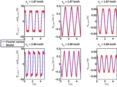
8.17 Lateral oscillation of the pedestrian 1-msc. Model (cross symbol) vs. truncated Fourier series results (solid line): the lateral force (left), velocity (middle), and displacement (right).225 8.18 Lateral oscillation of the pedestrian 1-fmn. Model (cross symbol) vs. truncated Fourier
series results (solid line): the lateral force (left), velocity (middle), and displacement (right).226 8.19 Lateral oscillations of the pedestrian 1-msc. Model (cross symbol) vs. truncated Fourier
series results (solid line) over one cycle. The limit cycle in the phase-plane (left) and the lateral force as a function of displacement and velocity (right). . . 226 8.20 Lateral oscillations of the pedestrian 1-fmn. Model (cross symbol) vs. truncated Fourier
series results (solid line) over one cycle. The limit cycle in the phase-plane (left) and the lateral force as a function of displacements and velocity (right). . . 227 8.21 Force-displacement and force-velocity diagrams for pedestrian 1-msc over one cycle.
Trun-cated Fourier series (solid line) vs. model results (cross symbol). Parametric plot Fy(t) −
uy(t) (left) and Fy(t) − uy(t) (right). . . . 227
8.22 Force-displacement and force-velocity diagrams for pedestrian 1-fmn over one cycle. Trun-cated Fourier series (solid line) vs. model results (cross symbol). Parametric plot Fy(t) −
uy(t) (left) and Fy(t) − uy(t) (right). . . . 228
8.23 Identified model parameters for all of the male participants. . . 228 8.24 Identified model parameters for all of the female participants. . . 229 8.25 Lateral walking frequency as a function of height for (a) the male and (b) female participants.229 8.26 Lateral walking frequency as a function of BMI for (a) the male and (b) female participants.230 8.27 Lateral walking frequency as a function of mass for (a) the male and (b) female participants.230 8.28 Fourier series approximation of the lateral walking force of the male participants: the
amplitudes C1, C3, and the phase difference ∆ϕ1,3 as a function of their height. The
average values are represented by the dotted lines. . . 231 8.29 Fourier series approximation of the lateral walking force of the male participants: the
amplitudes C1, C3, and the phase difference ∆ϕ1,3 as a function of their mass. The
22 LIST OF FIGURES
8.30 Fourier series approximation of the lateral walking force of the male participants: the amplitudes C1, C3, and the phase difference ∆ϕ1,3 as a function of their BMI. The average
values are represented by the dotted lines. . . 232 8.31 Fourier series approximation of the lateral walking force of the female participants: the
amplitudes C1, C3, and the phase difference ∆ϕ1,3 as a function of their height. The
average values are represented by the dotted lines. . . 232 8.32 Fourier series approximation of the lateral walking force of the female participants: the
amplitudes C1, C3, and the phase difference ∆ϕ1,3 as a function of their mass. The average
values are represented by the dotted lines. . . 233 8.33 Fourier series approximation of the lateral walking force of the female participants: the
amplitudes C1, C3, and the phase difference ∆ϕ1,3 as a function of their BMI. The average
values are represented by the dotted lines. . . 233 8.34 Amplitude of the maximum displacement as a function of height for (a) the male and (b)
female participants.. . . 234 8.35 Amplitude of the maximum displacement as a function of their BMI for (a) the male and
(b) female participants. . . 234 8.36 Amplitude of the maximum displacement as a function of mass for (a) the male and (b)
female participants.. . . 235 8.37 Identified parameters of the mVdP model as a function of height for (a) the male and (b)
female participants.. . . 236 8.38 Identified parameters of the mVdP model as a function of BMI for (a) the male and (b)
female participants.. . . 237 8.39 Identified parameters of the mVdP model as a function of mass for (a) the male and (b)
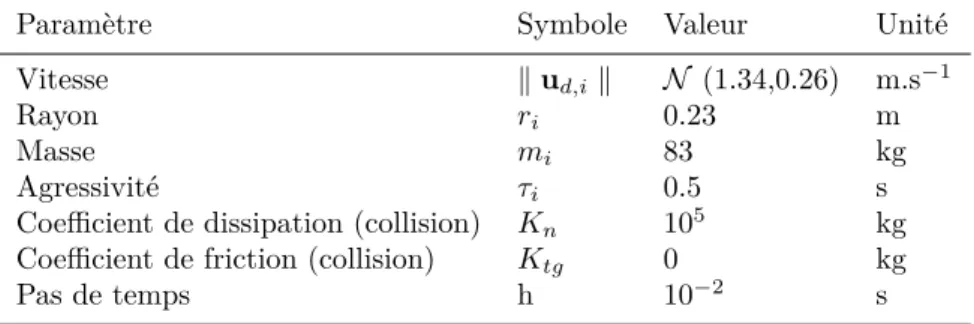
2.2 Valeurs des param`etres fix´es dans les simulations num´eriques. . . 54 2.3 Les facteurs choisis et leurs intervalles de variation. . . 56 2.4 Plan factoriel 213complet. . . . . 56
2.5 Analyse de Yates en utilisant les donn´ees du tableau 2.4. . . 57 2.6 Analyse de variance pour le plan factoriel 213. . . . . 57
2.7 Tableau de l’analyse de variance (ANOVA). . . 60 2.8 Flux des voyageurs descendant `a Noisy-Champs . . . 63 2.9 Flux des voyageurs montant `a Noisy-Champs. . . 63 2.10 Temps de stationnement des trains `a quai `a la gare de Noisy-Champs. . . 66 2.11 Masse et taille des 20 participants masculins. . . 67 2.12 Masse et taille des 11 participantes f´eminines. . . 67 2.13 Param`etres du mod`ele VdPM du pi´eton 1-msc. . . 71 2.14 Param`etres du mod`ele VdPM du pi´eton 1-fmn. . . 71 3.1 Typical parameter values for the social-force model [10]. . . 86 4.1 Shy away distance of pedestrians . . . 117 5.1 Different values of the desired speed. . . 136 6.1 Examples of possible experimental data for the validation of the main core components of
building evacuation models. . . 171 6.2 Experimental specific flow Js,exp (individuals.m−1.s−1) [57]. The time interval ∆t is the
time measured between the passage of the first person and the last one. . . 175 6.3 Parameters used in the simulations for pedestrian flow through a bottleneck . . . 177 6.4 Norms of residuals of the linear regressions plotted in Fig. 6.11 . . . 179 6.5 The factors and their levels. . . 183 6.6 The obtained 213 full factorial design. . . . . 184
6.7 Yates method of analysis using the data from Table 6.6. . . 185 6.8 Analysis of variance table for the 213factorial design. . . . . 185
6.9 The ANOVA table. . . 188 7.1 Flow of pedestrians alighting at “Noisy-Champs” . . . 203 7.2 Flow of pedestrians boarding at “Noisy-Champs” . . . 204 7.3 Distribution of pedestrians alighting at “Noisy-Champs” for each of the three zones. . . . 204 7.4 An example of the pedestrian enter volume from the eastern entrance of “Noisy-Champs”
train station. . . 205 7.5 Train dwell times in the “Noisy-Champs” station. . . 206 8.1 Mass and height of the 20 male participants. . . 213
24 LIST OF TABLES
8.2 Mass and height of the 11 female participants. . . 214 8.8 Fourier analysis of the lateral walking force for the female pedestrians : the average values
of the dynamic load factors (DLF) of the odd harmonics up to the 9thorder for 4 different
walking velocities. . . 216 8.3 Fourier series for pedestrian 1-msc : fundamental frequency, amplitudes and phase
differ-ence for the odd harmonics up to the 9thorder for four walking velocities. . . . . 217
8.4 Fourier series for pedestrian 1-fmn : fundamental frequency, amplitudes and phase differ-ence for the odd harmonics up to the 9thorder for four walking velocities. . . . . 217
8.5 Fourier analysis of the lateral walking force for the male participants: average values and standard deviations of the fundamental frequency, amplitudes and phase differences of the odd harmonics up to the 9th order for 4 walking velocities.. . . . 217
8.6 Fourier analysis of the lateral walking force for the female participants: average values of the fundamental frequency, amplitudes and phase differences of the odd harmonics up to the 9thorder for 4 walking velocities.. . . . 218
8.7 Fourier analysis of the lateral walking force for the male pedestrians: the average values of the dynamic load factors (DLF) of the odd harmonics up to the 9thorder for 4 different
walking velocities. . . 218 8.9 Hybrid Van der Pol/Rayleigh oscillator with the γ-term: the identified parameters
associ-ated with pedestrian 1-msc. . . 225 8.10 Hybrid Van der Pol/Rayleigh oscillator with the γ-term: the identified parameters
˙θi(t) rotational velocity of a pedestrian ri radius of a pedestrian
mi mass of a pedestrian
ud,i desired speed of a pedestrian
u∗ optimal speed according to a particular strategy la
i restoring torque ki torsional stiffness ci rotational damping
h(α) the distance before the first collision in the direction α dmax the range of the pedestrians’ vision field
αi,0 the direction of the destination point θi(t) orientation of a pedestrian about the ez-axis τi relaxation time
λ reflects the anisotropic nature of the force Ii moment of inertia
A maximum value of the magnitude of the social repulsion force B fall-off length of the social repulsion force
G center of the disk representing a pedestrian M inertial matrix
N number of pedestrians in a certain environment Nc number of contacts or collisions
Nsubgroup number of pedestrians who belong to a group
Kn dissipation coefficient for the normal component of the dissipative percussion Ktg dissipation coefficient for the tangential component of the dissipative percussion Kv coefficient of viscous dissipation
T velocity field
D dynamic velocity field S static velocity field V wavefront velocity J flow for a given facility
Js specific flow for a given facility
Φ pseudo-potential of dissipation
ui(t) velocity vector of a pedestrian
fa acceleration force fsoc social repulsion force fphys physical contact force
ed,i unit vector of the desired direction of a pedestrian
26 LIST OF TABLES
ud,i desired velocity vector of a pedestrian
fext exterior force vector fint interior force vector
pint interior percussions pext exterior percussions
enij a unit vector pointing from pedestrian i to j q[t,T ) trajectory of a pedestrian between instants t and T
u[t,T ) control path or the velocity on a certain trajectory between instants t and T
u∗ optimal velocity according to a particular strategy e∗ optimal direction according to a particular strategy
1.1 Crowd Management-History. . . . 28 1.2 What is a crowd? . . . . 29 1.3 Why simulate crowd motion and evacuation processes? . . . . 30
28 1.1. CROWD MANAGEMENT-HISTORY
1.1
Crowd Management-History
The history of crowd management is not very recent. In ancient Rome, the architects and builders of the Flavian Amphitheater, or Colosseum designed and built the biggest arena in the world at that time, capable of holding between 50,000 - 80,000 people not to mention the wild animals such as elephants and tall giraffes. They came up with an ingenious system of entrances, corridors, and staircases that allowed the crowds to enter, be seated and exit the Colosseum quickly, easily and efficiently. To solve the problem of crowd control, 80 separate entrance arches were made (see Fig. 1.1)so that the Colosseum could be cleared in less than 10 minutes [1]. These entrances lead to a corridor that spans uninterruptedly around the building leading to staircases and passages to the seats. However, the crowd management methods that were used gave very little importance for the well-being of the audience. Nowadays, crowd management has become a scientific study where crowd dynamics, crowd psychology, and staff training all contribute in ensuring the safety of crowds.
Figure 1.1: The architectural plan of the Flavian amphitheather or the colosseum [2].
In the scope of this work, we are interested in studying crowd dynamics. Crowd dynamics is about studying the formation and displacement of crowds for densities above one person per square meter. Since at high densities individual safety becomes at risk, understanding the dynamics of crowds, how pedestrians understand and interpret information, and how their behavior is affected by management systems is crucial and form the basis of the science of crowd dynamics [3]. A more commonly used term than the science of crowd dynamics is the “Crowd Science” which includes the science of crowd dynamics, psychology and behavior. The broad definition of this domain is Crowd Modeling, Monitoring and Management. Three topics aimed at developing crowd management plans with safer and more robust standards.
The objective of crowd modeling is to model how pedestrians behave and crowds form and move. Its use has become crucial since it is thought that the major contributing factor in crowd related disasters is the lack of understanding of crowd dynamics and crowd psychology [3]. For this reason, pedestrians have been the subject of several empirical studies since 4 decades now [4–6]. The obtained direct observations, photographs, and time-lapse films were used as the main evaluation methods. The main objective of these studies was to develop a level-of-service concept [7], design elements of pedestrian facilities [8–10], or planning guidelines [11]. With more complex architecture, large facilities and events, these studies have become insufficient to evaluate the evacuation of challenging situations. As a result, a number of simulation models were developed such as the queuing models [12], transition matrix models [13], stochastic models [14], and models for the route choice behavior of pedestrians [15].
However, these models failed to take into account the self-organization phenomena occurring in pedes-trians crowds. The first model that was able to reproduce spatio-temporal patterns of motion was pro-posed by Henderson [16, 17] who used principles from the fluid-dynamic theory. While this approach could be partially confirmed, it is does not take into consideration certain particular interactions (i.e. avoidance and deceleration maneuvers) that does not obey momentum and energy conservation. The attention was then shifted to modeling individual pedestrian motion. Agent-based modeling is now the main focus of pedestrian research. The most well-known types of agent-based models are the force-based
Crowds are not to be considered as homogeneous entities since they are made up of several individuals with different motives. According to empirical data gathered by scientists, crowds are more of a process (see Fig. 1.2)- they have a beginning, middle and end [28]. The cognitive and social processes involved in crowd movement allows us to describe it on different levels [29]:
• Physical/physiological • Psychological
• social
Figure 1.2: Crowd is a process of assembling, gathering and dispersing [30].
Pedestrian behavior is related to the psychological and social level. This behavior is not the same in groups as in crowds making it important to distinguish between the two. A group is formed by two or more individuals. A large group is called a mass. Only when this group occupy a single location and share a common focus, does it form a crowd (see Fig. 1.3).
Figure 1.3: Classification of crowds [31]. Crowds are large groups that occupy a single location and share a common focus.
30 1.3. WHY SIMULATE CROWD MOTION AND EVACUATION PROCESSES?
1.3
Why simulate crowd motion and evacuation processes?
Over the last decade, the field of pedestrian movement has received growing interest. This has been due to several reasons.
• Growing mobility: walking is inevitable. It is necessary for every other form of traveling (e.g., walking to the bus, car, train platform, airport terminal,...). In addition, it is probably one of the most time-intensive form of mobility [29]. Simulation can help increase the level of comfort for pedestrians and decrease the waiting times by assessing the design of facilities.
• Large facilities: more and more large facilities (e.g., shopping centers, theme parks, stadiums, ...) are being built destined to accommodate large crowds. This can result in densely packed crowds that create high pressure that poses a threat to people’s health. Therefore, detailed planning of the walkways and crowd management are crucial to ensure a safe and comfortable environment for large crowds.
• Large events: large events such as rallies, marches, parades, or rock concerts usually attract a huge number of people. To manage crowds safely, a deep knowledge of the laws of crowd motion is necessary. Scientific research helps acquire the knowledge needed to channel flows, increase capacity by decreasing orientation problems or holding back people (creating waiting areas) to avoid peak flows in critical areas.
• Emergency evacuations: by using simulations, buildings or passenger vessels’ (e.g., ships, airplanes) layouts can be improved and optimized so that they can be evacuated in a short time even under stress conditions.
• Safety requirements: new passenger vessels are being designed to carry more and more people. This is being accompanied with additional and more strict safety requirements.
• Collective motion: to increase our knowledge on crowd motion, it is important to understand the principles and mechanisms behind collective motion and self-organization phenomena such as shock waves, oscillation at bottlenecks, lane formation, etc.
• Crowd related disasters: the use of crowd modeling has become crucial since it is thought that the major contributing factor in crowd related disasters is the lack of understanding of crowd dynamics and crowd psychology [32]. Table1.1shows that the numerical analysis of flow rates, fill times and capacity are potentially the primary elements where improvements to crowd safety would have most impact [32]. While writing this dissertation, one of deadliest disasters in years to hit the Muslim Hajj in Saudi Arabia [33] happened where at least 717 people died and hundreds of others hurt in a stampede of pilgrims outside Mecca.
For all of the above reasons, it is necessary to study the laws of crowd motion and what influences it especially in urgent evacuations. Computer simulations seem to be the best tool to investigate crowd movement and assess evacuation processes. The potential areas of application are numerous: buildings, urban systems like pedestrian crossings, buses, trains, aircrafts, ships, shopping malls, theme parks, railway and subway stations airports, etc.
The outline of this thesis is divided into 8 chapters. In the second chapter, an extended abstract of all the thesis is done in french. The accomplished work and the obtained results in this PhD thesis are briefly presented. In the third chapter, an overview of crowd modeling is given. The two main approaches to modeling pedestrian movement are explained followed by a survey on the three main types of models that exist in literature. Our discrete model is then introduced and positioned with respect to other works. The new modifications that have been done to the model are demonstrated.
The fourth chapter is dedicated to pedestrian navigation and route choice. The first part of the chapter assesses the different types of classification of pedestrian navigation levels and the existing route choice models. In the second part, the different displacement strategies that have been developed in our model are demonstrated. Their influences on the overall crowd dynamics are compared.
In the fifth chapter, pedestrian-pedestrian interactions are addressed. The effect and the importance of pedestrian interactions at the microscopic level on the overall crowd dynamics on the macroscopic level
Table 1.1: Incidents related to crowd events [32].
Year Casualties Cause Place
1989 96 dead, 400 injured (too many people) Design (throughput) Hillsborough, UK
1990 1426 pilgrims crushed (too many people) Design (throughput) Mina Valley, Saudi Arabia
1994 266 pilgrims crushed, 98 injured (too many people) Design (throughput) Jamarat, Saudi Arabia
1996 83 crushed, 180 injured (too many people) Information (Forged Tickets) Guatemala City 1997 22 pilgrims crushed, 43 injured (too many people) Design (throughput) Jamarat, Saudi Arabia
1998 118 pilgrims crushed, 434 injured (too many people) Design (throughput) Jamarat, Saudi Arabia
1999 51 killed, 150 injured in stampede (reaction) Information (Weather) Kerala, India 1999 53 killed, 190 injured in stampede (reaction) Information (Weather) Minsk, Belarus 2001 35 pilgrims crushed, 179 injured (too many people) Design (throughput) Jamarat, Saudi Arabia
2001 4 dead, including 3 children (reaction) Information (Handouts - crazing) Aracaju, Brazil 2002 10 trampled, Mall crowd craze (reaction) Information (Handouts - crazing) Yakohama, Hapan 2004 249 pilgrims crushed, 252 injured (too many people) Design (throughput) Jamarat, Saudi Arabia
2004 37 dead , 15 injured in crowd crush (too many people) Design (throughput) Beijing, China
2006 363 dead, 389 injured in crowd crush (reaction) Design (throughput) Jamarat, Saudi Arabia
2006 74 dead, 300 injured in crowd crush (reaction) Design (throughput) Manila, Philippines
2006 51 dead, 238 injured in crowd crush (reaction) Information (political rally) Yemen, Middle East 2008 146 dead, 50 injured in stampede (narrow road) Design (throughput) Himachal Pradesh, India
2008 23 dead, dozens injured in Ramadan (reaction) Information (handouts) Pasuran, Java
2008 1 dead, 4 injured - store sales (reaction) Information (Black Friday sales) Wal-Mart, New York, USA 2009 22 dead, 132 injured - football (reaction) Design (throughput) Abidjan, Ivory Coast
2009 60 injured, 4 hospitalized (JLS) (reaction) Design (capacity) Birmingham (JLS), UK
2010 26 dead, 55 injured (too many people) Design (Throughput) Timbuktu, Mali, West Africa
2010 63 dead, 44 injured (too many people - narrow road) Design (throughput) Kunda, North India
2010 10 police officers injured (reaction) (too many people) Design (capacity+crazing)
2010 60 injured (reaction) Information (screamer) Amesterdam, The Netherlands 2010 14 injured (too many people at entry gates) Information (forged tickets) Johannesburg, South Africa 2010 Over 100 injured (reaction) Design (choice of barriers) EDC - Los Angeles, USA
2010 21 dead, 511 injured (too many peopl) Design (throughput) Duisburg, Germany
2010 10 dead, dozens injured (reaction) Information (over reaction) Bihar, India 2010 7 dead, 70 injured (reaction) Information (rain stopped) Nairobi, Kenya 2010 347 dead, 395 injured (too many people) Design (capacity) Phnom Penh, Cambodia
2011 102 dead, 44 injured (too many people) Design (capacity) Kerala, India
2011 11 dead, 29 injured (reaction) Information (shots fired) Port Harcourt, Nigeria 2011 36 dead, 70 injured (too many people) Design (capacity) Bamako, Mali
2011 7 dead, 30 injured (too many people) Design (capacity) Brazzaville, Congo
2011 2 dead, 13 injured (too many people) Information (poor ticket allocation) Jakarta, Indonesia 2012 1 dead, 13 injured (too many people) Design (throughput) Johannesburg, South Africa
2012 74 dead, over 1000 injured (too many people + rioting) Design (throughput) + riot Port Said, Egypt 2012 3 dead, dozens injured (too many people) Design (throughput) Cairo (copic), Egypt
32 1.3. WHY SIMULATE CROWD MOTION AND EVACUATION PROCESSES? is first explained through the concept of self-organization phenomena. The types of pedestrian behaviors and interactions that were integrated into our model are shown. The methods that we used to model these behaviors are then compared using several criteria.
The sixth chapter concerns the validation and verification (V&V) of pedestrian models. First, a bibliographical study on the different V&V methods available in literature is carried out. Then, an experimental design is used in order to identify the input parameters of our model that significantly influence the flow values for the case of a bottleneck. Finally, for the same previous case, the capacity of our model to reproduce experimental results is examined.
The seventh chapter is dedicated to a study on modeling pedestrian flows in the Noisy-Champs train station in ˆıle-de-France. In the first place, the methods that were used to obtain the geometrical, train, and pedestrian data is shown. These data were then used to create a simulation scenario and to model pedestrian movement in the aforementioned train station. The obtained results are then compared to observations.
In the last chapter, the hybrid version of the Van der Pol self-sustained oscillator that is developed to model the lateral walking force of a pedestrian on a rigid floor is further validated by processing the experimental data of 31 pedestrians walking on a treadmill. In addition, the obtained results of the male and female participants are compared to identify the differences.
[3] G. K. Still, Crowd dynamics. PhD thesis, University of Warwick, 2000.
[4] B. D. Hankin and R. A. Wright, “Passenger flow in subways,” OR, vol. 9, pp. 81–88, June 1958. [5] S. Older, “Movement of pedestrians on footways in shopping streets,” Traffic Engineering and
Con-trol, vol. 10, pp. 160–163, 1968.
[6] U. Weidmann, “Transporttechnik der fußg¨anger,” report Schriftenreihe Ivt- Berichte 90, ETH Z¨urich, 1993.
[7] J. J. Fruin, “Designing for pedestrians: a level of service concept,” in Highway research record, 1971. [8] J. Pauls, “The movement of people in buildings and design solutions for means of egress,” Fire
Technology, vol. 20, pp. 27–47, Feb. 1984.
[9] D. Helbing, Verkehrsdynamik. Berlin, Heidelberg: Springer Berlin Heidelberg, 1997.
[10] D. Helbing, L. Buzna, A. Johansson, and T. Werner, “Self-organized pedestrian crowd dynamics: experiments, simulations, and design solutions,” Transportation Science, vol. 39, pp. 1–24, Feb. 2005. [11] Highway capacity manual. Washington, D.C.: Transportation Research Board, lslf sub ed., Dec.
1994.
[12] S. J. Y. Jr and J. M. Smith, “Modeling circulation systems in buildings using state dependent queueing models,” Queueing Systems, vol. 4, pp. 319–338, Dec. 1989.
[13] D. Garbrecht, “Describing pedestrian and car trips by transition matrices,” Traffic Quarterly, vol. 27, no. 1, 1973.
[14] N. Ashford, M. O’LEARY, and P. D. McGinity, “Stochastic modelling of passenger and baggage flows through an airport terminal,” Traffic Engineering & Control, vol. 17, no. 5, 1976.
[15] A. Borgers and H. J. P. Timmermans, “City centre entry points, store location patterns and pedes-trian route choice behaviour: A microlevel simulation model,” Socio-Economic Planning Sciences, vol. 20, no. 1, pp. 25–31, 1986.
[16] L. Henderson, “The statistics of crowd fluids,” vol. Nature,229, pp. 381–383, 1971.
[17] L. F. Henderson, “On the fluid mechanics of human crowd motion,” Transportation Research, vol. 8, pp. 509–515, Dec. 1974.
[18] M. Chraibi, A. Seyfried, and A. Schadschneider, “Generalized centrifugal-force model for pedestrian dynamics,” Physical Review E, vol. 82, no. 4, p. 046111, 2010.
34 BIBLIOGRAPHY [19] D. Helbing and P. Moln`ar, “Social force model for pedestrian dynamics,” Physical Review E, vol. 51,
pp. 4282–4286, May 1995.
[20] R. L¨ohner, “On the modeling of pedestrian motion,” Applied Mathematical Modelling, vol. 34, pp. 366–382, Feb. 2010.
[21] W. J. Yu, R. Chen, L. Y. Dong, and S. Q. Dai, “Centrifugal force model for pedestrian dynamics,”
Physical Review E, vol. 72, p. 026112, Aug. 2005.
[22] A. Kirchner and A. Schadschneider, “Simulation of evacuation processes using a bionics-inspired cellular automaton model for pedestrian dynamics,” Physica A: Statistical Mechanics and its
Appli-cations, vol. 312, pp. 260–276, Sept. 2002.
[23] M. Fukui and Y. Ishibashi, “Jamming transition in cellular automaton models for pedestrians on passageway,” Journal of the Physical Society of Japan, vol. 68, no. 11, pp. 3738–3739, 1999. [24] V. Blue and J. Adler, “Emergent fundamental pedestrian flows from cellular automata
microsimu-lation,” Transportation Research Record: Journal of the Transportation Research Board, vol. 1644, pp. 29–36, Jan. 1998.
[25] C. Burstedde, K. Klauck, A. Schadschneider, and J. Zittartz, “Simulation of pedestrian dynamics using a two-dimensional cellular automaton,” Physica A: Statistical Mechanics and its Applications, vol. 295, no. 3, pp. 507–525, 2001.
[26] S. Gopal and T. R. Smith, “Human way-finding in an urban environment: a performance analysis of a computational process model,” Environment and Planning A, vol. 22, no. 2, pp. 169 – 191, 1990. [27] C. W. Reynolds, “Evolution of corridor following behavior in a noisy world,” From animals to
animats, vol. 3, pp. 402–410, 1994.
[28] J. M. Kenny, C. McPhail, P. Waddington, S. Heal, S. Ijames, D. N. Farrer, J. Taylor, and D. Oden-thal, “Crowd behavior, crowd control, and the use of non-lethal weapons,” tech. rep., DTIC Docu-ment, 2001.
[29] H. L. Kl¨uepfel, A cellular automaton model for crowd movement and egress simulation. PhD thesis, Universit¨at Duisburg-Essen, Fakult¨at f¨ur Physik, 2003.
[30] A. Hunsicker, Behind the Shield: Anti-Riot Operations Guide. Universal-Publishers, 2011. [31] D. Forsyth, Group Dynamics 3rd. Wadsworth, Belmont, CA, 1998.
[32] “PhD - Crowd cynamics | Prof. Dr. G. Keith Still,” 1990.
[33] A. A. O. i. Hofuf, S. Arabia, S. D. i. Amman, and Jordan, “More Than 700 People Killed in Mecca Stampede,” Wall Street Journal, Sept. 2015.
![Figure 2.25: Valeurs du flux sp´ecifique donn´ees par notre mod`ele avec force r´epulsive et celles obtenues exp´erimentalement [ 41 ] pour N= (a) 20, (b) 40, et (c) 60](https://thumb-eu.123doks.com/thumbv2/123doknet/2597780.57249/56.892.146.730.138.614/figure-valeurs-flux-ecifique-force-epulsive-obtenues-erimentalement.webp)