ECOLE DE TECHNOLOGIE SUPÉRIEURE UNIVERSITÉ DU QUÉBEC
MANUSCRIPT-BASED THESIS PRESENTED TO ÉCOLE DE TECHNOLOGIE SUPÉRIEURE
IN PARTIAL FULFILLEMENT OF THE REQUIREMENTS FOR THE DEGREE OF DOCTOR OF PHILOSOPHY
Ph. D.
BY
Roberto Salvador FÉLIX PATRÓN
OPTIMIZATION OF THE VERTICAL FLIGHT PROFILE ON THE FLIGHT MANAGEMENT SYSTEM FOR GREEN AIRCRAFT
MONTREAL, DECEMBER 15TH, 2014
© Copyright
Reproduction, saving or sharing of the content of this document, in whole or in part, is prohibited. A reader who wishes to print this document or save it on any medium must first obtain the author’s permission.
BOARD OF EXAMINERS (THESIS PH.D.)
THIS THESIS HAS BEEN EVALUATED
BY THE FOLLOWING BOARD OF EXAMINERS
Dr. Ruxandra Mihaela Botez, Thesis Supervisor
Department of Automated Production Engineering at École de technologie supérieure
Dr. Lyne Woodward, Chair, President of the Committee
Department of Automated Production Engineering at École de technologie supérieure Dr. Marc Paquet, Member of the Committee
Department of Electrical Engineering at École de technologie supérieure
Dr. Youmin Zhang, External Examiner
Department of Mechanical and Industrial Engineering at Concordia University
THIS THESIS WAS PRENSENTED AND DEFENDED
IN THE PRESENCE OF A BOARD OF EXAMINERS AND THE PUBLIC DECEMBER 2ND, 2014
ACKNOWLEDGMENTS
First and foremost, I would like to thank my supervisor Ruxandra Botez for her guidance throughout the duration of my research project, and for her constant motivation to my participation at academic events. Thanks are due to her for encouraging us to start conversations during the networking events and thus, improving our communication skills, and for the corrections brought to my writings.
Acknowledgments are dues to:
The Green Aviation Research & Development Network (GARDN), CMC Electronics – Esterline, CONACYT and the FRQNT for their financial support.
Oscar and Georges, for sharing their wisdom and experiences during these years.
Vanessa and Tamara, who inspired me to initiate my Ph.D. studies.
Alejandro Murrieta, colleague and friend since the beginning of my Ph.D., for listening and criticizing all of my ideas, for participating actively on the development each one of my algorithms and for being always the first one to read my drafts.
All of the members of LARCASE who participated on this research project. Julián, Jocelyn, Romain, Margaux. To my coauthors who participated in the development of the optimization algorithms: Aniss, Adrien, Marine, and especially, Yolène.
To my roommates Nicolás and Jonathan, who not only had to live with me for over two years, but also helped me to improve my French communication skills.
Finally, I want to thank my mother, Cecilia, who has always supported me from Mexico and that without her, I would never be where I am, nor be the person that I am today.
OPTIMIZATION OF THE VERTICAL FLIGHT PROFILE ON THE FLIGHT MANAGEMENT SYSTEM FOR GREEN AIRCRAFT
Roberto Salvador FÉLIX PATRÓN ABSTRACT
To reduce aircraft’s fuel consumption, a new method to calculate flight trajectories to be implemented in commercial Flight Management Systems has been developed. The aircraft’s model was obtained from a flight performance database, which included experimental flight data. The optimized trajectories for three different commercial aircraft have been analyzed and developed in this thesis.
To obtain the optimal flight trajectory that reduces the global flight cost, the vertical and the LNAV profiles have been studied and analyzed to find the aircraft’s available speeds, possible flight altitudes and alternative horizontal trajectories that could reduce the global fuel consumption. A dynamic weather model has been implemented to improve the precision of the algorithm. This weather model calculates the speed and direction of wind, and the outside air temperature from a public weather database.
To reduce the calculation time, different time-optimization algorithms have been implemented, such as the Golden Section search method, and different types of genetic algorithms. The optimization algorithm calculates the aircraft trajectory considering the departure and arrival airport coordinates, the aircraft parameters, the in-flight restrictions such as speeds, altitudes and WPs. The final output is given in terms of the flight time, fuel consumption and global flight cost of the complete flight.
To validate the optimization algorithm results, the software FlightSIM® has been used. This software considers a complete aircraft aerodynamic model for its simulations, giving results that are accurate and very close to reality.
OPTIMISATION DU PROFIL VERTICAL DE VOL DANS LES SYSTÈMES DE GESTION DE VOL POUR LES AVIONS VERTS
Roberto Salvador FÉLIX PATRÓN RÉSUMÉ
Une nouvelle méthode pour calculer des trajectoires de vol pouvant être implémentée dans un système de gestion de vol a été développée pour réduire la consommation de carburant des avions. Le modèle des avions a été obtenu à partir d’une base de données de performances, composée de données expérimentales de vol. Cette thèse présente l’analyse et le développement de trajectoires optimisées pour trois types d’avions commerciaux.
Afin d’obtenir la trajectoire de vol optimale réduisant le coût global du vol, les profils vertical et latéral de navigation ont été étudiés. Une analyse complète des vitesses disponibles a été effectuée, ainsi qu’une analyse des altitudes de vol possibles et des trajectoires horizontales alternatives qui peuvent aider à réduire la consommation globale de carburant. Un modèle dynamique de la météo a été implémenté afin d’améliorer la précision de l’algorithme. Ce modèle de la météo calcule la direction et la vitesse du vent, ainsi que la température de l’air à partir d’une base de données publique.
Dans le but de réduire le temps de calcul, différents algorithmes d’optimisation ont été implémentés, tels que la méthode de la section d’or ainsi que différents types d’algorithmes génétiques. Les algorithmes d’optimisation calculent la trajectoire de l’avion en considérant les coordonnées des aéroports de départ et d’arrivée, les paramètres de l’avion, et les restrictions pendant le vol comme la vitesse, l’altitude et les points de cheminement. Le résultat global de l’algorithme est donné en termes de temps de vol, carburant consommé et coût global de vol pour un vol complet.
Le logiciel FlightSIM® a été utilisé pour valider les résultats obtenus par les algorithmes d’optimisation. Ce logiciel considère un modèle aérodynamique complet des avions, ce qui produit des résultats précis et très proches de la réalité.
TABLE OF CONTENTS
Page
INTRODUCTION ...1
0.1 Statement of the problem ...1
0.2 Objectives ...5
0.3 Methodology ...6
0.3.1 Aircraft model - Performance database ... 6
0.3.2 Dynamic weather model ... 8
0.3.3 Time-optimization algorithms ... 8
CHAPTER 1 LITERATURE REVIEW ...11
1.1 Aviation’s fuel burn reduction ...11
1.2 Flight trajectory optimization ...12
1.3 Calculation time optimization algorithms ...15
CHAPTER 2 APPROACH AND ORGANIZATION OF THE THESIS ...17
CHAPTER 3 ARTICLE 1: NEW ALTITUDE OPTIMIZATION ALGORITHM FOR A FLIGHT MANAGEMENT SYSTEM PLATFORM IMPROVEMENT ON COMMERCIAL AIRCRAFT ...23 3.1 Introduction ...24 3.2 Global cost ...27 3.3 Methodology ...28 3.4 Climb...32 3.5 Cruise ...35 3.6 Descent ...39 3.7 Results ...42 3.8 Conclusions ...47
CHAPTER 4 ARTICLE 2: HORIZONTAL FLIGHT TRAJECTORIES OPTIMIZATION FOR COMMERCIAL AIRCRAFT THROUGH A FLIGHT MANAGEMENT SYSTEM ...49
4.1 Introduction ...50
4.2 Methodology ...54
4.2.1 Aircraft PDB ... 54
4.2.2 The grid ... 55
4.2.3 Inputs and outputs ... 59
4.2.4 Weather model ... 60
4.2.5 The genetic algorithm ... 61
4.2.5.1 Individuals and initial population ... 62
4.2.5.2 Evaluation ... 63
4.2.5.3 Selection ... 63
4.3 Results ...68
4.4 Conclusion ...76
CHAPTER 5 ARTICLE 3: NEW METHODS OF OPTIMIZATION OF THE FLIGHT PROFILES FOR PERFORMANCE DATABASE-MODELED AIRCRAFT .77 5.1 Introduction ...78
5.2 Methodology ...82
5.2.1 Aircraft model – Performance database ... 82
5.2.2 Wind model and flight cost equation ... 84
5.2.2.1 Wind model ... 84 5.2.2.2 Flight cost... 87 5.2.3 Climb... 88 5.2.4 Cruise ... 89 5.2.4.1 LNAV ... 90 5.2.4.2 VNAV ... 94 5.2.5 Descent ... 95 5.3 Results ...97 5.4 Conclusions ...102
CHAPTER 6 ARTICLE 4: FLIGHT TRAJECTORY OPTIMIZATION THROUGH GENETIC ALGORITHMS COUPLING VERTICAL AND LATERAL PROFILES ...105
6.1 Introduction ...106
6.2 Methodology ...110
6.2.1 Aircraft model – performance database ... 111
6.2.2 Dynamic wind model ... 114
6.2.3 The grid ... 117
6.2.4 The genetic algorithm ... 117
6.2.4.1 Individuals and initial population ... 118
6.2.4.2 Evaluation ... 119
6.2.4.3 Selection ... 120
6.2.4.4 Reproduction ... 121
6.3 Results ...122
6.3.1 The genetic algorithm ... 122
6.3.2 Fuel cost reduction ... 126
6.4 Conclusions ...128
DISCUSSION OF RESULTS...129
CONCLUSIONS AND RECOMMENDATIONS ...131
LIST OF TABLES
Page
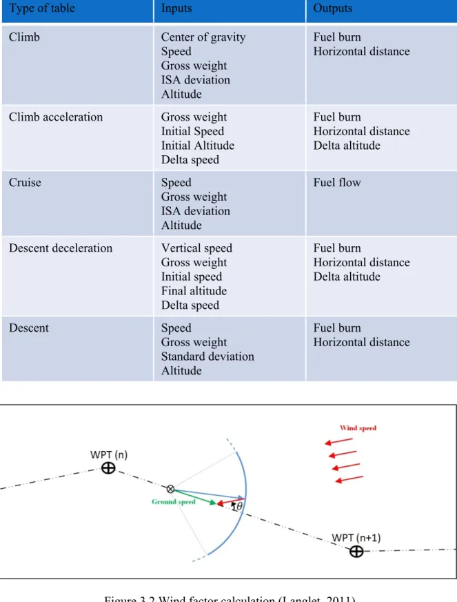
Table 0.1 Inputs and outputs of a typical commercial PDB ...7
Table 3.1 Inputs and outputs for the PDB for a commercial aircraft ...31
Table 3.2 Crossover altitude example for a 300/0.82 speed schedule ...33
Table 3.3 Crossover altitudes table (ft) ...34
Table 3.4 Fuel burn precision analysis with FlightSIM® ...43
Table 3.5 Flight time precision analysis with FlightSIM® ...43
Table 3.6 Speed only optimization comparison for the mid-range aircraft ...45
Table 3.7 Speed and altitude optimization comparison for the mid-range aircraft ...46
Table 4.1 Example of the latitudes and longitudes for a grid ...57
Table 4.2 Inputs and outputs for the trajectories’ optimization algorithm ...59
Table 4.3 Flight tests from real weather data obtained from Environment Canada with 9 WPs and 5% of initial population ...70
Table 4.4 Flight tests for the variation of the initial population, with a separation angle of 15º and 9 WPs ...72
Table 4.5 Calculation times for different number of WPs and initial population with a separation angle of 15º and 9 WPs ...73
Table 4.6 Flight tests with 12 WPs and a 5% initial population ...74
Table 4.7 Flight tests for different separation angles ...75
Table 5.1 Inputs and outputs of the PDB ...83
Table 5.2 Example of individual’s crossover ...94
Table 5.3 Fuel burnt and flight time for a Lisbon to Toronto flight ...99
Table 5.4 Fuel burnt and flight time for a London to Toronto flight ...101
Table 5.5 Optimization results from the proposed algorithm ...102
Table 6.2 Individuals parameters for the GA ...119 Table 6.3 Number of possible trajectories within the 3D grid varying
the number of SCs and WPs ...124 Table 6.4 GA optimization results ...126 Table 6.5 Flight cost reduction results ...127
LIST OF FIGURES
Page
Figure 0.1 CI influence on the climb technique (Airbus, 1998) ...2
Figure 0.2 Optimal altitude variation with the aircraft gross weight (Airbus, 1998) ...3
Figure 0.3 Speed and altitude variation with the CI (Airbus, 1998) ...3
Figure 0.4 Climb profiles (Airbus, 2004) ...4
Figure 0.5 SC versus continuous climb (Airbus, 2004) ...4
Figure 0.6 Wind influence on fuel consumption and flight time (Airbus, 2004) ...5
Figure 3.1 Example of information given on the PDB ...30
Figure 3.2 Wind factor calculation (Langlet, 2011) ...31
Figure 3.3 Climb phase ...34
Figure 3.4 Golden section method flowchart ...38
Figure 3.5 Cruise phase (flights over 500 nm) ...39
Figure 3.6 Descent ...39
Figure 3.7 Descent flowchart ...41
Figure 3.8 Global cost error variation with CI ...44
Figure 4.1 PDB format ...55
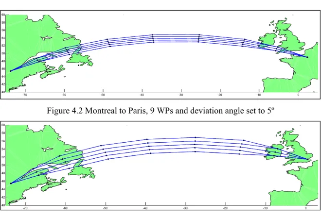
Figure 4.2 Montreal to Paris, 9 WPs and deviation angle set to 5º ...56
Figure 4.3 Montreal to London, 9 WPs and deviation angle set to 10º ...56
Figure 4.4 Grid example for a flight from Madrid to Rome ...57
Figure 4.5 Example of a flight trajectory presented on the grid (3,3,3,2,2,3,4,4,3) ...58
Figure 4.6 Example of an invalid trajectory on the grid ...58
Figure 4.7 Representation of the roulette wheel selection ...64
Figure 4.8 Example of reproduction with a GA ...66
Figure 4.10 GA diagram ...67
Figure 5.1 Example of the PDB ...84
Figure 5.2 Airspeed, crosswind and effective wind ...85
Figure 5.3 Wind factor calculation (Langlet, 2011) ...86
Figure 5.4 Wind interpolation method (Langlet, 2011) ...87
Figure 5.5 Climb trajectory example ...89
Figure 5.6 In-cruise grid example of a Paris to Montreal flight ...90
Figure 5.7 Grid numbering example for a westbound flight ...91
Figure 5.8 Roulette wheel selection example ...93
Figure 5.9 In-cruise SCs ...95
Figure 5.10 Descent trajectory example ...96
Figure 5.11 Optimization algorithm diagram ...97
Figure 5.12 VNAV flight from Lisbon to Toronto ...99
Figure 5.13 LNAV flight from Lisbon to Toronto ...100
Figure 5.14 VNAV flight from London to Toronto ...101
Figure 6.1 Interpolations to obtain the aircraft’s flight performance during climb from the PDB ...112
Figure 6.2 Interpolations to obtain the aircraft’s flight performance during cruise from the PDB ...113
Figure 6.3 Airspeed, crosswind and effective wind ...115
Figure 6.4 Wind factor calculation ...115
Figure 6.5 Wind interpolation method ...116
Figure 6.6 Dynamic diagram to calculate the total number of possibilities in a 2D grid ...123
Figure 6.7 Dynamic diagram example to calculate the total number of possibilities in a 2D grid for 6 WPs ...123
LIST OF ABREVIATIONS
3D PAM 3D Path Arrival Management ATC Air Traffic Control
BADA Base of Aircraft Data
CDA Continuous Descent Approach CI Cost Index
CO2 Carbon dioxide
ETMS Enhanced Traffic Management System FAA Federal Aviation Administration FMS Flight Management System GA Genetic Algorithm
GDPS Global Deterministic Prediction System
GRIB2 General Regularly-Distributed Information, Binary form version IAS Indicated AirSpeed
IATA International Air Transport Association ICAO International Civil Aviation Organization ISA International Standard Atmosphere LNAV Lateral NAVigation
NGATS Next Generation Air Transportation System PDB Performance DataBase
PTT Part-Task Trainer
RTA Required Time of Arrival
SESAR Single European Sky ATM Research TAS True AirSpeed
TOC Top Of Climb TOD Top Of Descent
UTC Coordinated Universal Time VNAV Vertical NAVigation WP WayPoint
INTRODUCTION
0.1 Statement of the problem
The global aviation industry produced 676 million tons of CO2 in 2011, 689 million in 2012,
and 701 million in 2013 (ATAG, 2012; 2013; 2014). This amount represents around 2% of the total emissions produced worldwide. CO2 emissions contribute to global warming, that is
one of the biggest environmental problems encountered today.
In Canada, the Green Aviation Research & Development Network (GARDN) was founded in 2009, undertaking different research and development projects to reduce greenhouse gas emissions. One of the first projects in this network was called “Optimized Descents and Cruise”. The new proposed optimization algorithm was developed in this project, in collaboration between the École de Technologie Supérieure and the avionics company CMC Electronics – Esterline.
A Flight Management System (FMS) is a fundamental avionics element in actual aircraft. This is a system with the main function to reduce the crew workload during flight time, through the automation of many aircraft tasks; the aircraft path planning is one of them.
A FMS receives inputs such as the aircraft’s speed, cruise altitude, the distance to travel and the weather conditions that will provide information for the trajectory creation. The reduction of the fuel burn impact of an aircraft is not limited to consume the least fuel possible, but other variables must also be considered. The Cost Index (CI) is a constant used by the airlines to determine the operating cost of the flight, which includes variables such as the fuel price, the number of crew members working during the flight, and the flight time. It influences directly on the global cost of the flight. A CI close to zero indicates that the operation costs for the flight are low, and thus the flight time importance would also be low. A high CI indicates that the operation cost is high, and the flight time would have to be reduced in order to economize in operation costs.
Figure 0.1 shows the influence of the CI in a climb trajectory in which the FMS calculates the ascent to the TOC (Top Of Climb) position (Airbus, 1998). It should be noted that the higher the CI is, the shorter the trajectory is to the destination point.
Figure 0.1 CI influence on the climb technique (Airbus, 1998)
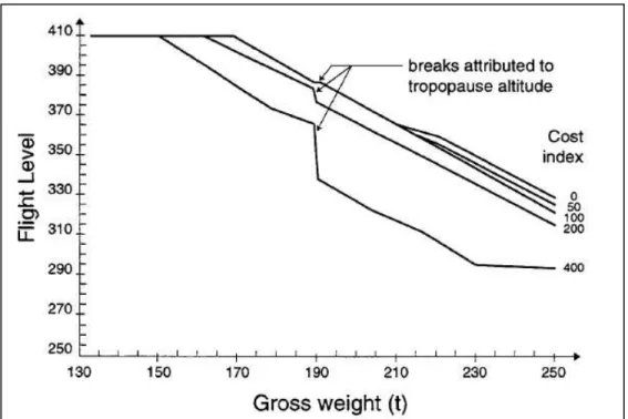
Another important factor to consider when optimizing a trajectory is the aircraft weight; the heavier the aircraft is, the lower the optimal altitude is located. Figure 0.2 shows an example of the relationship between the optimal flight altitude and the aircraft weight. In the absence of winds, this relationship is close to linear. The influence of the CI is also represented on Figure 0.2, where as the CI increases, the optimal flight altitude decreases.
Figure 0.3 shows the relationship between the aircraft speeds and altitudes in terms of the CI for an Airbus A310 aircraft.
As seen on Figure 0.3, the speed, the altitude, the gross weight and the CI are entirely codependent in the search of optimal flight conditions.
3
Figure 0.2 Optimal altitude variation with the aircraft gross weight (Airbus, 1998)
For the initial climb, a constant aircraft speed is selected to climb at a specific altitude, frequently 10,000ft (Airbus, 2004, p. 27). The optimal climb speed is selected in terms of the CI. A slower climb speed will result in a shorter traveled distance and a longer time to reach the final destination, while a higher speed will reduce the time (Figure 0.4) but increase the fuel consumption, and this is the reason why the CI determines the choice of the profile to be used.
Figure 0.4 Climb profiles (Airbus, 2004)
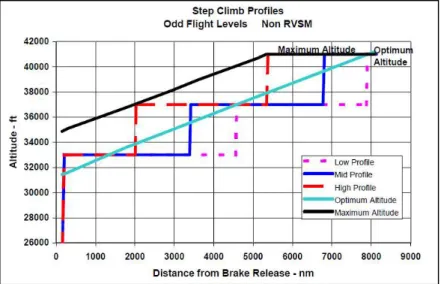
Once the aircraft is in the cruise phase, a Step Climb (SC) or a continuous climb could be made. The continuous climb will provide the maximal fuel economization, as the optimal altitude will be reached quickly. The SC technique is shown on Figure 0.5. SC consists in ascending in steps of 1000ft, 2000ft or 4000ft, each time followed by a cruise phase, instead of climbing in a straight line to a specific altitude.
5
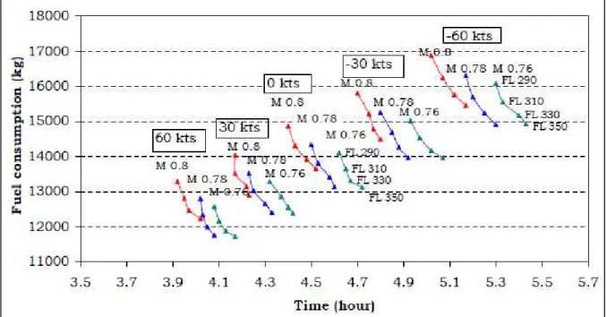
Wind influence is also an important factor to be considered. In Figure 0.6, the fuel consumption and the flight time are shown for a 2000 nm segment with fixed aircraft gross weight, by taking the Airbus A321 as reference. Positive speed values in knots <kt> are considered as tailwinds, while negative wind speed should be taken as headwinds.
Figure 0.6 Wind influence on fuel consumption and flight time (Airbus, 2004)
It can be observed that the stronger the tailwind is, the minimum flight time and fuel burn are obtained. In case of headwinds, it would be necessary to increase the aircraft’s speed to reduce the flight time, thus increasing the fuel burn.
Current FMS platforms do not present a complete optimization of the vertical and lateral flight profiles (VNAV and LNAV).
0.2 Objectives
The global objectives of this project concern the calculation of the optimal LNAV and VNAV profiles in terms of aircraft’s speeds and altitudes, by considering the CI, a complete
analysis of the winds and the variation of the aircraft weight during the flight, in order to reduce the global flight cost.
The global objectives could be divided into the following sub-objectives:
1. Validation of the numerical model of three different commercial aircraft, by comparing its results expressed in terms of aircraft’s fuel burn and flight time with FlightSIM® and the Part-Task Trainer (PTT) from CMC Electronics – Esterline. 2. Calculation of the flight cost for all the possible flight trajectories by performing an
exhaustive computation of the parameters included in the PDB of each aircraft to obtain the speeds and altitudes that reduce the global flight cost (VNAV profile). 3. Development and implementation of a dynamic wind model to calculate the influence
of the wind and outside air temperature during a flight trajectory. 4. Analysis of alternative flight trajectories to optimize the LNAV profile.
5. Implementation of different time-optimization algorithms to reduce the global computation time of the algorithm.
6. Comparison of the flight trajectory optimization algorithm with real flight trajectories in order to reduce the global flight cost.
0.3 Methodology
In this section, an introduction to the numerical aircraft model is defined, followed by the implementation of the dynamic wind model to calculate the cost of the flight trajectories.
0.3.1 Aircraft model – Performance database
The algorithms in this thesis were developed in Matlab®, using the PDB provided by CMC Electronics – Esterline. The PDB is a database of over 30,000 lines containing information on the real performance of different commercial aircraft. The inputs and the outputs contained in these databases are described in Table 0.1. The flight time is calculated from the
7
aircraft’s TAS (True AirSpeed), and the wind influence is calculated with a wind triangle methodology which is explained in the next section. The PDB contains a large quantity of very detailed aircraft information; however, there are five main tables that are used in the development of the algorithms. This information gives the performance (outputs) of each aircraft for different parameters (inputs), at each phase of the flight.
Table 0.1 Inputs and outputs of a typical commercial PDB
To obtain the performance information from the database, the Lagrange linear interpolation method is applied, as shown in Equation (0.1).
= −
− ∗ +
−
− ∗ (0.1)
A complete flight trajectory can be calculated precisely in terms of flight time, distance and fuel burn from Equation (0.1).
Type of table Inputs Outputs
Climb Center of gravity Speed Gross weight ISA deviation Altitude Fuel burn (kg) Horizontal distance (nm) Climb acceleration Gross weight Initial Speed Initial Altitude Delta speed Fuel burn (kg) Horizontal distance (nm) Delta altitude (ft) Cruise Speed Gross weight ISA deviation Altitude Fuel flow (kg/hr) Descent deceleration Vertical speed Gross weight Initial speed Final altitude Delta speed Fuel burn (kg) Horizontal distance (nm) Delta altitude (ft) Descent Speed Gross weight Standard deviation Altitude Fuel burn (kg) Horizontal distance (nm)
0.3.2 Dynamic weather model
The wind data used in this algorithm is extracted from Environment Canada (2013). The information is presented under a Global Deterministic Prediction System (GDPS) format. The GDPS model provides a 601×301 latitude-longitude grid with a resolution of 0.6×0.6 degrees. At each point of this grid, information such as the wind direction, speed, temperature, and pressure can be obtained for different altitudes, in 3-hour time blocks.
The wind directly affects the horizontal distance traveled with respect to ground level, and indirectly affects the fuel consumption. The ground speed is calculated with Equation (0.2) so that it can be considered in the horizontal distance calculation, and is expressed in knots <kt>.
Ground speed = Airspeed + Effective wind speed (0.2) The airspeed is an aircraft’s speed relative to the air mass, and the wind is the horizontal motion of this air mass relative to the ground. The effective wind is the wind’s component of the aircraft’s trajectory, and the crosswind is that component perpendicular to the effective wind speed. The effective wind speed is expressed with Equation (0.3).
Effective wind speed = Real wind - Crosswind (0.3) In the flight cost optimization program, the influence of the wind is calculated dynamically, i.e., it is updated as the aircraft moves in space and time.
0.3.3 Time-optimization algorithms
To reduce the number of calculations, two different methods are implemented in this project: the Golden Section search and Genetic Algorithms (GAs).
9
The “Golden Section” method is a nonlinear optimization method that reduces the search interval by the same fraction, with each iteration, at a golden section ratio, which is commonly known in mathematics as the “golden ratio” (Venkataraman, 2009). This method is applied to calculate the VNAV profile without performing an exhaustive search of all the possible flight parameters found in the PDB, but still obtaining the optimal climb and cruise combination.
GAs were used to reduce the calculation time during the cruise, for the LNAV profile. Alternative trajectories were analyzed through a grid (2D and 3D). Within the grid, the number of possible alternative trajectories increases exponentially as its size increases. The calculation of all the possible alternative trajectories is not only impractical, it is also time-consuming.
CHAPTER 1
LITERATURE REVIEW
1.1 Aviation’s fuel burn reduction
Multiple solutions to reduce aircraft emissions have been put forward. These solutions can be divided in three major categories : aircraft technology improvement, alternative fuels, and improvements in air traffic management and airline operation (Pan, Huang and Wang, 2014). Each of these categories could increase aircraft efficiency and thereby reduce fuel burn and emissions.
One of the research areas in the aircraft technology improvement category is focused on increasing engine efficiency through lighter designs (Williams and Starke, 2003), increased compression rates (Salvat, Batailly and Legrand, 2013) or optimized aerodynamic patterns (Panovsky J, 2000), to name a few. Airlines have been constantly reducing aircraft weight by changing to lighter seats (AirTransat, 2014). Techniques to install more efficient electrical wiring have also been studied (Wattar et al., 2013). Design studies were performed to reduce drag through wing elasticity improvements (Nguyen et al., 2013), wing morphing (Grigorie, Botez and Popov, 2013) or through the aircraft efficiency increasing through the addition of winglets (Freitag and Schulze, 2009).
To reduce its impact on climate change, the aviation industry has been studying sustainable biofuels to provide a cleaner source of fuel (Sandquist and Guell, 2012). Today, the aviation sector uses petroleum-derived liquid fuels, which is not only a limited fuel resource, it also contributes to CO2 emissions. Hendricks, Bushnell and Shouse (2011) performed a study on
biofuels in which they conclude that there is a large productive capacity for biofuels, and also the potential for carbon emission neutrality and reasonable costs. Airline companies, such as Porter (2012), already use a 50:50 biofuel/Jet A1 fuel blend to perform a complete flight, which showed that biofuels are an important option for a greener aviation sector.
1.2 Flight trajectory optimization
Air traffic management and airline operation improvement would also reduce aviation’s environment footprint. Air Traffic Control (ATC) is in charge of assigning the trajectories to airlines; once in-flight, authorization from the ATC is required to perform a trajectory deviation. The FMS is an in-flight device that can be used to identify optimal trajectories to propose to the ATC.
In the mid 1970s, Lockheed developed an FMS to be implemented in their aircraft Tristar-L-1011. Later in the 1980s, other companies started adding the FMS as standard equipment (Avery, 2011). Since then, FMSs have been continuously upgraded and presently all aircraft are equipped with an FMS. The main function of an FMS is to assist the pilot in several tasks, such as navigation, guidance, trajectory prediction and flight path planning.
Even if researchers have been working impetuously on improving FMS, recent studies demonstrated that improvement areas are still vast. Herndon, Cramer and Nicholson (2009) found that many different FMS act differently in terms of optimization and trajectories generation.
Researchers have tried to improve the performance of the FMSs for decades. Lidén (1992) first mentioned that “with no wind, optimal altitude increases nearly linearly with distance as fuel is burned off”. He proposed to include wind and temperature variations on the FMSs to obtain an accurate optimization of the vertical flight profile. A couple of years later, Lidén (1994) defined that FMS would be improved by the optimization of aircraft trajectories in order to avoid air traffic issues. These studies were confirmed later by other researchers.
Hagelauer and Mora-Camino (1998) proposed a dynamic programming algorithm for FMSs to calculate the fuel burned by the aircraft during the flight, in order to obtain an accurate estimation for the creation of onboard trajectories. They were able to solve this problem with an acceptable processing time. Dancila, Botez and Labour (2012; 2013) studied a new
13
method to estimate the fuel burn from aircraft to improve the precision of flight trajectory calculations.
In order to have a more substantial impact on the environment, it is much more indicated to conceive and analyze a trajectory optimization for a full flight considering the climb, cruise and descent.
Many research groups have focused specifically on the descent phase, where the goal is to reduce pollution close to air terminals in terms of both noise pollution and fuel burn emissions. Clarke et al. (2004) introduced the Continuous Descent Approach (CDA) method to reduce noise, which consisted of the deceleration and descent of an aircraft at its own vertical profile from the TOD (Top Of Descent). They presented the design and implementation of an optimized profile descent in high-traffic conditions, as for example at the Los Angeles International Airport (LAX), which increased operational efficiency from traffic management and reduced fuel, emissions and noise (Clarke et al., 2013). Dancila, Botez and Ford (2013) created an analysis tool to estimate the fuel and emissions cost produced by aircraft during a missed approach. Reynolds, Ren and Clarke (2007) concluded that the CDA effectively reduced fuel burn and noise near airports simply by keeping the aircraft at the highest possible altitude before its descent.
For long flights, however, the cruise is the phase where the most significant fuel reduction can be obtained (ATAG, 2014). In fact, 80% of the CO2 emissions produced by aviation
come from long flights (more than 1,500 km or 810 nm). To improve the VNAV (Vertical NAVigation) profile in the cruise phase, the pilot has frequently the possibility in-flight to climb to a different flight level in order to reach the optimal altitude.
Lidén studied the variation of the optimal altitude as fuel is burned during the flight (1992). Murrieta (2013) analyzed the cruise phase to determine a pre-optimal vertical profile and to evaluate the altitudes and speeds around its vicinity. Chakravarty (1985), from a flight aerodynamics perspective, described the variation of the optimal cruise speed with flight
operation costs. Lovegren (2011) analyzed how the fuel burn could be reduced during the cruise phase by choosing the appropriate cruise altitudes and speeds and by performing SCs. Jensen et al. (2013) presented a speed optimization method for the cruise with fixed lateral movement by analyzing radar information from the United States Federal Aviation Administration’s (FAA) Enhanced Traffic Management System (ETMS) (Palacios and Hansman, 2013). Their results show that most flights in the United States do not take place at an optimal speed, which increases their fuel consumption.
The influence of weather on aircraft flight has been considered as part of strategies to take advantage of winds to reduce flight time and/or to avoid headwinds that could also increase global flight costs. Murrieta (2013) presented an algorithm which optimized the vertical and horizontal trajectories by taking into account the wind forces and patterns as well as the variation of the CI. Filippone (2010) analyzed the influence of the cruise altitude on the creation of contrails and on the flight cost. Gagné et al. (2013) performed an exhaustive research of all possible speeds and altitudes to obtain the optimal trajectory and to reduce fuel burn. Bonami et al. (2013) studied a trajectory optimization method capable of guiding an aircraft through different WPs (WayPoints) by considering the wind factors and reducing fuel burn through a multiphase mixed-integer control. Fays and Botez (2013) developed a 4D algorithm treating meteorological conditions or air traffic restrictions in a specified air space, defining them as obstacles in order to improve the FMS’s trajectory-creation capabilities. Franco and Rivas (2011) analyzed the minimal fuel consumption for an airplane at a fixed cruise altitude, using a variable arrival-error cost that penalizes both late and early arrivals. They showed that the minimal cost is obtained when the arrival-error cost is null, and found that the use of different optimal cruise altitudes would obtain the minimal cost/lowest fuel consumption with a fixed estimated arrival time.
However, in order to achieve maximal optimization using all these proposed techniques, an improved method of communication between the FMS and the ATC must be established. Mayer (2006) studied the benefits of an integrated aviation modeling and evaluation platform, in which ATC and the FMS could be coupled to obtain better flight path planning.
15
For both the Next Generation Air Transportation System (NGATS) in the USA, and the Single European Sky ATM Research (SESAR) in Europe, the implementation of Required Time of Arrival (RTA) as a part of the FMS and ATC was an important step towards a better air traffic control. De Smedt and Berz (2007) studied the characteristics of different FMS’ performance to determinate the accuracy of their RTA and the influence it could have on ATC. Friberg’s (2007) study showed that promising results in terms of the environment could be achieved by establishing communication between the FMS’ RTA function and ATC. Air traffic conditions have also been identified as the cause of aircraft missed approaches (Murrieta Mendoza, Botez and Ford, 2014).
In this thesis, a complete flight profile is analyzed, including the climb, cruise and descent, considering both the LNAV and VNAV profiles. These algorithms have been developed to propose an optimal flight trajectory through the FMS to ATC for authorization. The optimization results obtained in this project would still require ATC’s permission to execute the proposed optimal trajectory.
1.3 Calculation time optimization algorithms
Searching among all the different possible trajectories that an aircraft could choose would be ideal to find the optimal trajectory that minimizes the fuel burn, but it would eventually result in a long processing time algorithm. In order to reduce the computing time, different time optimization methods have been applied. These methods reduce the computing time by analyzing a smaller portion of the possible flight trajectories that would converge to the minimal fuel burn trajectory. Stochastic methods were considered as possible solution for solving our optimization problem. The Monte Carlo optimization algorithm proposed by Visintini et al. (2006) applied in ATC systems, would be a reasonable approach to find the aircraft optimal trajectories for fuel burn reduction on aircraft. The Monte Carlo method explores the entire range of solutions (that as it was mentioned before, those are practically
infinite) while following a random path to converge towards the optimum value of the study, in this case, the maximal fuel efficiency trajectory.
The Golden Section search optimization algorithm has been applied to the calculation of the optimal cruise. This is a nonlinear optimization method that reduces the search interval by the same fraction, with each iteration, at a golden section ratio, which is commonly known in mathematics as the golden ratio (Venkataraman, 2009).
GAs have been used in aviation to resolve high complexity problems, and are useful when a solution involving many imposed restrictions is searched. Kanury and Song (2006) used GAs to find the optimal trajectory under the presence of unknown obstacles, obtaining satisfactory results in a short computing time; the optimal route was obtained using their algorithm and the calculation time was reduced. Turgut and Rosen (2012) used GAs to obtain the optimal aircraft descent in terms of the fuel flow values and altitudes to reduce the global descent cost. These algorithms are useful when searching for a solution involving multiple imposed restrictions. Kouba (2010) studied GAs as a means to incorporate several constraints into a trajectory optimization problem, where the objective was to find the shortest route while considering different restrictions.
Different versions of the GAs have been used throughout this thesis in order to reduce the calculation time for the trajectory optimization problem (Félix Patrón, Berrou and Botez, 2014; Félix Patrón et al., 2013; Félix Patrón et al., 2013).
The flight trajectory optimization algorithms proposed in this thesis reduce the fuel burn while the calculation time is optimized.
CHAPTER 2
APPROACH AND ORGANIZATION OF THE THESIS
The research project presented in this thesis could be divided in four main phases:
• Statement of the problem and model validation • Optimization of the VNAV profile
• Optimization of the LNAV profile
• Coupling of both the VNAV and LNAV profiles
During the first phase, all the possible flight trajectories were calculated using the aircrafts PDB through MATLAB®, and the aircraft’s fuel consumption and flight time were obtained. The results obtained with the algorithm were compared with the results obtained by the flight simulator FlightSIM® from Presagis. The results showed that the results were close to reality and the aircraft models were validated.
During the second phase, after the validation of the aircraft models, for a given flight segment, all the possible flight trajectories for a single path (no horizontal deviations) were calculated using an exhaustive search, analyzing all the different available parameters given by the PDB such as aircraft weight, altitude and speeds. The trajectory representing the lowest flight cost was obtained and defined as the “optimal trajectory for the VNAV profile”.
The third phase consisted in the implementation of a weather model into the algorithm. With a complete weather model around the flight route, the algorithm was capable of analyzing possible alternative trajectories to take advantage of the winds aiming to reduce the flight cost. As the trajectory was larger, the number of calculations increased and different time-optimization algorithms were applied. The algorithm analyzed only the cruise phase for long flights, since it is in this phase where an alternative trajectory, even if increasing the actual
flight distance, could help the aircraft to reduce de fuel burn by a correct interpretation of the winds. At a fixed altitude during cruise, the LNAV profile was optimized.
In the fourth and final phase, the optimization for both the VNAV and LNAV were coupled in order to obtain the maximal flight optimization.
As the main author, the research in this thesis was diffused in four journal papers and six conference papers. Three of the journal articles have been published and one is currently under review for publication in peer-review scientific journals. These papers are presented from Chapter 3 to Chapter 6.
Dr. Ruxandra Botez, as a co-author, supervised the realization of all the presented research. In the second paper, the internship student Aniss Kessaci worked as a co-author by implementing the GA used to reduce calculation time. In the third paper, the internship student Yolène Berrou created the method to calculate weather dynamically and the coupling of both LNAV and VNAV algorithms. Mr. Dominique Labour, a co-author from the company CMC Electronics – Esterline, worked in-house on the experimental validation of the project developed by our academic team.
In Chapter 3, the research paper entitled “New altitude optimization algorithm for a Flight Management System platform improvement on commercial aircraft” (Félix Patrón, Botez and Labour, 2013), was published in The Aeronautical Journal, in August 2013.
This paper presents an introduction to the trajectory optimization subject. In this paper, the aircraft has been numerically modeled through the PDB using Matlab®. It includes a description of the parameters considered during the flight to calculate the flight trajectories, and includes a complete calculation of each flight trajectory. A description is made of how the climb, cruise and descent are calculated.
19
The flight cost results obtained by the proposed algorithm are compared with the simulator FlightSIM® results to validate the model of the aircraft. Then, the results obtained with the in-house algorithm were compared with the PTT results, which represent a commercial FMS from the company CMC Electronics. At this point, only the VNAV profile was analyzed.
The algorithm calculated the cost for short and long flights differently, and the golden section search method was applied to reduce the calculation time.
In Chapter 4, the research paper entitled “Horizontal flight trajectories optimization for commercial aircraft through a Flight Management System” (Félix Patrón, Kessaci and Botez, 2014) was published in The Aeronautical Journal in December 2014.
In this paper, the LNAV profile was optimized during the cruise for long flights, since for short flights (fewer than 500 nm), a horizontal optimization was not profitable.
In this paper, a set of alternative trajectories was created around the original flight path to analyze if by considering the winds, a horizontal deviation is possible. A real weather model was implemented. If the wind influence indicated that a deviation should have been made, the flight cost was calculated for an alternative trajectory and a flight cost reduction was obtained. At this point, the aircraft was held at a constant in-cruise altitude.
The grids in which the alternatives trajectories were traced were variable in size. As the size of these grids increases, the number of possible trajectories also increases. To maintain a low calculation time, a GA using a roulette wheel selection method was implemented.
The third research paper is presented in Chapter 5, with the title “New methods of optimization of the flight profiles for performance database-modeled aircraft” (Félix Patrón, Berrou and Botez, 2014) was published in the Journal of Aerospace in December 2014.
After calculating separately the VNAV and LNAV profiles in the two previous research papers, both profiles were coupled to analyze the flight trajectories more deeply. The weather model was calculated dynamically, and included a better implementation of the aircraft model to increase the calculation precision. It was now allowed to optimize the LNAV profile during cruise, while altitudes changed through the VNAV profile. At this point, the highest flight cost reduction was obtained while the algorithm results were compared with real flight information. To reduce calculation time, a GA were applied.
Finally, in Chapter 6, the research paper entitled “Flight trajectory optimization through genetic algorithms coupling vertical and lateral profiles” was submitted to the Journal of Computational and Nonlinear Dynamics in August 2014, and it is under review for its publication.
In this paper, only the cruise phase was analyzed. Previously in Chapter 4 and Chapter 5, the LNAV profile considered a 2D grid, in which the optimal horizontal profile was calculated. A 3D grid has been implemented to improve the cruise phase calculation. By analyzing only the cruise results, the calculation time was reduced while a better analysis of the alternative trajectories was performed. The algorithm’s calculation time was also reduced by implementing a GA.
Following the aforementioned structure, a complete flight trajectory was optimized in this thesis, from the validation of the model to the comparison of the model’s trajectories with real flight trajectories, and a significant costs reduction was obtained.
In addition to the four previously mentioned journal papers, six conference papers about this research project were also published and presented, but are not included in this Thesis for reasons of clarity and length of the document. However, the research performed in these conference papers is described next.
21
The first conference paper “Vertical profile optimization for a Flight Management System using the golden section search method” defined a methodology that optimized the vertical flight profile in terms of speeds and altitudes, through which a trajectory that reduces the global flight cost was obtained (Félix Patrón, Botez and Labour, 2012). It was presented at IECON 2012 – 38th Annual Conference on IEEE Industrial Electronics Society, in Montreal, Quebec, Canada, on October 28th, 2012.
The second conference paper “Low calculation time interpolation method on the altitude optimization algorithm for a commercial FMS” defined an interpolation procedure to calculate fuel burn, distance traveled and flight time, thus the lowest algorithm execution time possible (Félix Patrón, Botez and Labour, 2013). It was presented at the AIAA Aviation 2013 conference, in Los Angeles, California, United States, on August 14th, 2013.
The third conference paper “Speed and altitude optimization on a commercial using genetic algorithms” considered a GA to reduce the calculation time of a vertical profile optimization algorithm (Félix Patrón et al., 2013). It was presented at the AIAA Aviation 2013 conference, in Los Angeles, California, United States, on August 14th, 2013.
The fourth conference paper “Flight trajectories optimization under the influence of winds using genetic algorithms” analyzed the LNAV profile using GAs to obtain the flight trajectory which considered the influence of the wind to reduce fuel burn and flight time (Félix Patrón et al., 2013). It was presented at the AIAA Guidance, Navigation and Control conference, in Boston, Massachusetts, United States, on August 20th, 2013.
The fifth conference paper “Climb, Cruise and Descent 3D Trajectory Optimization Algorithm for a Flight Management System” presented the combination of a LNAV and VNAV optimization algorithms (Félix Patrón, Berrou and Botez, 2014). It was presented at the AIAA Aviation 2014 conference, in Atlanta, Georgia, United States, on June 19th, 2014.
The sixth conference paper “Flight trajectory optimization through genetic algorithms coupling vertical and lateral profiles” presented a combination of LNAV and VNAV optimization during the cruise phase, creating alternative trajectories and analyzing the possibility of making a deviation to reduce fuel burn (Félix Patrón and Botez, 2014). It was presented at the Proceedings of the ASME 2014 International Mechanical Engineering Congress and Exposition, in Montreal, Quebec, Canada, on November 18th, 2014.
CHAPTER 3
ARTICLE 1: NEW ALTITUDE OPTIMIZATION ALGORITHM FOR A FLIGHT MANAGEMENT SYSTEM PLATFORM IMPROVEMENT ON COMMERCIAL
AIRCRAFT
Roberto Salvador Félix Patrón and Ruxandra Mihaela Botez École de Technologie Supérieure, Montréal, Canada
Laboratory of Research in Active Controls, Aeroservoelasticity and Avionics This article was published in The Aeronautical Journal, Vol. 117, No. 1194,
August 2013, Paper No. 3829 Résumé
Cet article définit une méthodologie pour optimiser un système de gestion de vol commercial en analysant les vitesses et altitudes pour le profil vertical, en obtenant une trajectoire qui réduit le coût global du vol.
La base de données de performances (PDB) fournie par CMC Électronique – Esterline est actuellement utilisée à bord de plusieurs avions commerciaux. La PDB est utilisée comme référence pour la conception de différents algorithmes d’optimisation afin d’obtenir l’altitude optimale à laquelle l’économie de carburant de l’avion est maximale. Les résultats obtenus par ces algorithmes d’optimisation sont comparés avec les résultats obtenus avec le PTT (de l’anglais Part-TaskTrainer), simulateur qui représente un système de gestion de vol commercial, fourni aussi par CMC Électronique – Esterline.
Pour valider les résultats, le logiciel FlightSIM® est utilisé. Ce logiciel considère un modèle aérodynamique de vol complet pour ses simulations, et ainsi permet d’obtenir des résultats très proches de la réalité.
Abstract
This article defines a methodology that optimizes a commercial FMS by analyzing the speeds and altitudes for the vertical profile, obtaining a trajectory that reduces the global flight cost.
The PDB (Performance DataBase) provided by CMC Electronics – Esterline is presently used on different commercial airplanes. The PDB is used as the reference to design different trajectory optimization algorithms to obtain the altitude where the aircraft fuel efficiency is the best. These algorithms are compared with the PTT, simulator that represents a commercial FMS, supplied by CMC Electronics – Esterline as well.
To validate the results, the FlightSIM® software is used, which considers a complete aircraft aerodynamic model for its simulations, giving accurate results and very close to reality.
3.1 Introduction
The reduction of fuel consumption on aircraft has taken different tendencies: the development of more efficient engines to decrease the production of pollutant emissions, improvements to the frame to make the aircraft more fuel efficient, or the optimization of the flight trajectories. This article will focus on the FMS capability of creating optimal flight trajectories.
Since the first FMS was added as standard equipment to an aircraft in 1982 (Avery, 2011), FMS have been continuously upgraded, and presently all aircraft are equipped with one. The primary functions of a FMS are to assist the pilot in several tasks, such as navigation, guidance, trajectory prediction and flight path planning.
Even if researchers have been working impetuously on improving the performance of FMS, recent studies demonstrate that improvement areas are still vast. Herndon, Cramer and Nicholson (2009) found that different FMS act differently in terms of optimization and
25
trajectories generation. It is then important to mention that this article focuses on the improvement for a commercial FMS.
The studies of optimal trajectories in aviation have incremented considerably over the last ten years. Many different tendencies have appeared to reduce the fuel burn. Studies to include aircraft traffic control as one of the FMS functions, without the assistance of the ATC, have been analyzed (Schoemig et al., 2006). The main purpose of the ATC is to keep aircraft separated by a safe distance. The ATC will decide if the trajectory proposed by the FMS can be followed by the aircraft.
Other studies have focused specifically in the descent phase, where the goal is to reduce pollution near to air terminals in terms of noise pollution and fuel burn emissions. Different descent techniques have been proposed. Clarke et al. (2004) introduced the CDA method to reduce noise, which consisted in the deceleration and descent of the aircraft at its own vertical profile from the TOD. This method, however, depends on the ATC to proceed, since it needs to have a clear path to the runway. Tong et al. (2007) explained that the CDA can only be used in low air traffic conditions, since “ATC lacks the required ground automation to provide separation assurance services during CDA operations”. He then proposed a 3D Path Arrival Management (3D PAM) algorithm to predict 3D descent trajectories and be able to apply CDA in high traffic conditions. Reynolds, Ren and Clarke (2007) concluded after different tests in the Nottingham East Midlands Airport that CDA effectively reduced fuel burn and noise near the terminals simply by keeping the aircraft at the higher altitude possible before creating the descent. Stell (2010) used an Efficient Descent Advisor, which is a method to predict the latest descent point (equivalent to the TOD) in order to apply the 3D PAM technique, but it still needs an improved ATC in order to operate at its maximal efficiency.
To obtain a more substantial impact on the environment, all the flight phases –climb, cruise and descent- have to be analyzed.
The cruise is the most important phase of the flight in terms of fuel economization. Lovegren (2011) analyzed how the fuel burn could be reduced during the cruise if the appropriate speed and altitude is selected, or if SCs are performed on this phase. The selection of the optimal climb, cruise and descent on a FMS will definitely reduce fuel burn.
Campbell (2010) studied the influence of weather imposed obstacles, such as thunderstorms and contrails, in the analysis of air pollution and fuel burn augmentation. He modeled these climatic conditions as obstacles, and created an algorithm capable of creating trajectories to avoid these obstacles with the minimal fuel consumption.
Ideally, to obtain the optimal flight trajectory that minimizes the global flight cost, all the possible flight trajectories would have to be analyzed. However, this would result in a high calculation time process. Instead of calculating all the possibilities, an optimization method is applied. Different optimization methods have been used on aviation systems, such as the Monte Carlo method used by Visintini et al.(2006) to avoid air traffic conflicts and increase air safety, or the GA used by Kouba (2010) to create flight trajectories based on aircraft modeled in six different dimensions. The GA allowed the author to impose several restrictions and still optimize the trajectories.
The trajectory optimization new algorithm proposed in this article is developed using the aircraft PDB data collected by CMC Electronics – Esterline with the aim to be adapted on their FMS; nevertheless, speed and altitude restrictions can be imposed at each WP of the flight trajectory. The maximal optimized trajectory is obtained when all the speeds and altitudes are used; and even if the ATC sets certain restrictions, the algorithm will still find the optimal trajectory within these restrictions. In our algorithm, with respect to other algorithms, a complete flight analysis is performed, and all the phases of the flight can be adapted to ATC’s requirements to obtain the maximal optimization and emissions reduction.
During its first phase, only the vertical profile is optimized. Wind conditions are also considered in the calculation of the costs, and the methodology is explained in the following
27
sections of this article. The next versions of the algorithm should include the analysis of the lateral profile, and the obtaining of the weather automatically.
All the available speeds and altitudes are calculated for the climb and cruise, but since the descent start point varies in terms of aircraft weight and remaining flying distance, it would be inefficient to calculate every descent. Optimization methods such as Monte Carlo or GA are expensive in terms of calculation time and not effective when the search space is reduced. Therefore, an interval reducing method was selected. The golden section search is the best of the interval-reducing methods and it is useful on this project because of its simplicity for implementation (Venkataraman, 2009). This method will be later explained in this article.
Aircraft fuel burn is an important contributor for Carbon dioxide (CO2) emissions to the
atmosphere, the principal greenhouse gas. Total CO2 emissions dues to aircraft traffic
represent between 2.0% and 2.5% of all CO2 emissions to the atmosphere (ICAO, 2010).
Greenhouse gases contribute to the global warming effect, which is one of the most important environmental problems encountered nowadays. The creation of more efficient trajectories for aircraft would contribute in the reduction of fuel burn, therefore in the reduction of CO2 emissions to the atmosphere.
In Canada, the Green Aviation Research & Development Network (GARDN) was founded in 2009. The first project in this network was called Optimized Descents and Cruise. The new proposed optimization algorithm is developed in this project, where the data needed for validation was provided by the well known avionics company CMC Electronics – Esterline.
3.2 Global cost
In aviation, not only the fuel burn is considered in order to plan a flight trajectory. Variables such as the flight time and operation costs must be taken into account. The CI is the term used by the airlines to calculate the operation costs for each flight.
To calculate the global cost of the flight, the fuel cost should be obtained first:
Fuel Cost = Fuel Price * ∑ Fuel burned (3.1)
Where the Fuel Cost is expressed in $, the Fuel Price in $/Kg and the Fuel Burned in Kg.
Operation Cost = Fuel Price * CI * Flight Time * 60 (3.2)
Where the Operation Cost is given in $, the CI in Kg/min and depends on each company. The Flight Time is expressed in hours (h), and the number 60 is a constant to convert minutes to hours. The global cost is the sum of the operation and fuel costs, then:
Global cost = Fuel Cost + Operation Cost (3.3)
Global Cost = Fuel Price * [∑ Fuel burned + CI * Flight Time * 60] (3.4)
It turns to be illogical to consider the Fuel Price, since it changes every time, therefore, to simplify the equation the Global Cost will be given in Kg of fuel, that would have to be multiplied by the fuel price at the moment of the utilization of the algorithm in order to obtain a quantity in terms of Money ($).
Global Cost = ∑ Fuel burned + CI * Flight Time * 60 (3.5)
The goal of this algorithm is to reduce the global cost of the flight.
3.3 Methodology
Currently, commercial FMS provide a speed optimization, which is calculated from the PDB. It also determines an optimal altitude for the initial values of the aircraft, which can be
29
inaccurate because the fuel reduction is not updated during the flight, thus, the given altitudes and speeds are not truly optimal.
In this paper, the new proposed algorithm will be explained in details. This algorithm improves considerably the FMS trajectory planning by:
• A complete analysis of the variation of speeds and altitudes for the climb phase. • The search of possible SCs to be executed during the cruise phase to reduce the flight
cost.
• The calculation of the optimal descent speed in terms of global cost reduction.
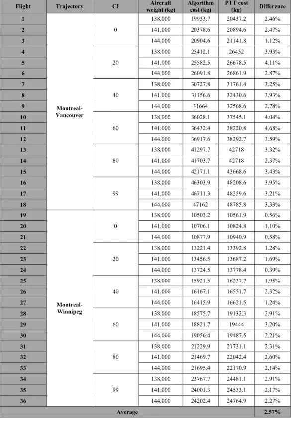
All flight phases are considered in order to obtain the best possible optimization results. The new algorithm improves the path planning and reduces flight cost. Additional altitude, speed and time restrictions are also considered in the development of this optimization algorithm. The new algorithm was developed in Matlab® based on the PDB for different commercial aircraft, and it is capable of reducing the fuel burn with an average of 2.57% (to the date).
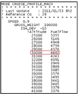
Fundamental research data for this project is given by the PDB. The numerical model of the aircraft provides all the necessary information to create the algorithm. The PDB is a database of approximately 30,000 lines, which gives the information about real aircraft performances. It indicates the fuel consumption and the distance flown for a specific flight profile (climb, cruise or descent). For example, the fuel burn and distance for an aircraft cruising with a center of gravity of 28% of the mean aerodynamic chord, flying at 0.8 Mach with a total gross weight of 100 tons, at an altitude of 30,000 ft and a standard deviation temperature of -10ºC. Such an example is shown on Figure 3.1:
Figure 3.1 Example of information given on the PDB
The PDBs includes as inputs the aircraft weight, altitude, speed, center of gravity and air temperature, and the outputs are the traveled distance and the fuel burn. The traveled time is calculated from the aircraft’s TAS, while the wind influence is calculated with a wind triangle methodology, providing a traveled distance correction factor depending on the wind angle and speed. The wind speed and direction are entered manually into the algorithm, at four different altitudes, at each flight WP, in the same way as on the FMS.
The PDB contains very detailed aircraft information; however, there are five main tables that are used in this program and can be observed in Table 3.1.
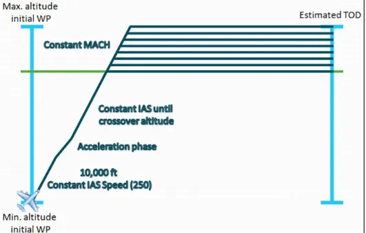
The wind influence on the trajectory will be calculated using the wind triangle method (Figure 3.2). As the aircraft flights on a straight path, the wind affects the aircraft’s speed. Depending on the direction and speed of the wind, the distance traveled by the aircraft will be either reduced or augmented in a time segment.
31
Table 3.1 Inputs and outputs for the PDB for a commercial aircraft
Type of table Inputs Outputs
Climb Center of gravity
Speed Gross weight ISA deviation Altitude Fuel burn Horizontal distance
Climb acceleration Gross weight Initial Speed Initial Altitude Delta speed Fuel burn Horizontal distance Delta altitude Cruise Speed Gross weight ISA deviation Altitude Fuel flow
Descent deceleration Vertical speed Gross weight Initial speed Final altitude Delta speed Fuel burn Horizontal distance Delta altitude Descent Speed Gross weight Standard deviation Altitude Fuel burn Horizontal distance
The wind factor can be calculated in the following way (Langlet, 2011): ) cos( * || || || || || || || || )* sin( arcsin cos _ θ θ speed speed speed speed Air Wind Air Wind factor Wind − = (3.6) 3.4 Climb
The PDB divides the TAS values in two different types of speeds: IAS (Indicated AirSpeed) and Mach number. The TAS varies with the altitude. For the IAS case, the TAS increases with the altitude, while Mach decreases with the altitude. The altitude for which the TAS due to IAS is equal to the TAS due to Mach is called the crossover altitude. Table 3.2 represents an example for a 300/0.82 speed schedule (composed from an IAS/Mach pair), with an altitude step of 1,000 ft.
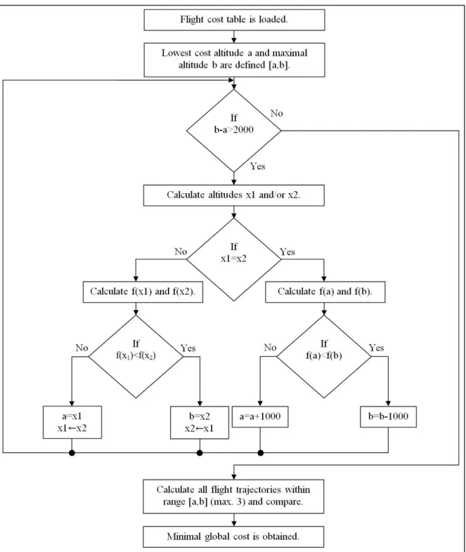
The climb phase consists of four different phases:
• Initial climb. Aircraft is located initially at 2,000 ft, and will climb up to 10,000 ft at a constant predefined speed (normally 250 IAS).
• Acceleration phase. Aircraft will accelerate to the selected optimal IAS speed.
• IAS climb. Aircraft will climb at a constant IAS speed after the acceleration phase until the crossover altitude.
• Mach climb. Once the aircraft reaches the crossover altitude, it will climb at a constant Mach speed.
For the purpose of this project and in order to reduce processing time, the Mach speed selected during the cruise phase remains constant through the complete flight. Speed variation during the cruise phase will be considered for future work.
To select the optimal climb for the flight, all available speed schedules will be calculated. Each speed schedule expressed as IAS/Mach has its own crossover altitude that can be seen in Table 3.3. For each IAS/Mach couple, the crossover altitude is calculated using a 1,000 ft altitude step.
33
Table 3.2 Crossover altitude example for a 300/0.82 speed schedule Altitude (ft)
TAS due to an IAS of 300 knots
(knots)
TAS due to a Mach number of 0.82 (knots) 10,000 345.4 523.2 11,000 350.4 521.3 12,000 355.6 519.4 13,000 360.8 517.4 14,000 366.1 515.5 15,000 371.6 513.5 16,000 377.1 511.6 17,000 382.7 509.6 18,000 388.4 507.7 19,000 394.3 505.8 20,000 400.2 503.8 21,000 406.3 501.4 22,000 412.5 499.4 23,000 418.8 497.5 24,000 425.2 495.6 25,000 431.7 493.6 26,000 438.3 491.2 27,000 445.1 489.2 28,000 452.0 487.3 29,000 459.0 485.4 30,000 466.2 482.9 31,000 473.4 481.0 32,000 480.8 479.0 33,000 488.4 476.6 34,000 496.1 474.7 35,000 503.9 472.7 36,000 512.5 470.3 37,000 521.8 470.3 38,000 531.6 470.3 39,000 542.0 470.3
The aircraft climbs at a constant 250 IAS from 2,000 ft to 10,000 ft. At 10,000 ft, the acceleration tables are created for each IAS speed. At the final acceleration altitude, the climb for each available IAS is calculated up to the maximal climb altitude (normally, 40,000 ft). The aircraft will only cruise at the Mach speed. After the IAS climb table is calculated, the Mach climb is calculated from the crossover altitude and up to the maximal altitude.
From the crossover altitude and for each 1,000 ft over the crossover altitude, the cruise cost is calculated for the entire length of the flight and is saved in the flight cost table. The flight cost table contains all the possible speed schedules and all the possible cruise altitudes. From the minimal cruise altitude (20,000 ft) to the maximal altitude, only the lowest cost speed schedule for each altitude is selected. Figure 3.3 represents the climb phase.
Table 3.3 Crossover altitudes table (ft)
IAS/ Mach 250 260 270 280 290 300 310 320 330 340 350 360 0.78 38,000 36,000 35,000 33,000 31,000 30,000 28,000 27,000 25,000 24,000 22,000 21,000 0.785 38,000 36,000 35,000 33,000 32,000 30,000 29,000 27,000 26,000 24,000 23,000 21,000 0.79 39,000 37,000 35,000 34,000 32,000 30,000 29,000 27,000 26,000 24,000 23,000 22,000 0.795 39,000 37,000 35,000 34,000 32,000 31,000 29,000 28,000 26,000 25,000 23,000 22,000 0.8 39,000 37,000 36,000 34,000 33,000 31,000 30,000 28,000 27,000 25,000 24,000 22,000 0.805 39,000 38,000 36,000 34,000 33,000 31,000 30,000 28,000 27,000 25,000 24,000 23,000 0.81 39,000 38,000 36,000 35,000 33,000 32,000 30,000 29,000 27,000 26,000 24,000 23,000 0.815 40,000 38,000 37,000 35,000 34,000 32,000 30,000 29,000 28,000 26,000 25,000 23,000 0.82 40,000 39,000 37,000 35,000 34,000 32,000 31,000 29,000 28,000 26,000 25,000 24,000 0.825 40,000 39,000 37,000 36,000 34,000 33,000 31,000 30,000 28,000 27,000 25,000 24,000 0.83 40,000 39,000 38,000 36,000 34,000 33,000 31,000 30,000 29,000 27,000 26,000 24,000 0.835 41,000 39,000 38,000 36,000 35,000 33,000 32,000 30,000 29,000 27,000 26,000 25,000 0.84 41,000 39,000 38,000 36,000 35,000 33,000 32,000 31,000 29,000 28,000 26,000 25,000
35
3.5 Cruise
The cost optimization algorithm calculates the optimal trajectory depending on the flight length. For short flights (under 500 nm), where usually flight restrictions are not changed during the flight, the algorithm obtains the lowest cost altitude and speed schedule from the flight cost table. For short flights, the descent phase has high influence on the global cost of the flight. Since the descent is the lowest cost phase during a flight, it is possible that would be better if the aircraft would climb higher (higher cost) in order to have a longer descent and a shorter cruise. The cost optimization algorithm uses the Golden Section search optimization algorithm for the cruise. Calculating all the possible descents for the flight cost table would result in an excessive (and unnecessary) calculation time, therefore, the Golden Section method is applied. The Golden Section method is a non linear optimization method that reduces the search interval by the same fraction, with each iteration, at a golden section ratio, which is commonly known in mathematics as the golden ratio (Venkataraman, 2009). The golden section search was selected over other interval reducing methods, such as the dichotomous search or the Fibonacci method, because its efficiency and ease of implementation. The dichotomous search calculates two new evaluations at each iteration, while the golden section search and the Fibonacci method only calculate one new evaluation at each new iteration. The Fibonacci method, however, reduces the size of the interval by the Fibonacci series, which changes the reduction size with each iteration. The golden section search uses a fixed interval reduction, making it simpler to implement.
Applied to the trajectory optimization algorithm, the Golden Section search is the most adequate of the interval reducing methods. The fewest number of iterations are obtained, and its simplicity reduces the algorithm processing time.
The algorithm obtains the lowest cost speed schedule and altitude, which may not be the maximal altitude. Since it could be possible that climbing at a higher altitude (to have a longer descent phase) would result in a lowest global cost trajectory, the method should calculate the descent for all possible altitudes over the cost altitude selected from the flight