Direct numerical simulation of unsheared turbulence diffusing toward a free-slip or no-slip surface

O

pen

A

rchive

T

oulouse

A

rchive

O

uverte (

OATAO

)

OATAO is an open access repository that collects the work of Toulouse researchers

and makes it freely available over the web where possible.

This is an author -deposited version published in:

http://oatao.univ-toulouse.fr/

Eprints ID: 4166

To link to this article: DOI: 10.1080/14685248.2010.521632

URL:

http://dx.doi.org/10.1080/14685248.2010.521632

To cite this version: BODART Julien, CAZALBOU Jean-Bernard, JOLY Laurent.

Direct numerical simulation of unsheared turbulence diffusing toward a free-slip or

no-slip surface. Journal of Turbulence, 2010, vol. 11, n° 48.

ISSN 1468-5248

Any correspondence concerning this service should be sent to the repository administrator:

Direct numerical simulation of unsheared turbulence diffusing toward a free-slip or no-slip surface

J. BODART, J.-B. CAZALBOU and L. JOLY Universit´e de Toulouse, ISAE

BP 54032, 31055 Toulouse cedex 04, France

(Received 00 Month 200x; final version received 00 Month 200x)

The physics involved in the interaction between statistically steady, shearless turbulence and a blocking surface is investigated with the aid of direct numerical simulation. The original configuration introduced by Campagne et al. [1] serves as the basis for comparing cases in which the blocking surface can be either a free-slip surface or a no-slip wall. It is shown that in both cases, the evolutions of the anisotropy state are the same throughout the surface-influenced layer (down to the surface), despite the essentially different natures of the inner layers. The extent of the blocking effect can thereby be measured through a local (surface) quantity identically defined in the two cases. Examination of the evolution and content of the pressure-strain correlation brings information on the mechanisms by which energy is exchanged between the normal and tangential directions : In agreement with an earlier analysis by Perot and Moin [2], it appears that the level of the pressure-strain correlation is governed by a splat/antisplat disequilibrium which is larger in the case of the solid wall due to viscous effects. However, in contradiction with the latter, the pressure-strain correlation remains as a significant contributor to both Reynolds-stress budgets; it is argued that the net level of the splat/antisplat disequilibrium is set, in the first place, by the normal-velocity skewness of the interacting turbulent field. The influence of viscous friction on the intercomponent energy transfer at the solid wall only comes in the second place and part of it can also be measured by the skewness. The remainder seems to originate from interactions between the strain field and ring-like vortices in the vicinity of the splats.

Keywords: Wall-bounded turbulence; Direct numerical simulation; Intercomponent energy transfer; Blockage effect; Reynolds-stress budgets.

1. Introduction

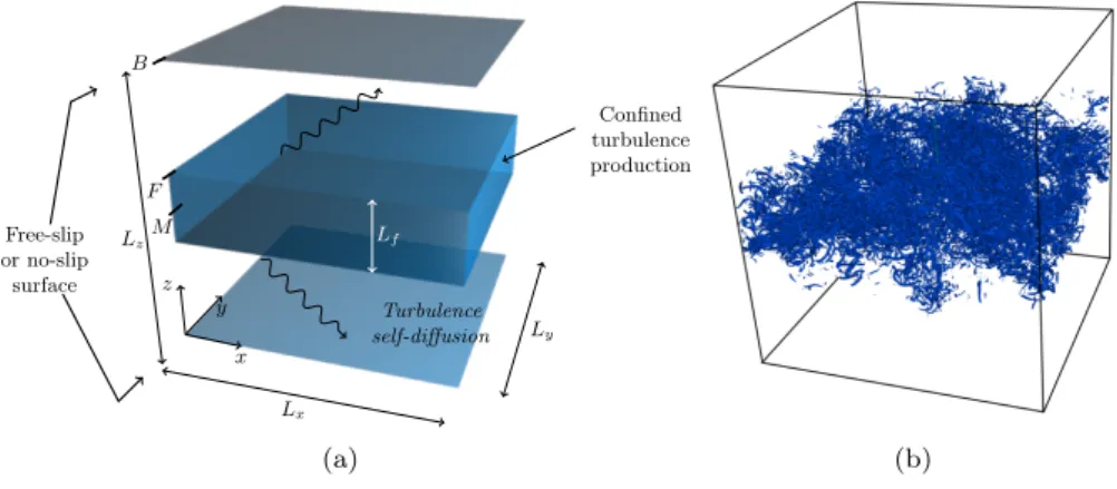
We consider the original flow configuration designed by Campagne et al. [1] to study the interaction between statistically steady, unsheared turbulence and a blocking surface by means of direct numerical simulation (DNS). In this configuration, the flow develops inside a cubic domain where turbulence production by a random force field is confined inside a thin layer of fluid located at the same distance from two opposite faces of the cube (see figure 1). Depending on the nature of the boundary conditions imposed at these faces, two kinds of blocking surfaces can be considered: rigid free-slip surfaces or no-slip solid walls. After a transient, a statistically steady state is obtained in which turbulence experiences a spatial decrease across a pure-diffusion region located between the turbulence-production layer and the considered surface. In the work of Campagne et al. [1], the simulation was performed with a fully pseudo-spectral Fourier solver and, due to the inherent limitations of this type of numerical approach, the study had to be limited to the case of a free-slip surface. In order to overcome such a limitation, a new solver has been built using a mixed spectral/finite-difference discretization. It allows a direct

Confined turbulence production Turbulence self-diffusion z y x Lf Ly Lx Lz F B M Free-slip or no-slip surface (a) (b)

Figure 1. Sketch of the flow configuration (a) and general idea of the flow field (b). Capital letters in (a) refer to remarkable (x, y) planes: B, blocking surface; F, edge of the turbulence-production region; M, midplane. Contour surfaces in (b) correspond to isovalues of the second invariant of the velocity-gradient tensor (Q-criterion) and outline the vortical activity present in the flow field.

comparison of the free-surface and solid-wall cases (hereafter referred to as FS and SW) computed with strictly identical forcing fields, fluid properties (density, viscosity), and domain dimensions/discretization. Our purpose is therefore twofold: first, to fully document both variants of the flow and, second, to step-by-step understand the physics involved in the intercomponent energy transfer mechanism near a blocking surface.

As regards the first point, our flow configuration can be viewed as the numerical analog of an oscillating-grid experiment with a plane blocking surface located at some distance from the grid. Since the initial work of Rouse and Dodu [3], the use of oscillating grids has been widely adopted to perform experiments in which a statistically-steady turbulent flow has to be maintained without resorting to tur-bulent production by mean shear. Among the wealth of problems investigated that way, the interaction with a plane boundary has been little considered: Brumley and co-workers [4, 5] have performed an experiment on the interaction between oscillating-grid turbulence and a gas-liquid interface which is a good representa-tion of an ideal free-surface when the Froude number is low. The case of a solid wall has been marginally documented by McDougall [6] and Hannoun et al. [7] for comparison with more extensive investigations of the interaction with a sharp density interface.

Turning now to the question of the intercomponent energy transfer, it is now well established that, while the pressure-strain correlation behaves usually as a return-to-isotropy mechanism, the picture changes drastically in the vicinity of the surface where it promotes energy transfer from the normal toward the tangential directions, i.e. from the less energetic toward the most energetic normal stress. This is observed in free-surface flows as well as in wall-bounded flows. Such be-haviour has long been attributed to the “splat” effect (see for instance Bradshaw and Koh [8]): due to kinematic blocking, packets of fluid impacting the surface transfer their normal kinetic energy to directions parallel to the surface. This in-terpretation has later been extended by Perot and Moin [2] to take into account the necessary counterpart of the splat mechanism: the “antisplat” mechanism by which collisions between packets of fluid travelling along the surface produce ejec-tions of fluid in the normal direction. The two sides of the splat/antisplat process lead to opposite contributions to the pressure-strain correlation and, consistently, Perot and Moin have suggested that the net level of the correlation should be de-termined by the imbalance between the two kinds of events. In their comparative study of initially-isotropic turbulence decaying in the presence of either a free

sur-3

face or a solid wall, they further concluded that the imbalance should be basically attributed to the action of viscosity. This statement was later mitigated by Walker et al.in a study of the same flow configuration performed at larger times. At these later stages, anisotropy had become significant, and comparing their results with those obtained at shorter times by Perot and Moin, Walker et al. concluded that the local level of stress anisotropy should also control the amount of intercompo-nent energy transfer. Walker et al. also pointed out that, in this time-decaying flow, the decay rates of the normal and tangential components of the fluctuation are significantly different and that the latter is nonuniform across the flow. Thus, anisotropy is not controlled, neither in time nor space. We shall see that, in our configuration, statistical steadiness helps to keep a reference anisotropy level in the far field and yields Reynolds-stress budgets that are not dominated by dissipation and time-variation terms. Moreover, the structure of the flow is closer to a tra-ditional turbulent boundary-layer arrangement with turbulence being essentially produced at some distance from the wall. It will become apparent that these char-acteristics help to get a better insight into the physical processes that set the level of the pressure-strain correlation in wall-bounded turbulence.

2. Numerical details

The incompressible Navier-Stokes equations are solved in a hybrid Fourier/physical space. A pseudo-spectral Fourier algorithm is used in the directions parallel to the surface (x and y) with periodic boundary conditions, while a sixth-order com-pact scheme (Lele [9]) is retained to discretize the differential operators along the surface-normal direction (z). Time discretization of the momentum equation is based on a third-order Runge-Kutta scheme for the advective terms and a second-order Crank-Nicholson scheme for the viscous terms. A predictor-corrector method similar to that of Lamballais [10] is used to enforce continuity. The dimensions of the domain (Lx, Ly, Lz) and numerical grids are the same in the FS and SW cases. The dimensions of the domain are all taken equal to 6, and the numerical grid involves 512 dealiased modes in the x and y directions with 512 points in the surface-normal direction. A cosine mapping in the latter direction is used to ensure full spatial resolution in the near-surface region.

We use the turbulence-production mechanism proposed by Bodart et al. [11]. It is based on the use of a random force field f (x, t) implemented as a source term at the right-hand side of the Navier-Stokes equations:

∂ui ∂t + uj ∂ui ∂xj = −1 ρ ∂P ∂xi + ν ∂ 2_u i ∂xj∂xj + fi(x, t).

The force field is required to be (i) divergence-free so as to avoid any spurious influence on the pressure field, (ii) time decorrelated, and (iii) confined inside a production layer which is located halfway between the two blocking surfaces and the thickness of which is chosen as Lf = 2. In order to meet the above requirements, the construction of f (x, t) relies on spatial arrangements of several cubic “forcing boxes” of size lf < Lf in which three kinds of elementary force fields e(x) can be implemented in the form

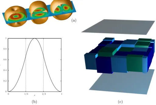
eα(x) = φ(xα) φ0(xβ) φ(xγ), eβ(x) = −φ0(xα) φ(xβ) φ(xγ) and eγ(x) = 0, where (α, β, γ) corresponds to any of the three direct permutations of the indices (1, 2, 3) [see figure 2(a)] , and φ(x) is chosen as a second-order spline function

x φ 1 2/3 1/3 0 1 0.8 0.6 0.4 0.2 0 (b) (c) (a)

Figure 2. Turbulence-generation method. (a) Isosurfaces of the force modulus in the three types of ele-mentary force fields e(x); (b) plot of the forcing function φ(x); (c) typical arrangement of the forcing boxes at a given time step, each colour refers to a different type of elementary force field.

Table 1. Flow parameters obtained in the remarkable (x, y) planes referenced in figure 1.

The definition of the Taylor-microscale Reynolds number Reλ is based on the horizontal

rms velocity fluctuation u0and longitudinal microscale λx

x, that of the turbulent Reynolds

numbers Rel on the square root of the turbulent kinetic energy k and turbulent length

scale ` = k3/2/ε (ε is the turbulent dissipation rate). The reference value for viscosity is

ν = 1/1200.

Free-slip surface No-slip wall Location z/L `/L Reλ Rel z/L `/L Reλ Rel

M (z = Lz/2) 16.4 10.4 329 3453 16.4 10.5 327 3435

F (z = Lz/3) 10.9 3.0 103 367 11.0 2.9 100 337

B (z = 0) 0 11.9 79 358 0 0 0 0

defined on the interval [0, lf = 1.5] that goes to zero with a zero derivative at either ends of the interval [see figure 2(b).] At each time step, a different arrangement of 4 × 4 elementary force fields of the three kinds is implemented in the production layer with random individual shifts in the z direction and a random global shift in the x and y directions (see a typical arrangement in figure 2(c).) The specific arrangement and values of the shifts are randomly renewed at each time step in order to ensure time decorrelation, the shifts along z are limited so that the forcing boxes always remain inside the production layer. Table 1 summarizes the values of the flow parameters that result from the implementation of the forcing method. In particular, the values of the length scales and Reynolds numbers at the edge of the production layer precisely define the flow configurations under study.

The statistical treatment performed on the results makes the best possible use of the geometrical properties of the flow configuration: statistical homogeneity along the x and y directions, symmetry with respect to the midplane and rotational symmetry about the z axis. Statistical steadiness allows the data to be further averaged in time: 3000 instantaneous fields are gathered during a time sample that amounts to 22 T∗, where the turbulent time scale T∗ is defined as the maximum value in the domain of the ratio between the turbulent kinetic energy (k) and dissipation rate (ε). Total computations required about 50,000 CPU hours for each case on an IBM/POWER6 platform.

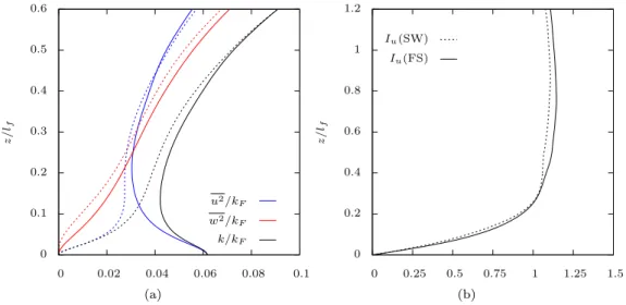
0 0.1 0.2 0.3 0.4 0.5 0.6 0 0.02 0.04 0.06 0.08 0.1 z / lf u2_/kF w2_/kF k/kF (a) 0 0.2 0.4 0.6 0.8 1 1.2 0 0.25 0.5 0.75 1 1.25 1.5 z / lf Iu(SW) Iu(FS) (b)

Figure 3. Profiles of (a) the Reynolds stresses and turbulent kinetic energy across the flow, and (b) of the corresponding isotropy factor Iu= w0/u0. The vertical coordinate z is normalized with the characteristic

scale lf of the turbulent-production process, and the Reynolds stresses with the value kF of the turbulent

kinetic energy at the edge of the turbulence-production region. Solid lines refer to the FS case and dashed lines to the SW case.

3. Flow structure

Starting from the turbulence-production layer and as the surface is approached, the flow structure involves several distinct regions: First, a pure-diffusion region in which turbulence is self-transported toward the surface. Second, further away from the turbulence-production region, the flow enters a surface-influenced layer, which is subject to (i) the kinematic (impermeability) condition, and (ii) the dynamic (free-slip or no-slip) boundary condition. The influence of the kinematic condition is felt farther from the surface than that of the dynamic boundary condition. For this reason, the surface-influenced layer can be denoted as the outer “blockage” layer. It includes, adjacent to the surface, an inner layer that will be denoted as the “slip” or “viscous” layer depending on the precise nature of the dynamic boundary condition.

In the pure-diffusion region, the flow structure is governed by a balance between turbulent diffusion and dissipation. This situation is encountered in oscillating-grid experiments for which the length scale increases linearly with the distance to the turbulent source while the turbulent kinetic energy decreases (see for instance Hopfinger and Toly [12]). According to the body of experimental results, the isotropy factor Iu (defined as the ratio between the rms values of the vertical and horizontal velocity fluctuations: w0_/u0_{) remains constant in this region, in the range} 1.1–1.3. The influence of the impermeability condition, according to which the surface-normal velocity component cancels at the surface, can obviously be traced through the evolution of the velocity isotropy factor. Thus, the blockage layer will be defined as the region across which it goes from its value in the pure-diffusion region down to zero at the surface. Figures 3(a) and 3(b) show, respectively, the vertical evolutions of the Reynolds stresses and the corresponding evolutions of the isotropy factors in the two flow configurations. The plots of the Reynolds-stress are in agreement with the surface asymptotics in both cases, that is: u2 _{∝ 1} and w2 _{∝ y}2 _{in the FS case; u}2 _{∝ y}2 _{and w}2 _{∝ y}4 _{in the SW case. As a result,} the isotropy factors go to zero as y at the surface in either case. The most striking feature however is the very similar profiles obtained in the two cases and, more specifically, the very close values obtained for the slopes of Iu at the surface. Such similarity confirms an implication of the high-Reynolds-number theory of Hunt and

Graham [13] according to which the blocking effect in the outer layer should not depend on the precise nature of the dynamic boundary condition. The close values obtained for the slopes at the surface further indicate that the same holds in the inner layers despite their essentially-different natures. Such a result prompts one to generalize to the case of the solid wall the suggestion of Campagne et al. [14] to use the length scale L = ( dIu/dz|z=0)

−1

as a measure of the blockage-layer thickness. The values obtained for L in the FS and SW cases amount to 0.122 lf and 0.121 lf, respectively. Considering in figure 3(b) that the isotropy factors depart from their “pure-diffusion” values (≈ 1.1 here) at z ≈ 0.6 lf, the actual thickness of the outer blockage layer appears as being about 5L, which is consistent with the range given by Campagne et al. [14].

Concerning the inner layers, an essential difference between the two dynamic boundary conditions arises from their consequences on the vortex dynamics near the surface: the free-slip condition yields a vorticity vector normal to the surface while the no-slip condition imposes that it becomes tangential. This difference is apparent in figure 4(a), where the variances of the horizontal (ω2

x) and vertical (ωz2) vorticity components have been plotted across the flow. A vorticity isotropy factor Iω can then be defined as the square root of the ratio ωx2/ω2z. Its evolution is plot-ted in figure 4(b) for the two cases and stresses the differences in the inner-layer behaviours. Across the pure-diffusion region, the value Iω remains fairly constant, slightly above unity. Then, proceeding toward the surface, the value of Iω rises significantly while getting close to the surface in the upper part of the outer layer. Vorticity profiles obtained by Leighton et al. [15] for the free surface of an open-channel flow or Shen et al. [16] for the interaction between a time-evolving wake and a free-surface indicate a similar behaviour for Iω. The enstrophy budgets pre-sented in the same references show that the rise of the isotropy factor toward the surface is a blockage-layer effect due to the prevalence of vortex stretching along the tangential direction in this region. Entering the inner layers, the evolutions of Iω finally diverge: they exhibit a steep return to zero in the FS case and keep in-creasing up to infinity in the SW case, consistently with each boundary condition. Following Campagne et al. [14], the thickness δsof the slip layer in the FS case will be defined as the distance to the surface at which Iω reaches its maximum, here we find δs = 0.035 lf. In the SW case, a consistent definition of the thickness of the viscous layer (δv) will need an examination of the kinetic-energy budget, and cannot be given at this stage.

4. Reynolds stresses budgets

In this configuration, the flow is statistically steady, invariant under rotation about the z axis and homogeneous along the x and y directions. The Reynolds stress ten-sor is therefore diagonal and all the statistical information at this level is contained in the variances of the vertical component (w) and any horizontal component (u or v) of the velocity fluctuation. The budget equations for the nonzero Reynolds

7 0 0.1 0.2 0.3 0.4 0.5 0.6 0 0.005 0.01 0.015 0.02 0.025 0.03 z / lf ω2 x/ω2F ω2 z/ω2F ω2_/ω2_F (a) 0 0.2 0.4 0.6 0.8 1 1.2 0 0.5 1 1.5 2 2.5 z / lf Iω(SW) Iω(FS) (b)

Figure 4. Profiles of (a) the variances of the vorticity components and enstrophy [ω2_{= (ω}2

x+ ω2y+ ω2)/2],

and (b) of the corresponding isotropy factor Iω = ωx0/ω0z. The vertical coordinate z is normalized with

the characteristic scale lf of the turbulent-production process, and the vorticity variances with the value

ω2

F of the enstrophy at the edge of the turbulence-production region. Solid lines refer to the FS case and

dashed lines to the SW case.

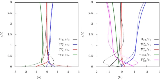
stresses then reduce to: 0 = −∂u 2_w ∂z | {z } Du 11 + ν∂ 2_u2 ∂z2 | {z } Dν 11 +2 ρp ∂u ∂x | {z } Π11 − 2ν ∂u ∂xk ∂u ∂xk | {z } ε11 , (1) 0 = −∂w 3 ∂z | {z } Du 33 + ν∂ 2_w2 ∂z2 | {z } Dν 33 +2 ρp ∂w ∂z | {z } Π33 −2 ρ ∂pw ∂z | {z } Dp 33 − 2ν∂w ∂xk ∂w ∂xk | {z } ε33 , (2) where Du ij, D p

ij, Dνij and εij denote, respectively: turbulent diffusion by velocity fluctuations, by pressure fluctuations, viscous diffusion and the dissipation-rate tensor. Figures 5(b) and 5(a) display the budgets of the nonzero Reynolds stresses u2 _{and w}2 _{as functions of the normal distance to the surface. In the FS case, the} budgets are remarkably consistent with those obtained by Campagne et al. [1], and also with those obtained in free-surface channel flows (see for instance Handler et al. [17]). Far from the surface, the magnitudes of the different terms are very similar to those found in the SW case. However, we get a clear contrast in the inner layers, in response to the slip or no-slip boundary condition: In the budget of the horizontal component, viscous diffusion balances dissipation in the SW case while both of them act in the same way and balance turbulent diffusion in the FS case. In the former case the budget can be considered as fully dominated by the viscous effects up to z ≈ 0.15L which gives a measure of the viscous-layer thickness. The pressure-strain correlation plays a similar role in both cases. In the near-surface region it is a sink term for the normal stress and a source term for the tangential stress. This expected feature was already described by Walker et al. [18] and Perot and Moin [2]. In contrast with the standard return-to-isotropy effect embedded in the pressure-strain correlation remote from walls, the intercomponent energy transfer is thus reversed and produces anisotropy in the near-surface region. The interpretation given by Perot and Moin [2] refers to the splat and antisplat mechanisms according to which energy is removed from the normal component and transferred the tangential one (splat) and, conversely, from the tangential to the

0 0.5 1 1.5 2 2.5 3 -3 -2 -1 0 1 2 3 z /L Π11/εc Du 11/εc Dν 11/εc −ε11/εc (a) 0 0.5 1 1.5 2 2.5 3 -2 -1 0 1 2 3 z /L Π33/εc Du 33/εc Dν 33/εc −ε33/εc Dp 33/εc (b)

Figure 5. Reynolds-stress budgets across the flow. (a) u2_{; (b) w}2_{. All terms have been arbitrarily}

normal-ized by εcthe value of the dissipation rate at z/L = 3 (top of the graph) in order to ease the comparison

between the FS case (solid lines) and the SW case (dashed lines).

normal component (antisplat). It was further claimed that viscous friction along the wall prevents the total amount of kinetic energy transferred to the tangential component by the splat events, from being restored to the normal component by the antisplat events. In our simulations, it appears that viscous friction only yields a minor increase in the magnitude of Π33in the SW case as compared to the FS case. Interestingly, the pressure-strain is a significant contributor to both budgets and keeps the same order of magnitude in the two cases. This suggests that another reason than the effect of viscosity has to be found to explain the wealth of the splat/antisplat imbalance.

5. Intercomponent energy transfer

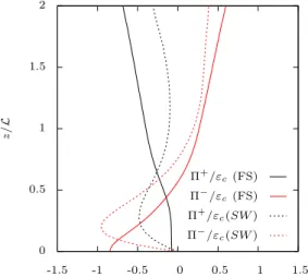
The splat/antisplat mechanism refers to impacts/ejections of fluid along the normal direction. It can be traced in instantaneous fields by following the sign of the normal velocity component. Moreover, due to the vanishing of the normal velocity at the surface in both cases, the behaviours of w and its normal derivative denoted as ∂zw are closely connected in the immediate neighbourhood of the surface. Splat events, associated to fluid packets moving toward the surface, involve negative values of the vertical strain rate ∂zw. Antisplat events, associated to fluid packets moving away from the surface yield positive ∂zw. Accordingly, we split the contributions to the normal pressure-strain correlation Π33 into two parts, Π+ and Π−, by applying a conditional sampling based on the sign of ∂zw. Figure 6 shows such a decomposition in the SW and FS cases. In both situations, the sign of the Π−_{correlation switches} to negative in the vicinity of the boundary, in agreement with the idea of splats driving normal kinetic energy from the normal to the tangential components. The Π+ _{correlation, almost vanishes at the free-slip surface and unexpectedly brings} an extra negative contribution to Π33 near the solid wall. This paradoxical result suggests that, in this case, the intercomponent transfer results from a more complex mechanism than the simple splat/antisplat disequilibrium put forward by Perot and Moin [2]. We shall now take a closer look to these elementary events and try to decipher how they contribute to the pressure-strain correlation.

9 0 0.5 1 1.5 2 -1.5 -1 -0.5 0 0.5 1 1.5 z /L Π+_/ε c(FS) Π−/εc(FS) Π+/εc(SW ) Π−/εc(SW )

Figure 6. Pressure-strain split according to the sign of ∂zw. All terms are normalized by εc(see figure 5).

5.1. Quadrant decomposition

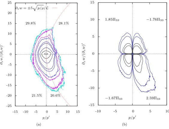
In order to understand how local events can build up the pressure-strain correlation, we unfold its content in the (p, ∂zw) plane at a given distance from the surface. Figures 7 and 8 show the results of this analysis. For each case, isocontours of the pressure/strain-rate joint probability density function and contribution to Π33 are given at the reference height z0. This reference corresponds to the value of z at which the pressure-strain correlation reaches its maximum near the surface. It is thus strictly equal to zero in the FS case and has been found equal to 0.21 L in the SW case. Selecting these values ensures that the pressure-strain correlation is of the same order of magnitude in both cases. The step between two running contours follows a logarithmic progression in order to maximize the number of visible contours. In these plots, splat and antisplat events are expected to lie in the lower-right and upper-right quadrants, respectively. They can be more precisely localized considering that, when a fluid packet of size l meets the surface with a velocity of order w, the corresponding pressure rise and vertical strain rate can be estimated as p/ρ ≈ w2_{/2 and ∂}

zw ≈ w/l. Then, the vertical strain-rate fluctuation can be written as a function of the pressure fluctuation under the form ∂zw ≈ l−1

p

2p/ρ. A similar reasoning leads to the same form and an opposite sign for the strain-rate fluctuation corresponding to an antisplat event. In the (p, ∂zw) plane, these forms correspond to a family of parabolic curves on which the splat and antisplat events of different sizes l should focus. The curves obtained with particular sizes ls (corresponding to ls/L =

√

2/5 ≈ 0.3 in the FS case and √

2/3 ≈ 0.5 in the SW case) have been drawn in figures 7(a) and 8(a). These particular values have been eye-adjusted so that the curves match with the general shape of the contour pattern. If the variables were uncorrelated the pattern would be perfectly symmetrical with respect to both axis. Here, we see that it is bent over our particular parabolic curves. Interestingly, the corresponding values of l fall close to the distance from the surface over which most of the intercomponent energy transfer due to the blockage effect occurs (see the Reynolds-stress budgets in figure 5.) This seems to confirm the presence of both kinds of events in the FS case. Things are not so clear, however, in the SW case where two majors differences with the FS case can be noticed. The first one is the disappearance of the most energetic events (as regards the pressure fluctuation) in the upper-right quadrant (antisplats), together with a significant reduction in the cumulative contribution to Π33 from this quadrant: −0.42 Π33 while the contribution relative to the same quadrant in the FS case amounts to −1.76 Π33(see figures 7(b) and 8(b)). Following

-25 -20 -15 -10 -5 0 5 10 15 20 25 -15 -10 -5 0 5 10 15 ∂z w / (∂ z w ) ′ p/p′ 29.8% 28.1% 21.5% 20.6% ∂zw =±5 p p/ρ/L (a) -15 -10 -5 0 5 10 15 -10 -5 0 5 10 ∂z w / (∂ z w ) ′ p/p′ 1.85Π33 −1.76Π33 −1.67Π33 2.59Π33 (b)

Figure 7. Quadrant analysis of the pressure-strain correlation at z = 0 in the FS case: (a) isocontours of the pressure/strain-rate joint probability density function; (b) isocontours of the contribution to Π33.

The horizontal and vertical axis are normalized with the rms values p0 _{and (∂}

zw)0 of the pressure and

strain-rate, respectively. -25 -20 -15 -10 -5 0 5 10 15 20 25 -15 -10 -5 0 5 10 15 ∂z w / (∂ z w ) ′ p/p′ 33.9% 26.0% 18.9% 21.2% ∂zw =−3 p p/ρ/L (a) -15 -10 -5 0 5 10 15 -10 -5 0 5 10 ∂z w / (∂ z w ) ′ p/p′ 0.74Π33 −0.42Π33 −0.39Π33 1.07Π33 (b)

Figure 8. Quadrant analysis of the pressure-strain correlation at z = 0.21 L in the SW case: (a) isocontours of the pressure/strain-rate joint probability density function; (b) isocontours of the contribution to Π33.

The horizontal and vertical axis are normalized with the rms values p0 and (∂zw)0 of the pressure and

11 0 2 4 6 8 10 12 -0.25 -0.2 -0.15 -0.1 -0.05 0 0.05 0.1 z /L FS SW

Figure 9. Profiles of the pressure-strain correlation coefficient CΠ= Π33/[p0(∂zw)0].

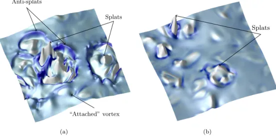
Perot and Moin, we can probably attribute this result to the viscous effects that slow down fluid packets moving along the wall before producing weak antisplats. The second difference with the FS case, that can be seen in comparing figures 7(b) and 8(b), comes from the rise in the cumulative contribution of the upper-left quadrant to Π33. It is apparent from its disequilibrium with the contributions of both the upper-right and lower-left quadrants (all three are roughly balanced in the FS case.) As regards the former, the disequilibrium leads to the negative sign of the conditional pressure-strain correlation Π+_{observed in figure 6 and part of it} can be explained at this stage by the disappearance of antisplats in the upper-right quadrant. The disequilibrium with the lower-left quadrant is harder to explain but cannot be neglected since it counts for 35% of the pressure-strain correlation (only 18% in the FS case), the remaining 65% coming from the disequilibrium between the right quadrants, i.e. the splat/antisplat imbalance (83% in the FS case). This point will be examined later but one can already notice that, the left quadrants corresponding to negative pressure fluctuations, rotational events are likely to be involved in this particular form of intercomponent energy transfer. Despite the aforementioned major differences, the contour plots obtained in the FS and SW cases exhibit some common characteristics in the lower-right (splat) quadrant that are worth to mention. First, the cumulative contribution from this quadrant is high: 2.59 Π33 in the FS case and 1.07 Π33 in the SW case. Second, the integrated probability of the corresponding events is small (20.6 % and 21.2 %, respectively) and the associated strain-rates are significantly larger than that observed in the other three quadrants. From this, it can be concluded that the energy transfer is driven at first order by a small number of high-intensity splat events. These are able to dominate a wealth of loosely correlated contributions for which the fluctuating pressure and strain rates are close to their rms values. The profiles of the pressure-strain correlation coefficient CΠ= Π33/[p0(∂zw)0] are given in figure 9 and confirm the picture drawn above. Its low value far from the surface shows that the pressure and strain-rate fluctuations are barely correlated there, while its increase close to the surface indicates the occurrence of correlated events. Figures 10(a) and 10(b) illustrate the aforementioned characteristics of the splat/antisplat events, using the field ∂zwto separate regions where the motion goes toward/from the surface. The strain-rate field (colour scale) is superimposed on a topographical representation of the pressure. The splat events appears as pressure peaks, they can be observed in the FS as well as SW cases. A striking feature in the FS case, and to a lesser extent in the SW case, is the presence of roughly circular pressure “valleys” surrounding

Anti-splats Splats “Attached” vortex (a) Splats (b)

Figure 10. Instantaneous maps of the strain-rate and pressure field, (a) at z = 0 in the FS case, and (b) at z = 0.21L in the SW case. The colour scale corresponds to the normal strain-rate field with contraction areas in white and extension areas in blue. The vertical ascending axis corresponds to the value of the pressure.

the splats, it will be shown further that they correspond to the rotational events hypothesized in the quadrant analysis. Also worth to notice is the very high intensity of the splats as compared to that of the antisplats: In order to satisfy the continuity equation, large areas of fluid slowly leaving the surface compensate for a few intense motions toward the surface.

5.2. Splat/anti-splat imbalance

In their numerical experiment, where the boundary condition is suddenly imposed at the edge of a cubic domain filled with decaying homogeneous turbulence, Perot and Moin [2] noticed that the amount of energy transfer was vanishingly small in the FS case but significant in the SW case. They suggest that the disequilibrium between splat/antisplat in the latter case is controlled by the viscosity which slows down the fluid packets moving along the wall before being ejected into the flow; while in the FS case, the absence of friction at the surface leads to a global equi-librium. In a similar simulation but at larger time, Walker et al. [18] introduced the idea that the return-to-isotropy mechanism was still present in the near surface region. It should act against the splat phenomenon, and therefore leave a signifi-cant amount of energy transfer at short time (low anisotropy level), and conversely inhibit the transfer at larger time (high anisotropy level). In our experiment, (i) the isotropy level is identical in both cases (see figure 3), and therefore the amount of energy transfer through the return-to-isotropy mechanism should be the same, (ii) the magnitude of the pressure-strain correlation is comparable in both cases, which suggests another reason than viscosity for the imbalance between splats and antisplats (iii) the imbalance appears as slightly higher in the SW case which does not rule out that viscosity still plays some role.

In order to find the reason for the imbalance between the two kinds of event, we shall try to evaluate the consequences of the dissymmetry observed above in the strain-rate distributions: small/large areas of fast/slow fluid moving toward/from the surface. The integrated probabilities in figure 7(a) help to quantify this dis-symmetry in the FS case: considering the percentage of realizations of events with a positive/negative normal strain rate, we can conclude to a large imbalance by 58% against 42%, in favor of the ejection events. The SW cases reveals an even

13

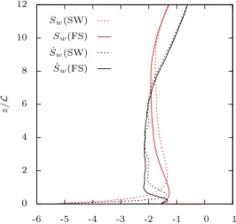
higher disequilibrium (60% against 40%). From a statistical point of view, the dis-symmetry of a fluctuating field can be measured by its skewness. Figure 11 shows the profiles obtained for this quantity when the normal velocity and strain rate are considered (Sw and ˙Sw, respectively). Both profiles are seen to be significantly negative all across the flow, which is consistent with our previous observations. This is also a well known feature of self-diffusing turbulence. For instance, in the shearless-turbulence mixing layer, experiments by Veeravalli and Warhaft [19] as well as simulations by Tordella et al. [20] indicate that high (absolute) values of Sw can be reached: 2.5 and 2.2 respectively, as compared to a maximum about 2 in our flow. The negative sign follows from the fact that the skewness is closely connected to the turbulent-diffusion flux w3 _{which is directed toward the surface (negative} with our orientation convention). Now, some basic physical considerations are nec-essary to understand how such a dissymmetry can lead to a significant imbalance in the contribution of the splat/antisplat process to the pressure-strain correlation. To this end, we resume our order-of-magnitude analysis according to which the splat/antisplat events can be locally assimilated to stagnation-point flows in which the (positive) pressure fluctuation p and the velocity fluctuation w at some distance lfrom the surface are correlated in the form p/ρ ≈ w2_{/2. It follows that the product} p/ρ × ∂zw can be approximated by w3/(2l) whatever kind of event is considered. Considering all the splat and antisplat events present in the flow, the global con-tribution to the intercomponent energy transfer should then have the same sign as and scale with w3_/l

s (recall that ls is a typical size of the fluid packets involved in the splat/antisplat process.) A direct connection is thus made between the level of the pressure-strain correlation Π33 and the skewness Sw = w3/w03. Such a con-nection has already been put forward by Magnaudet [21] who suggests that, in the limit of a weak far-field inhomogeneity (as compared to that imposed by the surface), the pressure-strain correlation should behave as Π33 = −2ε∞(2/3 + Sw). His conclusion is therefore opposite to ours since it entails that the pressure-strain correlation should decrease with Sw and eventually become positive below the crit-ical value Sw = −2/3. The idea of such a critical value is contradicted by our data showing that significantly negative pressure-strain correlations can be ob-tained together with values of Sw as low as −2. The reason is probably that the approach of Magnaudet is too restrictive to account for our flow configuration. It is based on an evaluation of the pressure-strain correlation obtained as the difference between modelled forms of the dissipation and turbulent-diffusion terms in a sim-plified Reynolds-stress budget. The dissipation and turbulent diffusion terms are then assumed to be constant across the ‘source’ layer, which may only be justified in the limit of a weak far-field inhomogeneity, and is clearly violated in our con-figuration (the deviation of our data to constant-value approximations are larger than the magnitude of the pressure-strain correlation itself.) By construction, the result cannot either be extended to situations where the skewness becomes very small (those of Perot and Moin [2] or Walker et al. [18] for instance), due to the central role of the turbulent-diffusion model in its derivation.

We shall therefore retain that, more generally, the contribution of the splat/antisplat imbalance to the pressure-strain correlation in the immediate vicin-ity of the surface (at the surface in the FS case and slightly above in the SW case) is essentially governed by the value of the skewness of the vertical fluctuation at some distance z = ls. The corresponding intercomponent energy transfer flows from the normal to tangential directions and its magnitude increases with the absolute value of the skewness. The distance ls is the typical size of the fluid packets involved in the splat/antisplat process and has been found to be about 0.3 ∼ 0.5 L in our analysis of the quadrant decompositions.

0 2 4 6 8 10 12 -6 -5 -4 -3 -2 -1 0 1 z /L Sw(SW) Sw(FS) ˙ Sw(SW) ˙ Sw(FS)

Figure 11. Profiles of the skewness Swof the vertical velocity component, and ˙Swof the vertical

strain-rate.

The role of viscosity, as suggested by Perot and Moin [2], is not in contradiction with the above statement: Figure 11 shows that the absolute value of the skew-ness increases in the vicinity of the surface when the latter is a solid wall. This observation simply reflects the fact that, viscous friction damping the tangential motions in the SW case, the antisplats become scarce thus eroding the positive tail of the normal-velocity probability-density function. This effect is marginal in our flow configuration where the reference value of the skewness is high due to the structure of self-diffusing turbulence. Accordingly, the net level of intercomponent energy transfer is significant in both flow variants and only slightly enhanced in the SW case. In contrast, the time-decaying flows studied by Perot and Moin [2] do not involve significant turbulent diffusion, the corresponding skewnesses are probably very small all across the flow and, as a result, the intercomponent energy transfer remains small and mostly built up by viscous effects in the case of the solid wall.

5.3. Vortical contributions to the intercomponent energy transfer

We have seen in section 5.1 that the splat/antisplat imbalance is responsible for 65% at best of the global process of intercomponent energy transfer in the SW case. The remainder appears to be connected with events located in the upper-left quadrant of the pressure-strain probability-density function. These events involve negative pressure fluctuations, which prompts us to look for vortical structures in order to fully understand the process. In the SW case, these should have their axis parallel to the wall due to the no-slip boundary condition. With these require-ments, the pressure “valleys” previously observed at the periphery of the splats could well be the signature of such structures. A detailed analysis of the flow fields corresponding to typical splat events selected in figure 10 has therefore been per-formed, the main elements of which are regrouped in figure 12. The figure shows pressure maps together with a representation of the vortical structures detected using the Q-criterion (grey contour surfaces corresponding to a constant value of the second-invariant of the velocity-gradient tensor.) The pressure maps at the sur-face (top views) are centered on the high-pressure (red) areas associated to typical splats, the black solid lines separate regions where the vertical velocity compo-nent at the first grid point away from the surface is either positive or negative. Cross-sectional representations of the pressure and velocity-vector fields are also drawn (bottom views) in order to visualize the flow in the vertical direction. The Q-criterion unambiguously indicate the presence of ring-like vortex structures

sur-15

(a) (b)

Figure 12. Identification of quasi-circular vortical structures parallel to the surface, (a) FS case, (b) SW case. The top maps display the pressure field at the surface, the black solid lines indicate where the vertical velocity changes sign at the first grid point away from the surface, and the grey shape is an isosurface for the Q-criterion. The bottom maps display the pressure fields and velocity vectors in the cross sections passing through the dashed lines on the top views.

rounding the splats. They coincide with low-pressure areas on the maps and the cross-sectional vector plots confirm their vortical character. An essential difference between the FS and SW cases lies in the relative locations of the vortical struc-ture and vertical-motion separation line: they accurately coincide in the FS case whereas the vortical structure is rejected outside —in the ascending-flow region— in the SW case. This observation is confirmed by the cross-sectional vector fields where it can be seen that, contrary to what can be observed in the FS case, the tangential motion induced by the impact of a fluid packet on the solid wall is im-mediately slowed-down by viscous friction and deviated upward. As a result, the vortical structures surrounding the splat in the SW case and the associated low pressures undergo a positive strain rate and contribute to the upper-left quadrant of the pressure-strain probability-density function. In contrast, the splat-induced motion close to a free surface can remain parallel until it meets another splat event. The consecutive ascending motion then correlates with a stagnation-point pressure rise consistently with the classical antisplat model, such an event is clearly visible at the left side of figure 12(a).

6. Conclusion

In the study of the interaction between sustained turbulence diffusing from a plane source and either a free surface or a solid wall, several important conclusions seem to be reached. First, it appears that the anisotropy of the velocity field is insensi-tive to the precise nature of the dynamic boundary condition all across the surface-influenced region, down to the surface. In other words, kinematic blocking is felt at the same distance from the surface in the case of the free-surface flow or in the case of the solid-wall flow, even at the moderate Reynolds numbers of our simulations. Second, new information has been obtained on the way the pressure-strain

cor-relation and, correspondingly, the intercomponent energy transfer builds up from elementary events. Referring to the splat and antisplat processes as discussed by Perot and Moin, it appears that energy actually flows from the normal component to the tangential components for the former, and conversely for the latter. The net level of energy transfer is indeed determined by the disequilibrium between splats and antisplats, but this disequilibrium mostly mirrors the dissymmetry of the interacting fluctuating field (measured by the skewness of the normal velocity or strain-rate fluctuating fields). This is certainly the reason why the flow configu-ration investigated by Perot and Moin [2] and Walker et al. [18] shows such small values of the pressure-strain correlation: there is no significant turbulent diffusion in this flow and the dissymmetry of the normal component of the velocity fluctu-ation is therefore small. This is a significant difference with the flow investigated here which involves a steady turbulent-diffusion flux toward the surface and, as a consequence, a significant amount of intercomponent energy transfer close to the surface in both the free-surface and solid-wall cases. In addition, the comparison between the two cases has allowed a better understanding of the role of viscosity which appears as being twofold. Its first effect on the pressure-strain correlation has been described by Perot and Moin [2] and is confirmed here, it follows from a depletion of the impacts between fluid packets travelling along the surface and, therefore, an inhibition of the antisplat generation process. This is clearly shown by a steep rise of the vertical-velocity and strain-rate skewnesses close to the solid wall, as well as instantaneous strain-rate maps exhibiting few intense motions to-ward the wall together with large areas of weak ascending motions. The second way by which viscous friction influences the pressure-strain correlation seems to follow from the confinement of splat-induced ascending motions in the vicinity of the impact and their interaction with ring-like vortices trailing behind the splatting fluid packets. These two mechanisms lead to an enhancement of the intercompo-nent energy transfer from the normal to tangential directions that counts for about one third of its total amount here, whereas the splat/antisplat imbalance has been found to be responsible for the most of it (83%) at the free surface.

Aknowledgements

Preliminary computations were carried out under the HPC-EUROPA++ project (project number: 1187), with the support of the European Community - Research Infrastructure Action of the FP7 “Coordination and support action” program. Final computation were carried out on the IBM/POWER6 supercomputer at the IDRIS computing centre of the CNRS (project number: 92283).

References

[1] G. Campagne, J.B. Cazalbou, L. Joly, and P. Chassaing, Direct numerical simulation of the interac-tion between unsheared turbulence and a free-slip surface, in ECCOMAS CFD 2006P. Wesseling, E. O˜nate and J. P´eriaux eds., TU Delft, The Netherlands, 2006.

[2] B. Perot, and P. Moin, Shear-free turbulent boundary layers. Part 1. Physical insight into near-wall turbulence, J. Fluid Mech. 295 (1995), pp. 199–227.

[3] H. Rouse, and J.Dodu, Diffusion turbulente `a travers une discontinuit´e de densit´e, La Houille Blanche 4 (1955), pp. 522–532.

[4] B. Brumley, Turbulent measurements near the free surface in stirred grid experiments, in Gas Transfer at Water SurfaceW. Brutsaert and G.H. Jirka eds., D. Reidel Publishing Company, 1984, pp. 83–92. [5] B.H. Brumley, and G.H. Jirka, Near-surface turbulence in a grid-stirred tank, J. Fluid Mech. 183

(1987), pp. 235–263.

[6] T.J. McDougall, Measurements of turbulence in zero-mean-shear mixed layer, J. Fluid Mech. 94 (1979), pp. 409–431.

17

[7] I.A. Hannoun, H.J.S. Fernando, and E.J. List, Turbulence structure near a sharp density interface, J. Fluid Mech. 189 (1988), pp. 189–209.

[8] P. Bradshaw, and Y.M. Koh, A note on Poisson’s equation for pressure in a turbulent flow, Phys. Fluids 24 (1981), p. 777.

[9] S.K. Lele, Compact finite difference schemes with spectral-like resolution, J. Comp. Phys. 103 (1992), pp. 16–42.

[10] E. Lamballais, Simulations num´eriques de la turbulence dans un canal plan tournant, PhD disserta-tion, Institut National Polytechnique de Grenoble, 1996.

[11] J. Bodart, L. Joly, and J.B. Cazalbou, Local large scale forcing of unsheared turbulence, in Proc. of Direct and Large-Eddy Simulation 7 Trieste - Italy, September 8-10, 2008.

[12] E.J. Hopfinger, and J.A. Toly, Spatially decaying turbulence and its relation to the mixing across density interfaces, J. Fluid Mech. 78 (1976), pp. 155–175.

[13] J.C.R. Hunt, and J.M.R. Graham, Free-stream turbulence near plane boundaries, J. Fluid Mech. 84 (1978), pp. 209–235.

[14] G. Campagne, J.B. Cazalbou, L. Joly, and P. Chassaing, The structure of a statistically-steady tur-bulent boundary layer near a free-slip surface, Phys. Fluids 21 (2009) 065111.

[15] R.I. Leighton, T.F. Swean, R. Handler, and J.D. Swearingen, Interaction of vorticity with a free surface in turbulent open channel flow, Paper. 91-0236, AIAA, 1991 29th Aerospace Sciences Meeting January 7-10, Reno, Nevada.

[16] L. Shen, X. Zhang, D.K.P. Yue, and G.S. Triantafyllou, The surface layer for free-surface turbulent flows, J. Fluid Mech. 386 (1999), pp. 167–212.

[17] R.A. Handler, T.F. Swean, R.I. Leighton, and J.D. Swearingen, Length scales and the energy balance for turbulence near a free surface, AIAA J. 31 (1993), pp. 1998–2007.

[18] D.T. Walker, R.I. Leighton, and L.O. Garza-Rios, Shear-free turbulence near a flat free surface, J. Fluid Mech. 320 (1996), pp. 19–51.

[19] S. Veeravalli, and Z. Warhaft, The shearless turbulence mixing layer, J. Fluid Mech. 207 (1989), pp. 191–229.

[20] D. Tordella, M. Iovieno, and P.R. Bailey, Sufficient condition for Gaussian departure in turbulence, Phys. Rev. E 77 (2008), p. 016309.

[21] J. Magnaudet, High-Reynolds-number turbulence in a shear-free boundary layer: revisiting the Hunt-Graham theory, J. Fluid Mech. 484 (2003), pp. 167–196.