HAL Id: tel-02475812
https://tel.archives-ouvertes.fr/tel-02475812
Submitted on 12 Feb 2020
HAL is a multi-disciplinary open access
archive for the deposit and dissemination of sci-entific research documents, whether they are pub-lished or not. The documents may come from teaching and research institutions in France or abroad, or from public or private research centers.
L’archive ouverte pluridisciplinaire HAL, est destinée au dépôt et à la diffusion de documents scientifiques de niveau recherche, publiés ou non, émanant des établissements d’enseignement et de recherche français ou étrangers, des laboratoires publics ou privés.
biofilm formation
Salome Gutierrez Ramos
To cite this version:
Salome Gutierrez Ramos. Acoustic confinement of Escherichia coli : the impact on biofilm formation. Physics [physics]. Sorbonne Université, 2018. English. �NNT : 2018SORUS599�. �tel-02475812�
Spécialité: Physique
École doctoral n°564: Physique en Île-de-France
Présentée par:
Salomé Gutiérrez Ramos sur le sujet:
Acoustic confinement of
Escherichia coli:
The impact on biofilm formation.
sous la direction de:Ramiro Godoy Diana
soutenue le 18 Octobre 2018
Devant le jury composé de :
M. Philippe Marmottant Rapporteur M. Harold Auradou Rapporteur Mme. Nelly Henry Examinatrice Mme. Sophie Ramananarivo Examinatrice
M. Jean-Luc Aider Invité
M. Jesús Carlos Ruiz Suaréz Invité
“Where is the wisdom we have lost in knowledge? Where is the knowledge we have lost in information?”
This T.S. Elliot quote has followed me throughout my life, wondering constantly this was my basal state. Luckily, thanks to this work I met the people that gave me the answers.
Dr. Aimee Wessel and Dr. Ramiro Godoy-Diana I lack the words to acknowledge every-thing that you did for me and this work. Thank you for your academic support, guidance but above all thank you from make me believe in the possibilities of making good science.
Dr. Carlos-Ruiz Suarez thank you for giving me the opportunity to work in your team and letting me collaborate with people at PMMH-ESPCI Paris during these last years. Your support is immeasurable and I deeply appreciate it.
Also, I would like to acknowledge my old and new friends, you acted as a very efficient support system. And above all, to my family.
Finally, I appreciate the economical help provided by CONACYT and the "Aide spéci-fique aux doctorants boursier" provided by Sorbonne Université.
Abstract
Brownian or self-propelled particles in aqueous suspensions can be trapped by acous-tic fields generated by piezoelectric transducers usually at frequencies in the Megahertz. The obtained confinement allows the study of rich collective behaviours like clustering or spreading dynamics in microgravity-like conditions. The acoustic field induces the levitation of self- propelled particles and provides secondary lateral forces to capture them at nodal planes. Here, we give a step forward in the field of confined active matter, reporting levitation experiments of bacterial suspensions of Escherichia coli. Clustering of living bacteria is monitored as a function of time, where different behaviours are clearly distinguished. Upon the removal of the acoustic signal, bacteria rapidly spread, impelled by their own swimming. Trapping of diverse bacteria phenotypes result in irreversible bacteria entanglements and in the formation of free-floating biofilms.
Salomé Gutiérrez Ramos
Résumé
Les particules browniennes ou auto-propulsées dans des suspensions aqueuses peuvent être piégées par des champs acoustiques générés par des transducteurs piézoélectriques, généralement à des fréquences dans le mégahertz. Le confinement obtenu permet d’étudier des comportements collectifs riches tels que la dynamique de regroupement ou d’étalement dans des conditions de type microgravité. Le champ acoustique induit la lévitation des particules autopropulsées et fournit des forces latérales secondaires pour les capturer dans les plans nodaux. Dans cette thèse, nous allons plus loin dans le champ de la matière active confinée, en rapportant des expériences de lévitation de suspensions bactériennes d’Escherichia coli. La formation de grappes de bactéries vivantes s’effectue en fonction du temps, où différents comportements sont clairement distingués. Lors de la suppression du signal acoustique, les bactéries se propagent rapidement, entraînées par leur propre nage. Le piégeage de divers phénotypes bactériens entraîne des enchevêtrements irréversibles et la formation de biofilms flottant librement.
List of figures ix
List of tables xi
1 Introduction 1
2 Acoustic confinement in levitation 13
2.1 Acoustofluidics . . . 14
2.1.1 Acoustic waves . . . 14
2.1.2 Acoustic waves interaction with suspensions . . . 15
2.1.3 Resonance modes . . . 18
2.1.4 Acoustic radiation force on small particles . . . 19
2.1.5 Energy density in a piezo-transducer . . . 22
2.1.6 Secondary radiation force . . . 24
2.1.7 Acoustic streaming . . . 25
2.2 Acoustic confinement . . . 29
2.3 Design and fabrication of the acoustic resonator . . . 30
2.4 Characterization of the acoustic trap . . . 35
2.5 Discussion . . . 39
3 Escherichia coliunder acoustic confinement 41 3.1 Generalities on Escherichia coli . . . 41
3.2 Motility of Escherichia coli . . . 42
3.2.1 Density-dependent motility . . . 45
3.3 Escherichia coliunder confinement . . . 48
3.4 Acoustic confinement of Escherichia coli . . . 49
3.4.1 Model microorganisms . . . 49
3.4.2 Bacteria cultures . . . 51
3.6 Material and Methods . . . 54
3.6.1 Inoculation of the cavity . . . 54
3.6.2 Clustering and spreading . . . 54
3.6.3 Analysis of the collective motion within a levitating cluster . . . 56
3.6.4 First approach on the characterisation of the spreading dynamics . . 59
3.7 Results . . . 60
3.7.1 Clustering . . . 60
3.7.2 Collective motion within the levitating cluster . . . 66
3.7.3 First approach to characterise the spreading dynamics . . . 74
3.8 Discussion . . . 81
4 On the feasibility of enhancing biofilm development using acoustic forces 83 4.1 A brief introduction to biofilms . . . 83
4.1.1 In vitrobiofilm development . . . 85
4.2 Escherichia coli biofilms . . . 85
4.2.1 The impact of motility on biofilm development . . . 89
4.3 Models for exploring bacteria microenviroments . . . 90
4.4 Shaping free-floating biofilms using acoustic forces . . . 93
4.4.1 Model microorganisms . . . 93
4.5 Methods . . . 94
4.5.1 Experimental protocol . . . 94
4.5.2 Clustering and dispersion . . . 96
4.5.3 Temporal evolution on the bottom surface of the cavity . . . 96
4.5.4 Density distribution on the bottom surface of the cavity . . . 97
4.6 Results . . . 99
4.6.1 Clustering . . . 99
4.6.2 Spreading . . . 103
4.6.3 Temporal evolution on the surface . . . 105
4.6.4 Density distribution on the cavity surface . . . 107
4.6.5 Discussion . . . 109
5 Discussion and perspectives 111
Bibliography 115
Appendix A Viability essays 135
1.1 Differentiation from planktonic to swarmer cells . . . 4
1.2 Motility of bacteria . . . 6
1.3 Collective motion on agar surfaces . . . 7
1.4 Collective motion under confinement by physical walls . . . 8
1.5 Collective motion mediated by magnetic fields . . . 9
2.1 Resonances modes . . . 19
2.2 Acoustic radiation force . . . 21
2.3 Energy density as function of the applied piezo voltage . . . 23
2.4 Types of streaming described in literature . . . 27
2.5 Streaming . . . 28
2.6 OneNode . . . 30
2.7 Typical layered resonators . . . 32
2.8 Components of the acoustic resonator . . . 34
2.9 Airy disk evolution . . . 36
2.10 Acoustic energy density vs Voltage . . . 38
2.11 Macro distribution of bacteria aggregates . . . 39
3.1 Bacterial Flagellar Motor . . . 43
3.2 Run-and-tumble in Escherichia coli . . . 44
3.3 A 2D run-and-tumble system undergoing motility-induced phase separation 46 3.4 Experimental set-up . . . 53
3.5 Schematics of the clustering process . . . 55
3.6 Characterisation of the turbulence for a given experiment . . . 59
3.7 Clustering of RP437 . . . 60
3.8 Characterisation of the clustering RP437 . . . 62
3.9 Clustering of Jovanovic strains . . . 64
3.11 Change of confinement strength modifies the cluster in-plane area . . . 66
3.12 Change of confinement strength modifies the cluster in-plane area . . . 67
3.13 Regions of interest forE2 . . . 69
3.14 Mean kinetic energy and enstrophy . . . 70
3.15 Velocity distribution at different confinements . . . 71
3.16 Two-dimensional spatial correlation . . . 72
3.17 Integral scale . . . 73
3.18 Spreading dynamics of the RP437 strain . . . 75
3.19 Spreading processes of Jovanovic motile and Jovanovic not-motile. . . 77
3.20 Spreading dynamics of the Jovanovic strain. . . 78
3.21 Spreading process of Jovanovic motile . . . 79
4.1 Phases of biofilm formation . . . 86
4.2 Biofilm microenviroments . . . 92
4.3 Experimental protocol . . . 95
4.4 Methodology for surface area evolution . . . 97
4.5 Density distribution on the cavity surface . . . 98
4.6 Difference in the aggregates according to phenotype . . . 100
4.7 Examples of the clustering of two phenotypes of Escherichia coli . . . 101
4.8 Difference in the aggregates according to phenotype . . . 102
4.9 Spreading process for two phenotypes of Escherichia coli . . . 104
4.10 Temporal evolution of aggregates on the surface . . . 106
4.11 Difference in the aggregates according to phenotype . . . 108
5.1 Examples of Jovanovic motile cluster under long confinement . . . 113
A.1 Serial dilution method . . . 136
1.1 Biofilm formation devices . . . 5 2.1 Dimensions of the resonators. . . 33 3.1 Regions analysed within bacterial clusters. . . 68
Introduction
It has been four years since the World Health Organisation warned us of the imminent arrival of a post-antibiotic era–in which common infections and minor injuries could kill [1]. This year’s reports show that, indeed, this was not an apocalyptic fantasy but rather a twenty-first-century reality [2, 3]. The presence of superbugs (drug-resistant microorganisms) has spread all over Earth; where deaths associated with diseases caused by antibiotic-resistant Escherichia coli(E.coli) [4, 5], Pseudomonas aeruginosa [6], Mycobacterium tuberculosis [7] or Acinetobacter baumannii [8, 9] are more common than ever.
The emergence of drug-resistant disease is often related to the presence of bacteria that "persist" after an antibiotic treatment (persistent cells) [10, 11]. The persistence phenotype is an epigenetic trait exhibited by a sub-population of bacteria, characterized by slow growth coupled with the ability to survive antibiotics [11, 12]. The phenotype is acquired via a spontaneous, reversible switch between normal and persister cells [10, 13]; it is suggested that the slow division rate of these cells is used in populations of clonal cells as an "insurance policy" against antibiotic encounters [11]. Likewise, the presence of complex bacterial com-munities affects the effectiveness of antibiotics against bacteria colonisation [14]. Switching to persistent cells or assembling in communities are traits that prove the social behaviours exhibit by bacteria [15–17].
The study of these communal characteristics, have lead to a better understanding of the dynamics of bacteria in more realistic environments [17]. In particular, the understanding of how bacteria transition from a planktonic to a sessile phenotype, organise and develop matrix-enclosed bacterial communities known as biofilms [17], has allowed the description of intricate communication capabilities of bacteria such as quorum sensing, chemotactic signalling and exchange of genetic information [17]. Similarly, it has helped to establish
the characterisation of the features that can only emerge collectively during bacteria self-organisation, like sporulation, modification of complex architectures, and the distribution of tasks within the collective [17].
Often without realising it, and even when the term biofilm may not form part of the popular lexicon, people suggest that the general public are familiar with them. For example, Van Leeuwenhoek was the first person to observe the microorganisms (animalcules) constituting dental-biofilms; giving the first description of these bacterial communities and naming them scurfs [18]. Later, in 1940 it was recognised that surface-attached microorganisms exhibit different properties than they do as planktonic cells [19, 20]. Forty years later, J. W. Costerton came up with the term biofilm.
At that moment, the concept of biofilm-related infection and the importance of biofilms in medicine was initiated. Furthermore, the increased antimicrobial resistance of biofilm growing bacteria compared to planktonic growing ones was demonstrated [21].
Whilst there is a plethora of research on this topic, the details of each step involved in biofilm development is not yet well understood. Consequently there is a need of new techniques and approaches to studying them. Just by comparing the different definitions of biofilm that exist in the literature we can see the complexity of this phenomenon; small microbial aggregates [22, 23], small floccules [24], adherent population of bacteria within porous media [25] and bacteria streamers on microfluidic channels are all considered biofilms [26] despite having differences in the genes that are expressed.
The aforementioned examples consider biofilms as a phase separation, that is the formation a of dense cluster from a uniform initial population. Nevertheless, the general consensus in microbiology literature is that a microbial biofilm consists of mature aggregates of bacteria adherent to each other surrounded by a self-produced polymeric matrix with 3-dimensional architecture attached to a surface or present at interfaces [24]. Therefore the fundamental characteristics of biofilms are [27]:
• They form a 3-dimensional structure.
• There is a spatial heterogeneity withing them.
• Biofilms are often permeated by water channels also refereed as their "circulatory system."
• The microorganisms within biofilms exhibit a marked decrease in susceptibility to antimicrobial agents and the host defence system.
Biofilm formation is a dynamic multistage process occurring over a wide range of timescales set by concurrent hydrodynamics, mass transport, and biofilm growth processes [28, 29]. The first step in its formation is mediated by fluid flow, oriented normal or parallel to the surface, that transports planktonic bacteria to the surface by diffusion or advection and generates adhesive or frictional forces between bacteria and surfaces [30, 31]. Once bacteria dynamically or passively approach to surfaces they dramatically modify their gene expression switching from planktonic to a sessile lifestyle [29], increasing the production of appendages that drive surface-associated motility behaviours leading to irreversible attachment to the surface [29, 32].
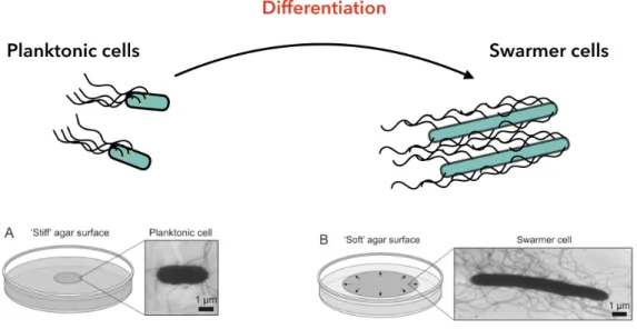
How bacteria sense surfaces to modify themselves involves one or more mechanical, physical and chemical cues [33]. During this phenotypical transition most of the Eubacteria (i.e prokaryotic cells that have specific characteristics like flagella, pilus and asexual reproduc-tion [34]) elongate, increase the number of flagella relative to planktonic cells, as depicted in Figure 1.1, and secrete a wetting agent to have a faster displacement over the surface [35]. For example, Escherichia coli elongates to twice its length, increases its mean speed (from 25 µm/s (planktonic cells) to 40 µm/s) and reduces its tumbling rate [36]. The swarmer state is the fastest known bacteria mode of surface translocation and enables the rapid colonisation of a nutrient-rich surface or a host tissue [37].
Later, the cells are irreversibly attached to the surface and the local density increases. Next, the formation of bacteria colonies takes place marking the pace of cell-to-cell communi-cation [32, 38] and the expression of the genes involved in the production of polymeric substances composing the extracellular matrix [32, 39]. At this point, the colonies should be considered as bacterial communities with complex dynamics that emerge due to their self-organisation [17].
Fig. 1.1 Differentiation from planktonic to swarmer cells. Bacteria move by a range of mechanisms. When bacteria are close to a surface they tend to switch from the swimming state (planktonic state) to a swarming state, where bacteria displace in a multicellular manner. During this differentiation cells elongate, the number of flagella on the membrane increases and bacteria tend to secrete a wetting agent. These changes are strain dependant. The electron transmission microscopy (TEM) images show the differentiation of a planktonic S. liquefacienscell (A) into its swarming phenotype (B), we can see that a over-expression of flagella and the elongation of the cells are present. In this case the phenotype change is dependent on the stiffness of the agar surface [35].
Finally, the maturation of these aggregates (colonies) into three-dimensional structures gives rise to a mature biofilm. The cycle restarts after a volume threshold is reached or at cer-tain environmental cues (e.g. depletion of oxygen or lack of nutrients), at this moment some chunks or planktonic cells from the biofilm detached [32]. The growth and decay of mature biofilms are also influenced by fluid flows on the surrounding environment [29, 40]. The established techniques to evaluate biofilm development are summarised in table 1.1. All these techniques use diverse devices that provide a surface and some sort of confinement.
Table 1.1 Biofilm formation devices
Device Technique Biofilm type Reference Microtiter plates S SAB or ALI [41–43]
Caligary device S SAB [44–46]
Ring test S SAB [47–49]
Robbins device F FFB [50, 51]
Drip-flow reactor F SAB [52, 53]
Rotary reactor F SAB [53, 54]
Flat plate reactor F SAB [55]
Flow chamber F FFB [56]
Microfluidic devices S/F SAB or FFB [26, 57]
Note: S:static. F: flow. SAB:Surface-attached FFB:Free-floating ALIB: air-liquid interface. The coupling of these devices with optical and genetic tools has enabled a tremendous progress in biofilm research [32]. Prompting the elucidation of the genetic pathways, phys-iological responses or intracellular signal transduction pathways, such as those regulated by cyclic dimeric guanosine monophosphate (d-di-GMP) that underpin biofilm develop-ment [54, 58, 59]. In the same manner, these techniques allow focusing on the understanding of interface-biofilms (solid-liquid, liquid-liquid or gas-liquid) and on their eradication [29]. Nevertheless, how bacteria attach to, transport along and interact with the interfaces is not well understood. Microfluidic systems permit the control of diverse environmental settings, allowing to study how transport, attachment, and growth of bacteria and biofilms are modified by medium geometry, fluid flows, shear rate, and surface topology. The confinement provided by these microfluidic devices has enhanced the study of the effects of steady-state flows, and more recently, the study of transient flows and how they affect bacterial behaviour near surfaces and in confinement [60–62]
Collective behaviour of bacteria in confined spaces
Recently, the confinement of bacteria and their use as model organisms in the ever-growing field of active matter has afforded the opportunity to study the dynamic assembly and col-lective motility of living self-propelled agents [63, 64]. Bacteria are low Reynolds number swimmers (Re 105) [65] with motion dominated by the viscosity of the fluid in which they swim [66]. The great majority of bacteria swim using one or more flagella, consisting of a passive helical filament connected to a rotary motor. For example, as we will discuss in Chapter 3, E.coli bears many flagella, distributed around its body, that assemble into a bundle for swimming and unbundle to re-orient in a different direction [66] as in Figure 1.2. This
type of motion is called run-and-tumble and is diffusive at large scale, just like Brownian motion [67, 68].
Fig. 1.2 Escherichia coli motion. Bacteria achieve directional movement by changing the rotation of their flagella. In a cell with peritrichous flagella, the flagella bundle when they rotate in a counter-clockwise direction, resulting in a run. However, when the flagella rotate in a clockwise direction, the flagella are no longer bundled, resulting in tumbles. The fluorescent microscopy images from swimming E.coli cells show the cells in the corresponding flagella configuration [69].
However, when bacteria are in a collective, fascinating properties are displayed, which normally originate via the interplay of individual self-propulsion and surfaces, fluid flow and surface interactions or the interaction among other individuals in the group [63, 64]. Typically, bacteria collective motion is studied under confinement with solid walls; using microfluidic chips, agar plates, Hella cells or any recipient with physical walls. More recently, these behaviours have been studied under magnetic or optical confinement using bacteria with specific phenotypes and properties.
Agar substrates
Culturing bacteria on agar plates, evaluating their growth into colonies and analysing their social behaviour is an everyday task in a microbiology lab. The use of this straightforward technique permitted the discovery of the genetic machinery of bacteria, the communication capabilities that enable the self-organisation of complex structured bacteria colonies [63] and their multicellular-organisms-like behaviours [70]. Bacteria within the colonies growing on wet agar surfaces produce a variety of collective motion patterns, see Figure 1.3.
Fig. 1.3 Collective motion on agar surfaces. A. Vortices exhibit by Paenibacillus vortex. Each plate is inoculated with bacteria that grew on different zones of the mother plate [71]. B.Instantaneous configurations at two densities of Bacillus subtilis. The velocity vectors are over-layered on the raw images of bacteria. C. Two dimensional velocity fields superimposed on color plots of n-vectors, with zero magnitude vectors are represented by a dot [72]. Thin films
One method for observing active bacterial systems is to disperse a bacterial suspension in a free-standing soap with micro-metric thickness and use micron-sized particles to track the flow [73]. Under this configuration, it has been observed that the majority of the bacterial suspension fluid self-organises into an active bacterial-film [74].
Microfluidic chips
There is a myriad of experiments that characterise the orientation of cells in a confined and dense bacterial suspension using microfluidic devices [75–79]. For example, the analysis of dense suspensions of aerobic bacteria confined in a micro-channel showed that the bacteria collective exhibits convective plumes; and on scales much larger than a cell, the presence of high-speed jets straddled by vortex streets produced by the hydrodynamic interactions between swimming cells emerges [80]. Other experiments have enabled the direct measure-ments of the flow field generated by individual swimming Escherichia coli both far from and near to a solid surface. Also, the quantification of cell-cell interactions and its link with the assemblages of bio-filaments, and flocks [81]. The emergence of self-sustained mesoscale turbulence-like motion dominated by short-range interactions [82] and the existence of a transition from quasi-two-dimensional collective swimming to three-dimensional turbulent behaviour have been described [75, 83–85]. Additionally, the presence of the alignment of neighbouring bacteria (Bacillus subtilis) in nearly close-packed populations has been observed, and named “Zooming BioNematic” (ZBN) in analogy to the molecular alignment of nematic liquid crystals [86].
Fig. 1.4 Fluid flows created by swimming bacteria in confined suspensions. A. Wioland et al. experimental work demonstrated that the flow behaviour of an active bacterial sus-pension can be controlled by tuning the length scale at which bacteria are confined [85]. B. The geometry of confinement controls the emergent collective dynamics in bacteria suspensions [76]. C. Self-organization from simulations (green) and experiments with Bacillus subtilisdense suspensions [80].
Magnetic traps
Confining magnetotactic bacteria has provided information about the rheology of the system as a function of the magnetic field applied. It has been shown that in the limit of low shear rate, the rheology exhibits a constant shear stress, called actuated stress, which depends on the swimming activity of the particles and its induced by the magnetic field and it can be positive (brake state) or negative (motor state) [87]. Some other experiments showed that these bacteria can produce magnetic crystals that align with the external magnetic field. Also, at denser suspensions the increased interaction between magnetotactic bacteria alters the ability of an individual cell to align with an applied magnetic field [88].
Fig. 1.5 Collective motion mediated by magnetic fields. A. Magnetotactic bacteria orient themselves and move along magnetic field lines. This positioning is possible because of the presence of magnetosomes, small organelles of magnetic iron material wrapped in a membrane. The alignment of the magnetosomes as a response to the magnetic field creates bacterial crystals [88]. B. Segregation of a magnetic bacteria flow in a microchannel due to the impose magnetic field.
The aforementioned techniques provide confinement and surfaces where bacteria can easily attach, and by varying the distance between walls (plates) the density of bacteria can be locally increased [89]. All of them are used to study arising collective behaviours of bacteria communities and could be used to study the transition to biofilm development on a long timescale [75, 83–85].
In this work, we addressed the feasibility of enhancing biofilm formation in a surface-less environment. Taking advantage of a relatively new confinement technique called acoustic levitation [90–92] we are able to levitate bacteria at a pressure node and confine them to form stable aggregates. The fact that acoustic levitation allows us to evaluate bacteria biofilm development without surface adherent cells as nucleation points is exciting as it changes the canonical model of biofilm development, that establishes the need of adhesion to surfaces or small cluster as nucleation points.
Acoustic trapping in levitation is defined as the immobilisation of particles and cells in the node (or antinode) of an ultrasonic standing wave field. It is a gentle way of performing contact-less manipulation [93, 94] inside cavities or other small confined spaces, creating pressure nodes that attract and hold particles and cells [95]. Commonly, acoustic frequencies in the MHz-range and structures in the range of a couple of 100 µm are used. The manipu-lation of the entities relies on their acoustic properties such as density and compressibility. This provides a robust technique that could manipulate basically any particle [94, 96]. The technique has already been used to trap latex beads [97], cancer cells [98], Janus parti-cles [96] and even suspension of beads and bacteria [99]. Also, several studies have shown that ultrasonic levitation does not have any negative effects on living cells. Hultström et al. cultured cells that had been levitated for over an hour and studied the doubling times of the cells and no direct or delayed damage could be detected on them [95, 100]. Also, Bazou et al. performed studies on mouse embryonic stem cells and confirmed that they could see no changes in gene expression after ultrasonic treatments up to one hour and the cells maintained their pluripotency [98].
It is then evident that acoustic trapping can provide confinement of suspensions in a surface-less environment that is also biocompatible. The main goal of this work is to test this technique, which could become the best, to evaluate biofilm development with no surface-adhered cells as a starting point.
In the following Chapter, we described in detail the theory behind the acoustic trapping tech-nique and the considerations that we took in the design and fabrication of the acoustic trap. We present the characterisation of the device and its ability to trap both beads and bacterial cells. Later, on Chapter 3, we present the details of the model strains of Escherichia coli we used to evaluate the clustering process that leads to a confinement of cells in levitation, followed by the disintegration processes of the floating bacteria clusters. We evaluated these processes for both motile and non-motile phenotypes of Escherichia coli, and conclude that
self-propulsion affects the disintegration of the clusters. Also, it was noted that under the confinement in levitating conditions motile bacteria exhibited a turbulent-like behaviour within the cluster, whereas non-motile bacteria did not. This behaviour is characterised by probing the mean kinetic energy and the enstrophy within a floating cluster.
Finally, with guidance from our results in Chapter 3 we present experiments on forming float-ing biofilm-like structures. To do so we used two different strains of motile Escherichia coli; one carrying a mutation on the allele ompR234 resulting in an increase in CsgA proteins levels, therefore, promoting biofilm formation and the other with a knock-out of the same allele. The results, presented in Chapter 4, show that is possible to form floating biofilm-like structures that present phenotype-dependent characteristics.
Acoustic confinement in levitation
Acoustic waves can exert forces on small particles, a fact that was discovered by August Kundt and presented as a way to measure the speed of sound in gaseous medium [101]. More than one hundred years later, in 1971, this effect was observed for biological particles in a liquid media. Dyson et al. [102] and later Baker et al. [103] reported red blood cells bands that appeared after their exposure to ultrasound. Today, this phenomenon is utilized primarily for air-levitators, where small droplets or particles can be held in air without contact [104], separation of bioparticles in a flow via acoustophoresis, as well as the capture and retention of cells or microparticles in fluids through acoustic trapping.
Acoustic trapping is based on the use of mechanical waves to manipulate particles, the parameters that allow their manipulation are density and compressibility–from the particles and the fluid. It is clear that the long wavelength, in the millimeter range, is an advantage as it allows capturing large groups of particles and also provides their capture and retention confining them away from the surface [94].
At this moment, there are several micro-systems used for acoustic trapping with a plethora of biological and non-biological applications [105, 106]. Nevertheless, the fact that these systems are complex and functional labs-on-a-chip does not imply that they are the only or most robust acoustic trapping systems. Therein, an emblematic acoustic trapping system is the multi-layered or planar resonator. The planar resonator is a vertical structure with three wavelength-matched layers (i.e. the layers should have an acoustic impedance and thickness that depends on the acoustic wavelength) [107]. The coupling layer, on the bottom of the resonator, provides efficient transmission of the waves from the piezo-ceramic transducer into the next layer of the system. The cavity or fluid layer is where the trapping of particles or cells takes place, on top of it a reflecting layer is placed to reflect the transmitted waves
and avoid their dispersion. By using operational frequencies in the order of MHz and single or multiple nodes, the fluid layer can be scaled down sufficiently to allow laminar flow conditions inside the cavity of the system, as in the design pioneered by Bazou et al. [98] One of the key goals of this thesis is to design and fabricate a trapping system based on acoustic resonances. Throughout this Chapter, an introduction to the theory behind these systems is presented, followed by the specifics of the design, fabrication and characterisation.
2.1
Acoustofluidics
Acoustofluidics is the linkage of ultrasonic waves with microfluidic systems to manipulate fluids and particles in the micro scale. In the 1930s a key study of incompressible particles in acoustic fields was published [108] and twenty years later, the forces on compressible particles in plane acoustic waves were calculated by Yosioka and Kawasima [109]. Later, these works were admirably summarized and generalized in a short paper by Gorkov [110]. At the beginning of the 1980s, a lot of work had appeared discussing the utility of acoustic waves to trap and transport passive systems. Unfortunately, as so often happens in science, the idea was left behind to experience a revival in the early 2000s, with what is known as acoustofluidics. After the new term was coined [94], seminal works from Coakley [111–114], Laurell [115, 116] and Bruus [117, 118] appeared, providing a detailed mathematical and experimental verification of how ultrasonic waves are applicable in microfluidics.
The main idea is that the wavelength (λ ) generated by the coupling of the ultrasonic frequen-cies ( f ), in the low MHz-range, and the speed of sound in water cwis typically less than 1 mm.
For that reason, it may fit submillimetric cavities and result in the formation of resonance modes. Accordingly, it has been proved that it is advantageous to operate an acoustofluidic device in its acoustic resonances [119], as they are stable, reproducible, and the spatial pat-terns are controlled by the geometry of the device. Moreover, the maximum acoustic power released by the piezo-ceramic transducer to the system arises in resonant systems, where it results in the emergence of acoustic radiation forces and acoustic streaming [115, 119].
2.1.1
Acoustic waves
Acoustic waves are mechanical and longitudinal waves, i.e. same direction of vibration as the direction of propagation, that result from an oscillation of pressure that travels through a solid,
liquid or gas in a wave pattern. They can be characterized by their wavelength λ = v/ f that depends on the media in which the wave is propagating, their frequency f , period T = 1/ f and amplitude. The acoustic wave is defined using a field that describes either the displace-ment itself ξ , the velocity of the displacedisplace-ment v, the scalar velocity potential Φ such that ~v = ~∇Φ, or the pressure changes p associated with displacing the matter. Regardless of which aspect is used to describe the acoustic wave, it will obey the wave equation, that for velocity is:
∂2v ∂2t = c
2
0∇v (2.1)
Here, c0is the speed of sound as it couples the change in position to the change in time. The
speed of sound is a material-dependent parameter and can be found from the compressibility κ and the density ρ of the media using the following relation:
c0= p1
κρ (2.2)
2.1.2
Acoustic waves interaction with suspensions
The linear wave equation for the acoustic field in a fluid can be derived using a first order perturbation theory. We recall here the derivation of Bruus [120] where the acoustic field is derived based on an equation of state describing pressure p in terms of density ρ (equa-tion 2.3), the kinematic continuity equa(equa-tion for the density (equa(equa-tion 2.4 ), and the dynamic Navier-Stokes equation for the velocity v (equation 2.5):
p= p(ρ), (2.3)
∂tρ = −∇ · (ρv), (2.4)
In the first order perturbation theory, a quiescent liquid with constant density ρ0and pressure
p0 is considered. At a given time, the fluid is disturbed by an acoustic wave-front and the
small perturbations in the density, velocity and pressure fields are described respectively by:
ρ = ρ0+ ρ1, p= p0+ c20ρ1 and v = v1. (2.6)
Later, when the equation of state is derived, it has the dimension of a squared velocity c2 0,
where c0is considered as the speed of sound in the fluid. Using the previous equations, and
neglecting the products of the first-order terms, the first-order continuity and Navier-Stokes equations are:
∂tρ1= −ρ0∇ · v1, (2.7)
ρ0∂tv1= −c20∇ρ1+ η∇2v1+ β η∇(∇ · v1) (2.8)
Following Bruus [120] we assume that there is a harmonic dependence in all fields, such that:
ρ1(r,t) = ρ1(r)e−iωt, p1(r,t) = c20ρ1(r)e−iωt and v1(r,t) = v1(r)e−iωt, (2.9)
with ω = 2π f as the angular frequency and, as stated before, f the frequency of the acoustic field. Inserting equation 2.15 into equation 2.7- 2.8 the equation of pressure is:
with k the complex wave-number given by:
k= (1 + iγ)k0= (1 + iγ)ω
c0. (2.11)
On this manner, equation 2.10 is the Helmholtz equation for a damped wave with wave-number k and angular frequency ω. Since the damping factor is γ ⌧ 1 the viscosity on the bulk part of the acoustic wave is neglected, hence, the wave equation becomes:
∇2p1= 1
c20∂
2
t p1. (2.12)
This equation shows that a pressure perturbation propagates a distance ±c0t in a time t,
therefore c0is indeed the speed of sound.
To assess the slowly evolving phenomena that arise due to acoustic waves it is necessary to use the second-order perturbation theory. According to this theory, the processes are governed by time-averaged fields, where the temporal averages of the first order fields are zero and an expansion in equations is needed:
ρ0∇ · hv2i = −∇ · hρ1v1i, (2.13)
η∇2hv2i + β η∇(∇ · hv2i) − ∇hp2i = hρ1∂tv1i + ρ0h(v1· ∇)v1i. (2.14)
The averaged second-order fields will, in general, be non-zero because of the time-averaged products of first-order terms acting as source terms on the right-side of the governing
equations. It is important to emphasize that, physically, the non-zero velocity hv2i is the
so-called acoustic streaming [121] and that from the non-zero pressure hp2i arises the acoustic
radiation force. The acoustic radiation force emerges from the scattering of acoustic waves causing acoustophoretic motion of the particles [120].
2.1.3
Resonance modes
In a geometry confined by boundary conditions, the wave equation has Eigenmodes, corre-sponding to the pattern in the acoustic field that repeats over time, and Eigenvalues, that are associated with the repetition frequency. If the system is supplied with a matched frequency to the repeating patterns in the acoustic field, more energy can be added to the system–thereby creating a resonating system.
In other words, acoustic resonances occur for certain specific frequencies ωj, j=1,2,3,(...)
An acoustic resonance at a given ωj is a state where the average acoustic energy density
(< Eac>) inside the cavity is several orders of magnitude larger than at other frequencies.
By tuning the applied frequency to one of these resonance frequencies, the acoustic forces become strong enough to enable particle manipulation. The values of the frequencies depend on the geometry of the acoustic cavity and on the material of the layers and the fluid parame-ters.
The most relevant parameters are the speed of sound in the media c0, the density of the
media ρ0and, in the same manner, of the material composing the cavity. The amplitude of
a resonance field, at a given actuation, is determined by the amount of energy that can be stored in the mode and transferred to the system. This is determined by the attenuation of the system and the coupling of the source of actuation.
In idealized systems, e.g. simulation, it is feasible to calculate possible modes for a given geometry and the use of experimental data makes predictions more accurate [122–124]. Also, there are in silico or experimental techniques to measure the acoustic field, such as the use of hydrophones [125]; but on closed systems a suitable method to measure these properties directly has not yet been invented. However, the acoustic field can be measured indirectly using the movement of particles coupling particle tracking velocimetry (PTV) in combination with mathematical models [126] as in Figure 2.1.
Fig. 2.1 Acoustic resonances in microfluidic chips. Three sets of experiments performed by Hagsater et al. [126] (A.) Experiments with 5 µm beads at 1.936 MHz acoustic resonance. The white vectors indicate the initial bead velocities pointing away from pressure anti-nodes immediately after the piezo-actuation is applied. On the bottom, the distribution of the beads on a different acoustic resonance is depicted. (B.) The acoustic and radiation forces at a 2.7 MHZ resonance show that with 5 µm particles (top) acoustic streaming can be neglected, whereas for 1 µm (bottom) it overcomes acoustic forces and the particles act as tracers of the flow. (C.) Experiments with 5 µm beads show that the geometry asymmetries on the micro-devices can change completely the energy distribution for different acoustic resonances.
2.1.4
Acoustic radiation force on small particles
A spherical micron-sized particle with radius a ⌧ λ, density ρp and compressibility κp
suspended in an inviscid fluid with density ρ0and compressibility κ0 under the influence
of an ultrasonic field of wavelength λ , will act as a weak point-scatterer of acoustic waves. The incoming wave described by a velocity potential φin will result in a scattered wave
φscpropagating away from the particle as depicted in 2.2. As a result, the total first order
acoustic field φ1is the sum of the two and it is valid for weak incoming and scattered waves.
Mathematically we have:
v1= ∇φ1= ∇φin+ ∇φsc, (2.16)
p1= iρ0ωφ1= iρ0ωφin+ iρ0ωφsc. (2.17)
Once the first-order scattered field by a given incoming field is calculated, the acoustic radiation force Fradon the particle is determined by the surface integral of the time-averaged
second-order pressure p2 and a momentum flux tensor ρhv1v1i at a fixed surface outside the
oscillating sphere, represented by the yellow arrows in Figure 2.2. The expression for the radiation force becomes [120]:
Frad= − Z δ Ωda{hp2in + ρ0h(n · v1)v1i} (2.18) = − Z δ Ωda ⇢ 1 2κ0hp 2 1i − 1 2ρ0hv 2 1i $ n+ ρ0h(n · v1) v1i % , (2.19)
where n is a unit vector pointing outwards perpendicular to the element of an area da. In this problem there are no body forces, thus, any fixed surface ∂ Ω encompassing the spherical particle experiences the same force. To derive the rest of the equations, scattering theory is used; for a detailed description of this, see [127]. The scattered field φscfrom a point
scatterer (particle) at the centre of the system is represented by a time-retarded multi-pole expansion. In the far field region, the monopole (φmp) and dipole (φd p) components dominate
and according to the first-order scattering theory φscthe field must be proportional to the
Fig. 2.2 Acoustic radiation force. On the left, a sketch of the far-field region r ⌧ λ of an incoming acoustic wave φin (vertical purple line) of wavelength λ scattering off a small
particle (pink dot) with radius a ⌧ λ, prompting the outgoing scattered wave φsc(purple
circles and arrows). The resulting first-order wave is φ1= φin+ φsc. On the right it is shown
a compressible spherical particle (pink) of radius a, compressibility κp, and density ρp,
surrounded by the compressible inviscid bulk fluid of compressibility κ0and density ρ0. The
fluid is divided into the near-field region for r ⌧ λ, with the instantaneous field φsc(t), and
the far-field region with the time-retarded field φsc(t −cr0). The radiation force, Frad(blue
arrows), evaluated at any surface in the far-field region (dashed circle), equals that evaluated at the surface of the sphere (yellow arrows) [120].
The implementation of the scattering theory allows the radiation force to be expressed in terms of the incoming acoustic wave evaluated at the particle position and can be used to derive two complex scattering coefficients f1and f2 that represent, respectively, a monopolar
scattering due to the presence of a compressible particle, and a dipolar scattering related to the translation of the particle. Thus f2depends on the viscosity of the fluid. Thanks to
this implementation, the equation for the radiation force acting on a small particle (a & λ) is:
Frad= −4π 3 a 3∇1 2Re[ f1]κ0⌦ p 2 in↵ − 3 4Re[ f2]ρ0⌦v 2 in ↵ $ , (2.20) with: f1( ˜κ) = 1 −κp κ0 (2.21) f2( ˜ρ) = 2(ρ − 1) ρ + 1 . (2.22)
In summary, the resulting radiation force Fradon a small, spherical particle in an inviscid
fluid is the gradient of an acoustic potential:
Frad= −∇Urad. (2.23)
In the case of a 1D planar standing λ /2-wave with, p1(z) = pacos(kz) where: k = 2π/λ =ω/c0
and w = λ /2 being w the channel width, the radiation force from such field is given by:
Fzrad= 4πΦ(κ, ρ)ka3Eacsin(2kz), (2.24)
where Eacthe acoustic energy density is:
Eac=
Pa2 4ρ0c20,
(2.25)
and the so-called acoustophoretic contrast factor:
Φ( ˜κ, ˜ρ) =1 3 5 ˜ρ − 2 2 ˜ρ + 1 − ˜κ $ . (2.26)
2.1.5
Energy density in a piezo-transducer
In applications of the acoustic radiation force in trapping systems is important to remember the linear relation that exists between the applied peak-to-peak voltage Upp, that produces
density that is generated.
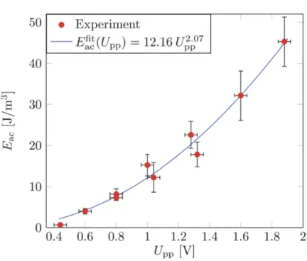
By tracking the y-position over time of polystyrene micro-beads Barnkob et al. [117] showed that at a fixed driving frequency ( f = 1.99MHz) the acoustic energy density (Eac) as a
func-tion of the peak-to-peak value Upp(0.5-1.9 V) scales as a power law of the form Eac∝ (Upp2.07)
as depicted in Figure 2.3. This is close to the power law of two, which is expected since the acoustic pressure delivered by the piezo-transducer is proportional to the applied voltage and, the acoustic energy density proportional to the square of the pressure [119, 128]:
Eac∝ p2a∝ Upp2 (2.27)
Fig. 2.3 Measured acoustic energy density Eacversus applied peak-to-peak voltage Uppon
the piezo -transducer (points) for α = 1. A power law fit (full line) to the data is close to the expected square law, Eac∝ Upp2 . From this figure, Barnkob et al. [117] were able to extract
2.1.6
Secondary radiation force
The secondary radiation force–also known as Bjerkness force when acting on gas bubbles or Köning forces when acting on solid particles–is an inter-particle force [129]. It can be attractive or repulsive and depends on the distance between particles. In addition, its amplitude is two orders of magnitude smaller than the primary radiation force (Frad). We
already discussed that a particle acts as a scattering point, hence, the acoustic waves coming from the emitter will scatter in all the particles on the suspension. The secondary force in the case of a plane wave incident field in a suspension is given by [130]:
Fsec= 4πa6 (ρp− ρ)2(3 cos2θ − 1) 6ρd4 v2(x) − ω2ρ(κp− κ)2 9d2 p2(x) $ . (2.28)
Here ω is the angular frequency, d is the distance between particles (centre-centre) and θ is the angle between the axis of the incident wave and the centre-line connecting the two particles.
This definition of the force is such that a negative sign should be interpreted as an attractive force between the particles [131]. The secondary radiation force scales heavily with the distance between the particles as the magnitude drops off so rapidly with particle spacing, the effects of the secondary radiation force can be ignored in many cases. Nevertheless, when particles are trapped in a tight cluster the force has a significant contribution [132].
Interestingly, the secondary radiation force has two terms; one that is always attractive, and one that is angle-dependent. As the angle-dependent term decreases faster with the distance between particles there will be an equilibrium-distance to which a particle is drawn. The equilibrium distance will be angle dependent, such that at some angles the particles will tend to be as close as possible, whereas at other angles a small separation will be preferential. While the formula for the force is given for two identical particles, in reality, there will be, of course, secondary forces between particles with different sizes and properties [133].
2.1.7
Acoustic streaming
The acoustic field imposed on a suspension will not only create forces on the particles but it will also create forces on the media itself. This phenomenon is called acoustic streaming, and it is defined as the generation of fluid flows by sound. Here, the sound plays the leading role and the flow is a by-product [121]. Furthermore, acoustic flow generation shows features symmetrical with those of aerodynamic sound generation, i.e. not only can a jet generate sound, but also sound can generate a jet.
The first theoretical model to thoroughly describe acoustic streaming flows was derived by Rayleigh in 1884 [134]. In his work, Rayleigh treats the cases of streaming that were observed experimentally by Faraday [135] and Dvorak [136]. Two cases of streaming that were observed by Faraday are related to the observations on the patterns assumed by sand and fine powders on Chladni’s vibrating plates [137]. Also, Rayleigh analysed Dvorak’s observations which consisted on the circulation of air currents in a Kundt’s tube [134, 135]. Streaming flows vary greatly depending on the mechanism behind the attenuation of the acoustic wave. The variations include the velocity of the flow, the length scale of the flow and the geometry of the same. The velocity variation could be from being on the order of mm, as in the case of slow streaming, up to velocities on the order of cm or more for fast streaming. For example, in the case of microstreaming the length scale variations are in the order of mm, whereas in bulk streaming up to the order of cm where the flow geometry may take the form of a jet or of vortices [138].
Another example is the boundary-layer driven acoustic streaming. This type of streaming is formed by the viscous dissipation of the acoustic energy into the boundary layer of a fluid along any solid boundary that has a length greater (in the direction of acoustic propagation) than a quarter of the acoustic wavelength [139]. In addition, the streaming flow is typically observed in fluid cavities where at least one dimension, perpendicular to the direction of acoustic propagation, is comparable in size to the acoustic wavelength.
The main types of streaming flows that have been described in the literature can be classified as:
i. Schlichting streaming.Described as the viscous dissipation that results in a steady mo-mentum flux that arises in a system that has a standing wave parallel to the surface. It is typically oriented from the pressure anti-nodes to the pressure nodes close to the solid
boundary, see Figure 2.4A [140].
ii. Rayleigh streaming This type of streaming, depicted in Figure 2.4A, appears once Schlichting streaming is established. The powerful inner boundary layer streaming flow generates counter rotating streaming vortices within the bulk of the fluid [134].
iii. Eckart streaming.Formerly called "quartz wind" is the flow formed by the dissipation of acoustic energy into the bulk of a fluid, as seen in Figure 2.4B. As an acoustic wave propagates through a fluid, a part of the acoustic energy is absorbed by the fluid at a rate proportional to the square of its frequency. The amplitude of the acoustic wave becomes attenuated causing the acoustic pressure amplitude to decrease with distance from the acous-tic source [138]. The loss of acousacous-tic energy results in a steady momentum flux, forming a jet of fluid inside the acoustic beam in the direction of the acoustic propagation. When a fluid jet is formed within the confinement of a micro chamber vorticity ensue, resulting in a fluid circulation either within the entire chamber or just on a specific region [138]. Matsuda, Kamakura and Maezawa showed that the Eckart streaming will only take place in microfluidic devices when high-frequency ultrasound is propagated along a dimension on the order of a millimetre long [141].
iv. Cavitation microstreaming.This particular form of boundary-layer-induced streaming arises by the viscous dissipation of acoustic energy in the boundary layer of a stable oscil-lating microbubble [142]. The forced oscillation of microbubbles, sonicated at or near their resonance frequencies, results in the local amplification of the first order velocity [139]. It is an altogether different concept from that of a fluid jet formed by the destructive cavitation of a bubble, which despite being an acoustically induced flow is not a form of acoustic streaming, see Figure 2.4C [138, 139].
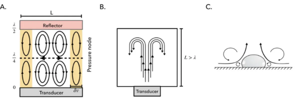
Fig. 2.4 Types of streaming described in literature A. A λ
2 resonator with inner
Schlicht-ing boundary layer streamSchlicht-ing within the viscous boundary layer (yellow regions) with thickness δ v and outer (Rayleigh) boundary layer streaming within the bulk of the fluid (white region). In the plane of the pressure node, the outer boundary layer streaming is directed outwards counteracting the lateral component of Frad. B. Eckart streaming in a
resonator much larger than the wavelength (L > λ ). The forward streaming jet induces backflow typical for Eckart streaming. [143] C. Cavitation microstreaming due to spherical volume oscillations of a gas bubble resting on a solid boundary. Here the cross-section through the centre of the bubble is shown. Due to the hemi-spherical shape of the bubble only half of the typical streaming pattern is formed [144].
As we can see, acoustic streaming is a well-known phenomenon that depends on the geometry of the cavity where arises (see Figure 2.5). Nevertheless, due to its many forms, it is often considered a nuisance since it is present inside many acoustically driven microfluidic devices where it could be counter-productive. While in some cases it is indeed a problematic phe-nomenon [145–147], when used correctly it can be very useful and could help overcoming some of the challenges presented by low Reynolds number flows in microfluidics [138, 143]. Rayleigh streaming plays an important role on half-wavelength chambers setting a lower limit on the particle size that can be manipulated by the primary radiation force in a standing wave [138]. This is particularly relevant when the streaming direction is opposite to the direction of the radiation force. For example, Spengler et al. [148] observed that whilst larger (10 µm) particles became agglomerated in the centre of the pressure nodal plane, smaller particles of the order of one micrometre did not, as the drag from the streaming flow overcame the lateral radiation force. Later, it was shown that beads of intermediate size are able to overcome the drag from Rayleigh streaming only after they have formed mini-aggregates off-axis at the edges of the acoustic fields, implying that the depletion of beads in that plane is caused by the increase of the effective volume of the mini-aggregates relative to single beads [99]. Therefore, the increase in volume has a stronger effect on the volume-dependent
radiation force than on the radius-dependent viscous drag from acoustic streaming [148–150]. In addition, Martin and Minor found that an increase either on the frequency or pressure amplitude resulted in an increase of the streaming velocity, whereas halving the chamber thickness (to obtain a14λ resonance) had as a consequence a reduced streaming velocity [151]. Posterior to this, a more detailed analysis of the size-dependent cross-over from radiation force dominance to streaming dominance was carried out by Barnkob et al. [117] see Fig-ure 2.5.
They concluded that the theoretical threshold, based on experimental data, defined as the particle size for which the two forces were equal in magnitude, corresponds to a particle with diameter of 2.6 µm at a driving frequency of 2 MHz. Also they found that the threshold particle size is proportional to p1f, where f is the driving frequency [152].
As discussed before Eckart streaming is not the dominant form of acoustic streaming observed in microfluidic devices, however, if the dimensions of the channel, or chamber, parallel to the propagation direction of the acoustic wave are of scale > 1 mm it may occur. When it comes to cavitation micro-streaming, typical applications are the generation of whole scale flows and the generation of highly targeted flows used in micromixing and cell membrane sonoporation.
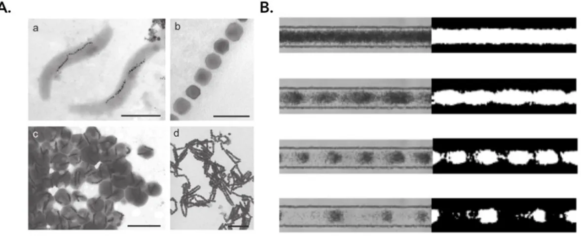
Fig. 2.5 Acoustic streaming patterns in different geometries of the acoustic resonant cavity, visualized by making an overlay of a series of frames from a video clip. The width is between 300 and 350 µm in all cavities, and the driving frequency is between 2.1 and 2.6 MHz. The streaming is tracked by 1 µm fluorescent beads and the trapped cluster in the centre of each cavity contains 5 µm beads in (A) and (B), and 10 µm cells in (C). There are only 1 mm beads present in (D). These experiments correspond to Rayleigh streaming [138, 153]
2.2
Acoustic confinement
To confine living or non-living matter in microgravity like conditions, acoustic trapping systems work under the basis of the acoustic radiation forces that arise when a standing wave is set up in a microchannel or in the cavity where a suspension is placed. To create a standing wave inside a cavity or micro-channel, the driving frequency must meet a resonance criterion as follows:
w= nc0 2 f = n
λ
2. (2.29)
Where w is the width of the channel or cavity, n is the number of pressure nodes in the standing wave, c0 is the speed of sound in the fluid, f is the acoustic frequency and λ
the wavelength of the acoustic input. The acoustic radiation forces will promote the dis-placement of objects either to the point of maximum or minimal acoustic potential in the standing wave (Figure 2.6), depending on the acoustic properties of the species being handled. On a 1D planar standing wave, the acoustic radiation force, as expressed in Equation 2.22, shows that the radiation force can be expressed as the gradient of the acoustic potential Urad
where the acoustic potential is given by:
Urad= 4π 3 a 3f 11 2κ0hP 2 ini − f2 3 4ρ0hv 2 ini $ , (2.30) where hP2
ini and hv2ini are the time averages of the incoming pressure and velocity fields
squared, and the scattering coefficient f1 and f2 relate compressibility and density, of the
particles and the medium, respectively. These characteristics determine the position of the entities to be handled in the potential. Most cells and micro particles with density and compressibility lower than the surrounding medium will move to the point of minimal acoustic potential, implying that they will displace towards the pressure node of the standing wave.
Fig. 2.6 Left: Distribution of the force(solid-line) and pressure (dotted-line) in a standing wave when the distance between the emitter and the reflector is such that a node can be created n=1. Right: the corresponding acoustic potential.
An effective trapping requires a local acoustic potential with high gradient so it can provide trapping even against a background flow. The secondary forces (short distance forces) attract the particles to each other and enhance the formation of stable particle clusters [130].
2.3
Design and fabrication of the acoustic resonator
An important part of this work has been device design. It is a key engineering challenge, due to the fact that in order to make efficient acoustic devices (for ultrasonic cell manipulation), there are several considerations that need to be taken into account. When designing an ultrasonic manipulation device, especially for half-wavelength layered resonators, like the one used throughout this thesis or the ones used by Ohlin et al. [143] or Bazou et al. [98], the first consideration to bear in mind is the size range of the cells to be manipulated. Smaller particles (or cells) require higher operating frequencies to attain the same acoustic radiation forces than the one required by larger particles.
The principal aim of this work is to confine bacteria cells in a levitating environment. There-fore we took into account the dimension of bacteria which are: 3 µm long and 1 µm width. Generally 1-10 MHz ultrasound is suitable for manipulation of 1-20 µm entities, that is the reason why the resonators were designed to work in a 2-5 MHz frequency interval. This implies that the nominal frequency of the transducer needs to be between this range.
Also, it is important to heed whether to work in a single-pressure-node or a multi-node configuration. The desired configuration, no matter which, is given by the distance (w) between the emitter (matching layer) and the reflector (top layer), and it is also related to the frequency at which the resonator is driven, as the wavelength of the emitted wave is given by:
λ =c0
f , (2.31)
and the distance between emitter and reflector layers relates the number of nodes n with the wavelength as in Equation 2.29
Typically the layered resonator is structured by different layers as seen in Figure 2.7. First, the piezo ceramic transducer that generates the sound is attached to the coupling layer, which is needed to get good acoustic transmission into the system and acts as the bottom of the resonator chamber. Next, the fluid layer containing the cells or beads suspension. This layer either can have inlets and outlets or be completely sealed. At the other end of the system the reflector layer it is placed. This last layer is responsible for reflecting the incoming wave back into the fluid layer. The interference of the incoming and the reflecting wave gives rise to a standing wave [115]. Sometimes a second transducer can be used as the reflection layer [154]. It has been shown in simulations that a good resonator should have a matching layer of a quarter wavelength, a fluid layer of half a wavelength and a reflector layer of a quarter wavelength thickness. This configuration results in a pressure minimum in the centre of the cavity and a pressure maximum at the channel wall [155].
Fig. 2.7 Components of the acoustic resonator. Classic configurations of a layered res-onator with either a single transducer and a reflector layer or two opposing transducers [115]. To summarize, for our designs we kept in mind the aforementioned characteristics. We selected the single pressure node configuration because this makes imaging less complicated and prevents the interaction between bacteria clusters at different nodal planes. Additionally, since the choice of material plays an important role as well, we used a well-balanced combi-nation of materials to achieve a quality system as described by Lenshof et al. [115]
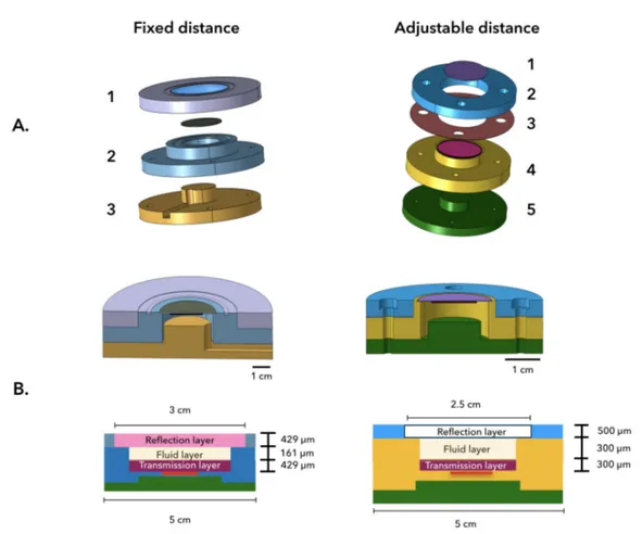
We designed two different resonators, the first one has a fixed distance and frequency; within its cavity a standing wave with a single-pressure node is created. The second one has a removable spacer, by changing the thickness of the spacer the distance between parallel plates can be modified. The thickness of the spacer determines the number of pressure nodes that arise within the cavity of the resonator. The detailed configurations of our layered resonators are presented next (see Figure 2.8):
Fixed distance
The resonator is composed by three main layers: the reflection layer is a 3D-printed lid that wraps half of the resonator and holds in place a circular Quartz-slide 250 µm thick. The emis-sion layer, includes a circular Wrap-around Feedback Piezo-ceramic transducer (Pz-26) from Meggit, with a nominal frequency of 4.6 MHz, that is glued with a water soluble conductive adhesive gel (Tensive) to a 3 cm2 circular silicon (Si) wafer with 250 µm thickness. The
wafer is fixed, with Epoxy, to a hollow cylindrical shape made of stainless-steel. The cylinder has 161 µm height (h) and a 1.3 cm radius (r). The Si wafer creates the bottom of the cavity, where the fluid layer is deposited, and the wall is the stainless-steel cylinder. At the bottom, a hat-like stainless-steel structure with a slot acts as a support for the complete resonator. This bottom layer keeps the system level and eases the manipulation on the microscope; the slot provides a place for the wires and cables that connect the transducer.
Adjustable distance
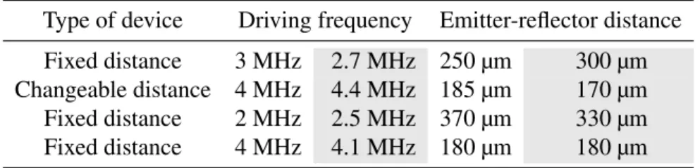
The resonator has five components: the emission plate, where another Wrap-around trans-ducer (Pz-26) this time with a nominal resonance of 3 MHz is glued, as described before, to a circular Si wafer with a 5 cm2area and 200 µm thickness. This wafer is firmly fixed into the hollow cilynder structure whose base is a stainless-steel disk. On top of it a Mylar spacer is placed. The thickness of the spacer has to be half the wavelength of sound in water at the resonant frequency, which in our case was 250 µm thick. Over the Mylar spacer, a stainless steel ring is placed, the ring creates a cavity between the emission and the reflection layer that comes on top. The reflection layer is a 500 µm thick Quartz-slide permanently attached to an acrylic lid. As on the previous design, at the bottom a hat-like structure is placed. It is important to remember that the resonators where fabricated from scratch. The stainless-steel structures were performed at the machine-shop from the laboratory and the assembly of the pieces was done by hand. For these reasons, the dimension that were planned for each design sometimes were not completely accurate. In table 2.1 the theoretical dimensions versus the experimentally obtained (gray columns) ones are summarised:
Table 2.1 Dimensions of the resonators.
Type of device Driving frequency Emitter-reflector distance Fixed distance 3 MHz 2.7 MHz 250 µm 300 µm Changeable distance 4 MHz 4.4 MHz 185 µm 170 µm Fixed distance 2 MHz 2.5 MHz 370 µm 330 µm Fixed distance 4 MHz 4.1 MHz 180 µm 180 µm
Fig. 2.8 Components of the acoustic resonator. A. 3D drawings of the two types of lay-ered resonators designed for this work: a fixed distance one and another with modifiable transmission-reflector layer distance (w). The fixed distance configuration comprises three main layers. 1. The reflector layer, that corresponds to a 3-D printed lid that has a permanently fixed Quartz-slide. The Quartz-slide permits optical access for microscopic visualization. 2. Next, the transmission layer that comprises the Si wafer holding the transducer, the wafer is fixed to a hollow cylinder with h=161 µm and r=1.3 cm. 3. At the bottom a hat-like stainless steel supporting structure that holds the system and makes the manipulation on the microscope easier. On the right, the second configuration shows the adjustable distance resonator. The resonator is formed by five layers: 1. The reflection layer is a quartz-slide permanently attached to an acrylic lid. 2. A stainless steel ring is placed on top of the Mylar spacer (3.) that is placed on top of the steel framework holding the emission plate. 4. The emission plate comprises a transducer with a 3MHz nominal resonance glued to a circular Si wafer with a 5 cm2area and 200 µm thickness. The wafer is firmly fixed into a stainless-steel structure. 5. Finally, at the bottom, the same hat-like structure as on the other design. Note that in both resonators there is a cavity (or pool) where the suspension is poured. B.Schematic diagram showing the real thickness of the three main layers for the resonators that we made. Not always they match the theoretical ones, nevertheless, because stainless steel and quartz have high-quality values the systems works and can trap beads in levitation.
2.4
Characterization of the acoustic trap
The first part of this section was performed in concert with Ludovic Bellebon as part of his master thesis [156] developed during the summer of 2017. The main goal was to measure the acoustic energy density of our acoustic resonator. The approach that was used is based on the z-position temporal tracking of latex and silica micro-beads in the cavity of the resonator. To get to know the acoustic energy density (equation 2.25) it is necessary to know the velocity of the particle during its z-displacement from the bottom of the resonator’s cavity towards the pressure node of the standing wave. For that reason, a well known optical phenomenon known as Airy patterns was used. Airy disks are a bright region in the centre of the diffraction pattern resulting from a uniformly-illuminated circular aperture, which together with the series of concentric bright rings around it, is called Airy pattern [157].
When we observe an object in the microscope and it is completely sharp it implies that it is localized on the observation plane. Whereas, when it is not, the object appears out of focus, blurry and some out-of-focus-halos surrounding it appear (Airy patterns). From these observations, we can get that the further an object is from the observation plane the blurriest it gets and the diameter of the surrounding halos increases.
This optical aberration phenomenon was used to characterized the acoustic trap that has a transducer working at a nominal frequency of 3 MHz (λ =500 µm). Since, as stated be-fore, the resonator has a configuration that gives a single-pressure node standing wave. In theory, the distance that should exist between the plates of the resonator is w=(λ /2)=250 µm. Nevertheless, due to fabrication constraints the distance between plates is 300 µm. The best driving frequency, found experimentally, is 2.7 MHz, that matches with a 277 µme inter-plates distance. Even with these slight changes in the configuration, we can be sure that the pressure node is near the cavity centre as we measure the focal plane experimentally using optical microscopy.
Remembering equations 2.24- 2.26 we can see that the acoustic contrast factor Φ character-izes the compressibility and density of the particles. Their values determine the position of the particles in the potential well (Figure 2.6); if, for example, Φ > 0 particles will migrate toward the nodes whereas if it is Φ < 0 they will migrate to the anti-nodes. The properties playing a central role in the characterization of the resonator are the density ρ of the particles and the fluid, and their compressibility κ.
Considering that a particle in a suspension subjected to an acoustic field is affected by the buoyancy force, the Stokes force FS and the acoustic radiation force Frad. Following the
description made by Dron et al. [158] the buoyancy force can be neglected, therefore:
Frad= FS. (2.32)
π AEack
3
pΦsin(2kz)ez= 3πdpUFez. (2.33)
Re-arranging the terms the focusing speed of a particle within the cavity is:
uF(z) =
Eacd2pΦk
12µ sin(2kz). (2.34)
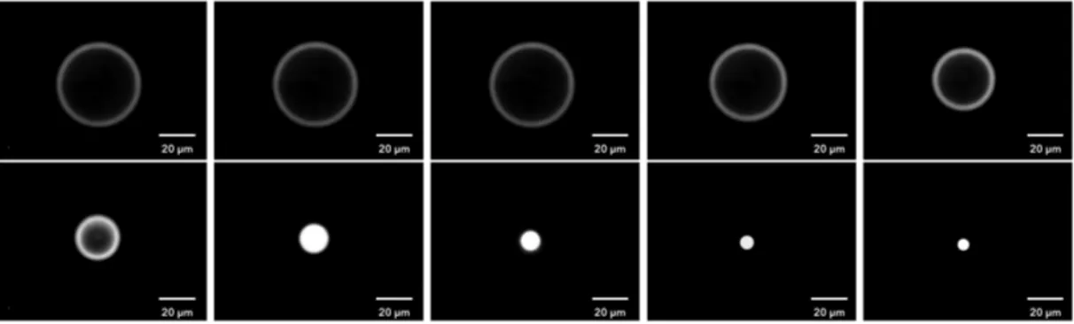
The focusing speed was determined experimentally by following the changes in the diameter of the Airy disks for several particles. The diameter of the ring was followed from the bottom of the cavity (out of focus ring) towards the nodal plane (sharp particle) as in Figure 2.9.
Fig. 2.9 Airy disk evolution during the migration of a latex bead towards the levitation-plane (nodal plane). Just one latex bead was selected for the z-migration, each image was taken 1 second apart, the Voltage applied during this experiment was 10 Upp.