SIMULATION STRATEGIES FOR OPTIMAL DETECTION OF REGIONAL CLIMATE MODEL RESPONSE
TO PARAMETER MODIFICATIONS
DISSERTATION
PRESENTED
AS PARTIAL REQUIREMENT OF THE DOCTORATE OF EARTH AND ATMOSPHERIC SCIENCES
BY
LEO SEPAROVIC
UNIVERSITÉ DU QUÉBEC À MONTRÉAL Service des bibliothèques .
Avertissement
La diffusion de cette thèse se fait dans le respect des droits de son auteur, qui a signé le formulaire Autorisation de reproduire et de diffuser un travail de recherche de cycles supérieurs (SDU-522- Rév.01-2006). Cette autorisation stipule que «conformément à l'article 11 du Règlement no 8 des études de cycles supérieurs, [l'auteur] concède
à
l'Université du Québecà
Montréal une licence non · exclusive d'utilisation et de publication de la totalité ou d'une partie importante de [son] travail de recherche pour des fins pédagogiques et non commerciales. Plus précisément, [l'auteur] autorise l'Université du Québec à Montréalà reproduire, diffuser, prêter, distribuer ou vendre des
copies de [son] travail de rechercheà
des fins non commerciales sur quelque support que ce soit, y compris l'Internet. Cette licence et cette autorisation n'entraînent pas une renonciation de [la] part [de l'auteur]à
[ses] droits moraux nià
[ses] droits de propriété intellectuelle. Sauf entente contraire, [l'auteur] conserve la liberté de diffuser et de commercialiser ou non ce travail dont [il] possède un exemplaire.» ·APPROCHES STRATÉGIQUES POUR DÉTECTER DE FAÇON OPTIMALE
LA RÉPONSE SIMULÉE PAR UN MODÈLE RÉGIONAL DU CLIMAT
SOUMIS
À DES
MODIFICATIONS DE SES PARAMÈTRESTHÈSE PRÉSENTÉE
COMME EXIGENCE PARTIELLE
DU DOCTORAT EN SCIENCES DE LA TERRE ET DE L'ATMOSPHÈRE
PAR LEO SEPAROVIC
REMERCIEMENTS
Je tien tout d'abord à remercier mon directeur de thèse, Dr. Ramon de Ella,
pour sa patience et ses conseils précieux. Ce travail fut d'autant plus agréable grâce à
ses nombreux encouragements et le soutient qu'il m'a apporté tout au long du projet.
Mes remerciements vont également à mon co-directeur de thèse, Prof. René
Laprise, qui a partagé avec moi ses brillantes intuitions. J'ai aussi grandement apprécié
sa gentillesse et sa constante disponibilité.
Je remercie aussi Mme Katja Winger pour son aide technique lors de la production
de simulations avec le Modèle Régional Canadien du Climat.
Pour ses encouragements et son assistance morale qui m'ont permis de rédiger
CONTENTS
LIST OF FIGURES IX
LIST OF TABLES . xiii
LIST OF ACRONYNIS xv
RÉSUMÉ . . xvii
ABSTRACT xix
INTRODUCTIO 1
CHAPTER I
IMPACT OF SPECTRAL NUDGING AND DOMAIN SIZE IN STUDIES OF
RCM RESPONSE TO PARAMETER MODIFICATION 11
1.1 Introduction. . . . . 14
1.2 Experimental design 17
1.2.1 Model description
1.2.2 Experiments
1.3 Results . . . . . . .
1.3.1 Spread of differences excited by perturbations . 1.3.2 Noise level in the differences
1.3.3 Signal PlO in winter .
1.3.4 Signal PlO in summ r 1.3.5 Signal POl in summer
1.3.6 Rule of thumb for the minimum ensemble size 1.4 Summary and conclusions . . . . . . . . . . . .
17 17 19 19 21 23 26 27 29 32
1.5 Appendix: Optimization of sample sizes for the test of the difference of mearis 34 1.6 Appendix: Test for the differences of signals . . . . . . . . . . . . . 35 CHAPTER II
A THEORETICAL FRAMEWORK FOR ANALYSIS OF TEMPORAL VARI-ABILITY OF RCM RESPONSE TO PARAMETER MODIFICATION . . . 51
2.1 Introduction . . . . . . . . . . . . . . . · . . . . . . . . . .. . . . 54 56 2.2 Reproducible and irreproducible components of an RCM simulation
2.2.1 General assumptions . . . . . . . . . . . . . . . . . . . . . . . 56 2.2.2 Definition of the reproducible and irreproducible components 57 2.2.3 Decomposition of variance . . . . . . . . . . . . . 59 2.2.4 Redistribution between reproducible and irreproducible variances . 61 2.2.5 Estimation of the climatological mean from ensemble integrations 63 2.3 Analysis of the RCM response to modification. . . . . . . . . . . . . . 68
2.3.1 Reproducible and irreproducible components of the RCM response to modification . . . . . . . . . . . . 68
2.3.2 Analysis of the variance of response 69
2.3.3 Estimation of the reproducible and irreproducible time variance com-ponents from two ensemble members . . . . 72 2.3.4 Estimation of the difference of RCM means 74
2.4 Sorne examples . . . . . 79
2.4.1 Model and experiments 79
2.4.2 CRCM5 reproducible and irreproducible components . 81 2.4.3 Response of the CRCM5 time-av rage to deep-convection parameter
perturbation . . . . . . . . . . . . . . . . . . . . . . . 84 2.4.4 CRCM5 transient response to deep-convection parameter perturbation 85 2.5 Summary and discussion . .. .. .. .. . . . .
2.6 Appendix: Variance of the time-ensemble rn an CONCLUSION . REFERENCES . 89 92 105 112
LIST OF
FIGURES
Figure
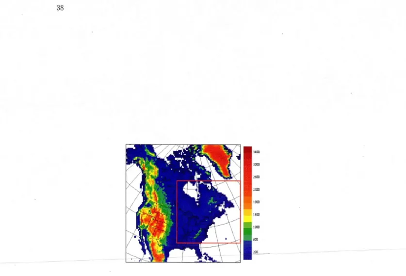
1.1 Topography of the two CRCM5 computational domains, including the lateral boundary relaxation zone. The large domain is used in the SYNA
Page
and SYSN experiments and the smaller domain in the SYDS experiment. 38 1.2 TheRMS difference between CRCM5 individual simulations for
seasonal-average (a) precipitation and (b) 2 rn-temperature as a function of the experimental setup and season. The black marks display the rmsd in seasonal averages among the ensemble members of the mode! MOO (Table 1.1); they are triggerecl by interna! variability and are obtainecl as follows: from 10 ensemble members 5 pairs of seasonal averages are selected, for each pair the rmsd is plotted. The coloured marks show the realizations of the rmsd between ensemble members of MOO and MOl (MIO); they are triggered by parameter perturbations (red) POl and (blue) PlO. . . . . . 39 1.3 Sample standard deviation (Eq. 1.1) of the sensitivity of the CRCM5
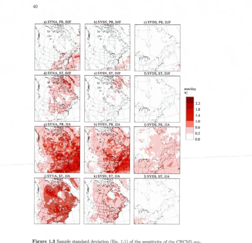
sea-sonal average to parameter perturbation PlO (Table 1.1). The sensitivi-ties are measured as the differences between members of the perturbed-parameter mode! MlO and members of the control mode! MOO ensem-bles, as a function of experimental setup, variable and season: (a, d, g, j) SYNA, (b, e, h, k) SYSN, (c, f, i, l) SYDS, (a, b, c, g, h, i) seasonal precipitation, (d, e, f, j, k, 1) 2 rn-temperature, (a-f) DJF, (g-1) JJA. . . 40 1.4 Difference of the ensemble mean winter-average (DJF) precipitation
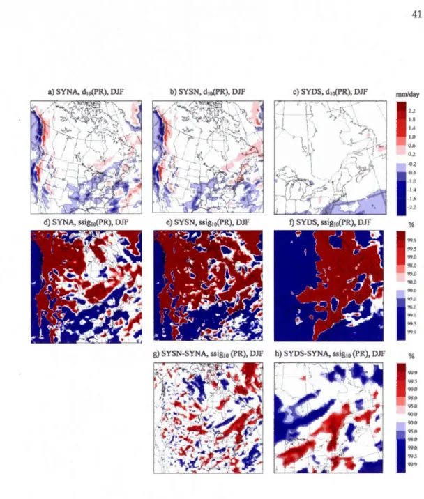
(sig-nal) due to the perturbation PlO (Table 1.1) in (a) SYNA, (b) SYSN and ( c) SYDS experiments and statistical significance of the responses (cl, e, and f, respective! y); statistical significance of the difference of the signais (g) between SYSN and SYN A and h between SYDS and SYN A experiments. . . . . . . . . . . . . . . . 41 1.5 Same as in Fig. 4 but for winter 2 rn-temperature (DJF). 42 1.6 Same as in Fig. 4 but for summer 2 rn-temperature (JJA). . 43 1.7 Same as in Fig. 4 but for the signais induced by the perturbation POl
1.8 Same as in Fig. 4 but for the signals induced by the perturbation POl for summer 2 rn-temperature (JJA). . . . . . . . . . . . . . . . . . . 45
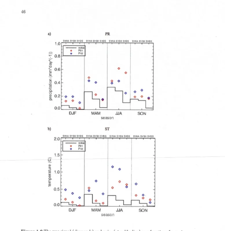
1.9 The rms signal ( diamonds) and noise ( step-like line) as a function of ex-perimental setup and season for seasonal-average (a) precipitation and (b) 2 rn-temperature. Signal is estirnated as the rms difference of ensem-ble means of the perturbed-parameter (red) MOl and (blue) MlO model and control rnodel MOO (Table 1.1). Noise is measured with the standard deviation of the difference of ensemble means. . . . . . . . . . . . . 46
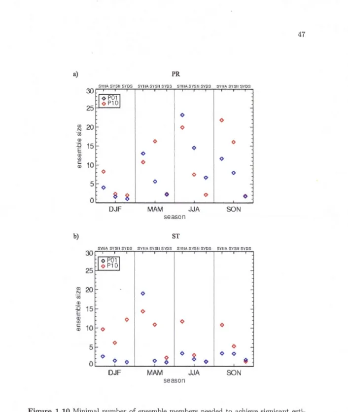
1.10 Minimalnumber of ensemble members needed to achieve signicant esti-mates at 95% level for the signals induced by the perturbations (r-ed) POl and (blue) PlO, as a function of season and experimental setup, as derived hom the rule of thumb in Eq. (1.5); seasonal-average (a) precipitation and (b) 2 Ill-temperature. . . . . . . . . . . . . . . . . . . . . . . . . . 47
1.11 Statistical signicance derived from the two-sided test of the difference of means of two samples of unequal sample sizes; the size of the first sample is kept constant and the size of the second is increased by the factor b (abscissa), as in Eq. (1.7). Plots are drawn for selected signal-to-noise ratios (Eq. 1.9). . . . . . . . . . . . . . . . . . . . . . . . . . . . 48
2.1 Illustration of the time series obtained from an ensemble of elima te model simulations. Colurnns stand for tirne series obtained from individual rnembers and may represent daily or seasonal averages. Rows represent the realizations obtained h·om ensemble members at a given time. The only difference between members is in the initial conditions. The lines on the top and right illustrate the typical behaviour of the time mean and ensemble mean, respectively. The black lines are for the case of RCMs and GCMs and red lines represent CGCMs. Note that for the case of ensemble mean the annual cycle is neglected. . . . . . . . . . . . . . . . 95
2.2 Decomposition of the time standard deviation of the control CRCM5 JJA 2 m-temperatures into the reproducible and irreproducible components (Eq. 2.11): time standard deviation at, the reproducible component a! and the irreproducible component a 6 ; (a, b, c) MYN A and ( d, e, f) MYSN experiment. . . . . . . . . . . . . . . . . . . . . . . . . . . . 96
2.3 Ratio of time standard deviations at of JJA 2 rn-temperatures between the control MYSN and control NIYNA simulations. . . . . . . . . . 97
2.4 Reproducibility ratio of the JJA 2 m-temperatures (Eq. 2.14) in the control CRCM5: (a) MYNA, (b) MYSN.. . . . . . . . . . . . . . 98
2.5 Difference of 1993-2002 JJA-average CRCM5 2 rn-temperatures in the MYNA experiment, between (a) the parameter-perturbed and control CRCM5 mode! .and (b) between two ensemble members of the control mode!; (c, d) the same as in (a, b), but for the MYSN experiment. Also shown is the difference between the responses to the parameter
pertm-Xl
bation in the MYSN and MYN A sets ( e). . . . . . . . . . . . . . 99 2.6 Decomposition of the time standard deviation of the difference between
the parameter-perturbed and control CRCM5 JJA 2 rn-temperatures into the reproducible and irreproduciblc parts (see Eq. 2.38): standard devi-ation of the difference CJt6, its reproducible component CJ6f and irrepro-ducible component CJ6t:; (a, b, c) MYNA and (d, e, f) MYSN experiment. 100 2. 7 Ratio of time standard deviations CJt of JJA 2 rn-temperatures between
parameter-perturbed and control CRCM5 runs in the MYNA experiment. 101 2.8 Decomposition of the time correlation between control and
parameter-perturbed CRCM5 JJA 2 rn-temperatures (see Eq. 2.34): time corre-lation R, product of the reproducibility ratios p of the control and pa-rameter perturbed mode!, and the reproducible correlation RJ; (a, b, c) MYNA and (d, e, f) MYSN. . . . . . . . . . . . . . 102
- - - -- - - -- - - . ,
LIST OF TABLES
Table Page
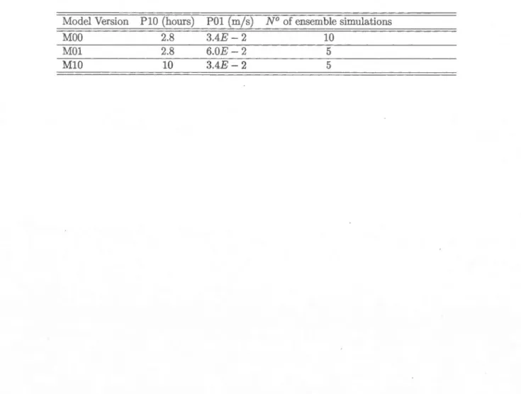
1.1 Parameters' settings used in different model versions. PlO is the time scale of conversion from cloud to precipitable water in the large-scale con-densation parameterization; POl denotes the large-scale vertical velocity threshold in the Kain-Fritsch deep convection trigger function. Model version MOO is used as reference. . . . . . . . . . . . . . . . . 49 2.1 The large-scale vertical velocity threshold in the Kain-Fritsch deep
con-vection trigger function used in the two model versions. Also show is the number of ensemble members . . . . . . . . . . . . . . . . . . 103
AGCM AMIP CGCM CO RD EX CRCM ERA-40 GHG LBC MYNA MYSN NARCCAP PIRCS PRUDENCE RCM RPN SN SYNA SYSN SYDS UKCP LIST OF ACRONYMS
Atmospheric General Circulation Model Atmospheric Model Intercomparison Project Coupled Global Climate Model
COordinated Regional climate Downscaling Experiment Canadian Regional Climate Model
European Centre for Medium-range Weather Forecasts 40-year re-analysis data
Greenhouse Cases
Lateral Boundary Conditions Multi-Year North America Multi-Year Spectral Nudging
North American Regional Climate Change Assessment Program Project to Intercompare Regional Climate Simulations
Prediction of Regional scenarios and Uncertainties for Defining EuropeaN Climate change risks and Effects
Regional Climate Model
Recherche en Prévision Numérique Spectral udging
Single-Year North America Single-Year Spectral Nudging Single-Year Domain Size
-- - - -- - - -- - - - -- - - ---,
RÉSUMÉ
Cette thèse vise à rechercher les configurations expérimentales optimales pour étudier la réponse des Modèles Régionaux du Climat à aire limitée (MRC) face à des perturbations de leurs paramètres. Le travail est présenté en deux parties.
La première partie aborde le cas d'une comparaison entre les simulations provenant d'un MRC, où un événement météorologique ou saisonnier est mis à l'échelle dynamique-ment à partir de données observées (réanalyses). Cette situation implique l'utilisation de périodes d'intégration relativement courtes. Par conséquent, la réponse obtenue dans les moyennes temporelles des simulations par rapport à des modifications aux paramètres a tendance à être noyée dans le bruit quasi-aléatoire provenant de la dynamique chao-tique du MRC. La possibilité d'augmenter le rapport signal-bruit par l'application du pilotage spectral ou par une réduction de la taille du domaine est étudiée. L'approche adoptée consiste à analyser la sensibilité des moyennes saisonnières du MRC Canadien (MRCC) face à des perturbations sur deux paramètres variés un à un. Le premier contrôle la convection profonde tandis que le second régit la condensation stratiforme. Les résultats montrent que l'ampleur du bruit diminue avec la r 'duction de la taille du domaine ainsi que par l'application du pilotage spectral. Toutefois, la réduction de la taille du domaine produit aussi des altérations statistiquement significatives de certains signaux, ce qui favorise l'utilisation de pilotage spectral.
La deuxième partie de cette thèse aborde le cas d'une comparaison entre deux simulations d'un MRC en termes du climat simulé. À cet effet, un cadre théorique est développé pour le calcul des statistiques de premier et second ordre sur la différence entre les simulations. Les statistiques de la différence sont décomposées en une com-posante déterministe et reproductible contrainte par les conditions aux frontières et m1e composante de bruit provenant de la dynamique interne du MRC. Certaines questions reliées à l'estimation de la différence des moyennes temporelles entre les simulations sont développées en détail. Par exemple, un partage optimal des ressources informa-tiques entre la taille d'un ensemble et la longueur de la période d'intégration, ou encore l'impact de la taille du domaine et du pilotage spectral sur l'estimation de la réponse du modèle. Une application de ces considérations théoriques est illustrée à partir de la réponse des simulations du MRCC dont un paramétre lié à la convection profonde a été perturbé.
Mots-clés: modèle régional de climat, perturbation des paramètres, ensemble, com-posante reproductible, pilotage spectral, taille du domaine, différence de moyennes.
ABSTRACT
This thesis aims at finding experimental setups and simulation configurations that facilitate studies devoted to quantifying limited-area Regional Climate Model (RCM) response to parameter modification. The work presented in this thesis is divided in two parts.
The first part addresses the case when the researcher attempts to compare the RCM simulations in tenns of downscaling a particular weather event or season from the objective analyses. This case implies the use of short integration times, and the response of the time-averaged variables to RCM modification tends to be blurred by the quasi-random noise originating in the RCM chaotic dynamics. The possibility of enhancing the signal-to-noise ratio by the application of spectral nudging or domain-size reduction is studied. The approach adopted to study these issues consists in the analysis of the sensitivity of the Canadian RCM (CRCM) seasonal average. to perturbations of two parameters controlling deep convection and stratiform condensation, perturbed one at a time. Results show that the noise magnitude is decreased both by reduction of domain size and the spectral nudging. However, the reduction of domain size produced statistically significant alterations of sorne sensitivity signais, which fosters the use of spectral nudging.
The second part of this thesis addresses the case of comparing two RCM sim-ulations in terms of the simulated climate. For this purpose a theoretical framework is developed for calculation of the first- and second-moment statistics of the difference between RCM simulations, such as time means and variances. The statistics of the difference are decomposed into their deterministic, reproducible components, forced by the boundary conditions, and the quasi-random noise originating from RCM internai dynamics. Sorne issues related to the estimation of the difference of means betwcen control and modified RCM simulations are elaborated in detail, such as the optimal al-location of computational resources between ensemble size and integration time, as well as the impact of spectral nudging and domain size on mean model response estimation. An application of the present theoretical considerations is illustrated by considering the response of CRCM decadal simulations to a perturbation of a deep-convection param-eter.
Keywords: Regional climate model, parameter perturbation, ensemble, reproducible component, spectral nudging, domain size, difference of means.
- - -- - -
-INTRODUCTION
Climate modeling at regional scale
Climate simulations and projections of the future climate at local scale are obtained by coupling separate complex modeling systems. Models of future emission scenarios of greenhouse gases (GHG) and aerosols (Nakicenovic et al. 2000) provide the radiative forcing component in Coupled Global Climate Mo dels ( CGCMs) that are the most com-prehensive tools for climate studies. CGCMs are comprised of the Atmospheric Global Circulation Models ( AGCMs) coup led with the ocean, sea ice and land surface ( e.g., Collins ct al. 2001). Because of their high complexity and the need to perform very long simulation to stabilize the deep ocean, CGCM simulations are very demanding in computational resources and are performed at relatively coarse horizontal resolution. Development of the adaptation and mitigation strategies require information on spatial scales smaller than those provided by CGCMs.
Regional Climate Mo dels (RCMs) are employed to dynamically downscale CGCM simulations to scales of a few tcns of kilometers, using high-resolution representation of the atmospheric dynamics and physics, as weil as forcing at the interface between the atmosphere and the other components of the climate system, only over a specified area of the globe. Different approaches to RCM dynamical downscaling have been developed ( see, e.g., La prise 2008, for a review). So far, the most popular strategy has been the one-way nesting based on high-resolution limited-area RCMs. These models are specifie because they require prescribed information at the lateral boundaries of their computa-tional domain, with no feedback from the nested model to the driving fields ( e.g., Giorgi and Mearns 1999, Rummukainen 2010) .
Climate projections are inherently uncertain because of the fundamental proper-ties of both the elima te system and modeling tools. Sin ce the wor k of Lorenz ( 1963), i t has been acknowledged that due to non-linear chaotic nature of the atmospheric flow, madel solutions are unstable with respect to very small perturbations, so that slight
differences in initial states evolve in time into large differences. This phenomenon has been referred to as intemal variability. Uncertainties associated with constructing and applying the mo dels are manifold. They can be grouped into: (a) structural, (b) pa-rameterization and (c) parameter uncertainties (Murphy et al. 2007). The structural un certain ti es originate iu the choices related to model structure and configuration ( e.g., choices related to grid, resolution, truncation, numerical integration scheme, the set of processes included). Fine-scale physical processes cannot be resolved explicitly in mod-els due to their high complexity and insufficient resolution, and their bulk effect upon the response of the resolved scales is parameterized. The parameterization uncertainties are related to the fuudamental assumptions in the representation of physical processes. Finally, not all parameters that figure in parameterizations can be inferred from first principles of physics or physical experimentation. They may rely on mixture of th eo-retical understanding and empirical fitting, or may even have no counterpart in the real climate system. The uncertainty, thus, also originates in the presence of a large number of adjustable parameters.
Representing uncertainty in climate modeling
In studies with CGCMs, the uncertainty related to model structure and configura-tion has been quantified, as initially proposed in Ri.iisi.inen and Palmer (2001), using multi-model ensembles obtained by combining operational models developed at diffe r-ent research centers. The rationale behind this method lies in the fact that the models grouped in such a way are validated against a large number of observables ( e.g., Giorgi and Mearns 2002, 2003; Tebaldi et al. 2005). The operational models are carefully s tud-ied and they employ different discretization techniques and include different parame -terizations of subgrid processes and other components from a large pool of alternatives (Murphy et al. 2007). However, the method is sometimes criticized for not allowing for an adequate sampling of all possible choices in constructing models, as the models fm·ming multi-model ensembles are assembled on an opportunity basis. The exchange of knowledge between different modeling centers may result in common deficiencies among members of a multi-model en ·emble (Tebaldi and Knutti 2007). In addition, it is not clear how to define a space of all possible model configurations of which the members of a multi-model ensemble would be a sample (Murphy et al. 2007).
3
An alternative approach, based on exploring the uncertain values of adjustable physics parameters in CGCMs has been also developed, mainly as a part of the cli-mateprediction. net project ( e.g., Murphy et al. 2004, Frame et al. 2005, Piani et al. 2005, Stainforth et al. 2005, Barnett et al. 2006, Forest et al. 2006, Knutti et al. 2006, Sanderson et al. 2008, Ackerley et al. 2009). In this approach, the selection of pa-rameters to perturb and estimation of their range of variation are typically conducted by consulting experts that participated in model development. At least in principle, the perturbed-physics ensembles allow for a systematic sampling of related parameter uncertainties and hence afford a greater control of the experimental design than the multi-model ensembles. The perturbed-physics ensemble approach however does not sample uncertainty arising from all choices that must be made among existing options in order to construct a model, such as those related to model structure, configuration, physical processes included or schemes to parameterize these processes. Despite that, it has been shown that the perturbed-physics CGCM ensembles typically exhibit a spread of members as large as the spread in ensembles of different models collected on the basis of opportunity (Murphy et al., 2004, 2007). The perturbed-physics approach has been sometimes criticized because not all the members of a perturbed-physics ensemble can be expected to offer credible climate simulations, as is the case with multi-model ensembles; some of the members may exhibit substantial departures from the observed climate (Stainforth et al. 2005).
The RCMs are specifie because they inherit uncertainty of the driving fields through the lateral boundary conditions (LBC) (e.g., de Elia et al. 2008). There are also specifie choices that must be made in configuring RCM simulations, such as the size and position of the computational domain and the nesting technique, which are also sources of uncertainty. Last but not least, similarly to CGCMs, uncertainty in RCMs also originates in the choices related to their structure, parameterization of sub-grid processes and the adjustable parameters. Multi-RCM ensembles have been increas-ingly employed to quantify the structurallmcertainty in RCMs; there has been a large number of internationally coordinated multi-model experiments designed to address un-certainty specifically in RCM integrations (e.g., PIRCS, Takle et al. 1999; PRUDENCE, Christensen et al. 2007; UKCP, Murphy et al. 2007; NARCCAP, Mearns et al. 2009); CORDEX, (Giorgi et al. 2009). On the other hand, the perturbed-physics ensemble approach to quantifying uncertainty in regional climate began to emerge only recently (e.g., Burke et al. 2010). There were, however, a few early attempts to test RCM
sensi-tivity to structural differences, also including perturbations of physics parameters. For example, Yang and Arritt (2002) and Arritt et al. (2004) showed that the differences between RCMs developed at different centers were much lm·ger than the RCM response to perturbations of parameters. This favored multi-model ensembles as a more efficient technique of sampling differences between RCMs. However, the aforementioned studies examined the RCM response to perturbations of only two parameters in a specifie part of model parameterization, the convective cloud parameterization, which constitutes only a small subspace of a high-dimensional space of adjustable parameters in RCMs.
The main reason why the RCM parameter space remains largely unexplored lies in the fact that, due to a large number of parameters, a thorough ampling of even a small fraction of the parameter space imposes the need for very large computing re-sources that are out of reach for the majority of research centers. Quantifying parameter uncertainty in regional modeling necessitates the use of distributed computing network, such as that adopted by the climateprediction. net. Due to the large number of variable paramet rs, it is impossible to run the model for their every plausible combination and to examine all possible skill scores. In addition, a high skill score does not guarantee that it is achieved for the right reasons, since a high skill can be also a consequence of the cancclation of errors. Furthermore cancelation of errors in simulating the present climate does not imply cancelation of errors in simulating a different climate; there may exist several separated regions of the parameter space in which the model can exhibit a relatively good performance in simulating the observed climate, but yield a consider-able difference in the projected climate change. Renee, a systematic sampling of model response to parameter perturbations may help to improve the parameters settings, as well as to inform about the uncertainty in the projected climate.
Because of the need to procluce more realistic simulations using physically compre-hensive models, the increase in computing speed is usually absorbee[ by adding complex-ity and increasing resolution rather than by an extensive testing of plausible alternatives in applying and constructing the moclels. The increasing complexity of models ham pers their extensive testing, because of an immense number of combinations of adjustable parameters. Another but not less important difficulty is that the estimation of mod 1 response to a modification requires that the signal of moclel response be clistinguishecl from the noise of internal variability of the mocleling system. The most appropriate way to increase the statistical significance of the signal is to devote a sufficiently large
5
computing time to the climate simulations in order to provide a sufficiently large samplc of model states from which robust estimates of the signal can be computed. However, it is typically not possible to generate sufficiently large samples due to the lack of compu-tational resources. The alternative is to employ RCM simulation set-ups that use less computation time. In RCMs this can be done in different ways, which is considered next.
Optimal simulation setup for RCM parametcr modification
The following equation illustrates the classical choices that the numerical modeler must confront when conducting an RCM study:
NxAxHxKxC S
.6.x2 x .6.h ex L x ' (1)
where N represents the number of experiments, A the area covered by the grid, H the total vertical height, K the integration period, C an index of model complexity, .6.h vertical resolution, and .6.x horizontal resolution. On the right-hand side, S rep-resents computer speed, and L the length of project. Computer speed typically does not evolve much during the lifetime of a project and the length of a project is normally non-negotiable and, at best, limited to a few years. The experimental setup is bounded by these two constraints. In or der to increase the number of experiments N, a trade-off has to be made among the other factors on the left hand side of Eq. (1).
The options of reducing model complexity or resolution have been ruled out in this study. Reducing model complexity in order to increase N would considerably change the model structure and make the results very difficult to extrapolate to the operational RCM runs. Changing the horizontal and vertical resolution may also involve issues such as, for example, that the parameter settings in parameterizations of sub-grid processes may be ttmed for the specifie resolution used in the operational RCM runs. This work rather focuses on the possibility of reducing domain size A and the integration period K, in or der to increase the project capacity with respect to the number of modifications N that can be explored. It is important to note that an optimal simulation setup in terms of A and K may not exist. Each setup may require tha~ specifie compromises be made with respect to the potential of extrapolating the results to the typical operational RCM continental-scale domains and multi-decadal rw1s. In the following we discuss the compromises in that respect.
An obvious compromise related to the reduction of the computational area is a loss of generality of the results, since they are confined to a small region of interest. Model response to parameter modification may be very difficult to extrapolate to the geographical regions outside the tested domain, due to different properties of land sur-face or large-scale atmospheric dynamics. There are also other potential issues with the small RCM domains. For example, Leduc and Laprise (2009) provided evidence that the use of small domains can yield RCM simulations deficient in the fine-scale features when compared to the RCM runs conducted in large, continental-scale domains. This problem raises the concern that model sensitivity to parameter modification can be al-tered in different ways in small domains, due to the proximity of the lateral boundaries. On the other hand, when large domains are used, the RCM interior large-scale flow is prone to intermittent inconsistencies with the driving large-scale flow, which may result in large spurious gradients at the perimeter of the lateral boundaries ( e.g., von Storch et al. 2000). The use of small domains can rcduce such incon~istencies.
Reduction of the integration period involves issues related to model internal vari-ability. Because of the chaotic nature of the models and the atmosphere, a negligibly small difference in the initial state eventually yields a large difference in the trajectory in the model phase space. Experiments with climate models point to the fact that the spread between identical integrations that depart from slightly different initial states clecreases upon averaging intime and eventually become small when the averaging time is large (e.g., Giorgi and Francisco 2000, de Ella et al. 2008). The internal variability is triggerecl by any modification in the moclel, regardless of its magnitude and origin (Giorgi and Bi 2000). This implies that any parameter modification woulcl always pro-duce a change in the evolution of the moclel states. If the modification is infinitesimally small, the only response will be the noise of internal variability which is filterecl by averaging in time. So, in the case of an infinitesimally small modification, such as the perturbation in the initial conditions, the differences in the climate statistics clue to the modification are expectecl to be vanishingly small if the integration time is sufficiently large. If the modification is large however, then it may procluce a change in the climate statistics, regardless of the integration time. Renee, in orcier to clistinguish the signal of moclel response to a modification from the internal variability noise in th climate statistics, lm·ger samples of moclel states are needed. It follows from these considera-tions that if the integration period is too short it may be not possible to decide whether
7
the difference obtained between the time statistics of a control and paramcter-modified RCM run is a consequence of the parameter modification or only an apparent difference due to residuals of internal variability. In statistical terminology, we may say that a reduction of the integration period reduces the statistical significance of the signal.
In principle, performing ensemble integrations instead of making inferences from a single integration can solve the problem of the insufficient sample size due to a re -duced integration period. Ensemble integrations can be performed, for example, by perturbing initial conditions. The advantage of RCMs is that, unlike in CGCMs, the spread of RCM ensemble members is a controllable parameter. Reduction of the size of the computational domain may considerably reduce the inter-member variance (e.g., Alexandru et al. 2007). An alternative approach to reducing the ensemble spread is the internal nudging of the large-scale corn ponents of RCM variables ( usually referred to as spectral nudging; von Storch et al. 2000; Biner et al. 2000). This method has been proposed for reducing the intermittent inconsistencies between the internal RCM flow and the driving fields, and has been also employed to reduce the differences between ensemble members (e.g., Weisse and Feser 2003).
Another important issue related to the reduction of the integration period is the representativeness of results with respect to the simulated temporal variability of climate. If the estimates of model response obtained by ensemble integrations over a relatively short period of time are statistically significant, they are so only for this period of time. That is, the results may be statistically significant for given LBC but little representative for sorne other choice of the LBC. For example, the model response could be different if a different period was chosen from the reanalyses to drive the model. This raises issues such as how much generality of results is lost due to a too short integration period and how the loss of generality depends on the ensemble size and simulation configuration (domain size and nudging). Studying variability in time of the RCM response to parameter modification is not a trivial task, since the time variation of RCM variables is partly enforced by the time variation of the driving fields and partly by the RCM internal dynamics. It is thus of interest to study in a systematic manner how a decrease of internal variability noise by spectral nudging or domain size reduction can affect the temporal variability of the model response to modification.
Objectives and approach
This thesis tries to find optimal RCM simulation set-ups that use less computation time than operational runs while still returning representative results. The overall objective of this work is to analyze RCM response to parameter perturbations with simulation set-ups using different integration periods, mode! do mains and large-scale constraints (spectral nudging) and eventually select the set-up that is the most appropriate for conducting a large number of RCM sensitivity tests in a computationally efficient way. The study is conducted in two parts and is presented in form of scientific papers.
In the first part (Chapter 1) the focus is placed on short RCM ensemble integra-tions, conducted over a single year. The goal is to find simulation configurations that maximize the statistical significance of the response of seasonal-average RCM variables but are not detrimental to the response. The approach followed consists in the study of the sensitivity of RCM-simulated seasonal averages to perturbations of two parame-ters controlling deep convection and stratiform condensation, perturbed one at a time. These parameters were selected because they directly influence the formation of precip-itation; this variable represents, along with surface air temperatures, the most relevant variable for climate studies. The both parameters also control the atmospheric liquid and solid water content and bence indirectly affect the surface radiative budget and surface temperatures. In addition, the plausible perturbations of these two parameters produce a relatively large signal in precipitation and surface air temperature, which allows for extracting the signal of model response to perturbations among the noise of interna! variability at a reasonable computing cost.
The sensitivity to perturbations of the deep-convection and stratiform-condensation parameters is analyzed within three simulation configurations: (a) in a large, continental-scale domain, (b) the same domain as in (a) but with spectral nudging, and ( c) in a small domain. In order to sample the contribution of the interna! variability noise to model response to parameter modification, for every setting of these parameters, mul-tiple integrations with perturbed initial conditions are also performed. Signal-to-noise ratio is then studied as a function of the three simulation configurations, which allows for quantifying the reduction in the computational cost by spectral nudging and domain size reduction. In addition, we quantify the alterations of the model response to param-eter modification (signal) triggered by these noise-reducing methods. Optimally, a noise
9
reducing method should efficiently reduce the noise but, at the same time, minimally interfere with the signal.
In the first part of this thesis only the RCM integrations performed over a single year are studied and thus the variability of madel response to parameter modification in time is neglected. The purpose of the second part of this thesis is to examine how much the results obtained in the single-year study depend on the choice of the simulated year. How the spectral nudging and domain size reduction affect this dependence? It turns out that this is a rather complex issue that requires a specifie theoretical framework. Chapter 2 first presents a general theoretical framework for studying temporal variab il-ity of RCM response to modification. The theoretical considerations are then employed to analyze perturbed-parameter RCM simulations conducted over a 10-year integration period in different RCM simulations configurations.
CHAPTERI
IMPACT OF SPECTRAL NUDGING AND DOMAIN SIZE IN STUDIES OF RCM RESPONSE TO PARAMETER MODIFICATION
This chapter is presented in the format of a scientific article. It was submitted to the jomnal Climate Dynamics and is now published. The manuscript is entirely based on my work, with the co-authors involved in interpretation of the results and text editing. The detailed reference is:
Separovic, L., de Elia R. and Laprise, R., 2011: Impact of spectral nudging and domain size in studies of RCM response to parameter modification. Climate Dynamics, doi: 10.1007/ 00382-011-1072-7
Impact of Spectral Nudging and Domain Size in Studies of RCM Response to Parameter Modification
Leo Separovic, Ramon de Elia and René Laprise
Leo Separovic - René Laprise
Centre ESCER (Étude et Simulation du Climat à 1 Échelle Régionale), Département des Sciences de la Terre et de 1' Atmosphère
Université du Québec à Montréal (UQAM) B.P. 8888, Suce. Centre-ville
Montréal (Québec) Canada H3C 3P8 Ramon de Elia
Centre ESCER (Étude et Simulation du Climat à 1 Échelle Régionale), Consortium Ouranos, 550 Sherbrooke West,
13
Abstract
The paper aims at finding an RCM configuration that facilitates studies devoted to quantifying RCM response to parameter modification. When using short integration times, the response of the time-averaged variables to RCM modification tend to be blurred by the noise originating in the lack of predictability of the instantaneous at-mospheric states. Two ways of enhancing the signal-to-noise ratio are studied in this work: spectral nudging and reduction of the computational domain size. The approach followed consists in the analysis of the sensitivity of RCM-simulated seasonal averages to perturbations of two parameters controlling deep convection and stratiform conden-sation, perturbed one at a time. Sensitivity is analyzed within different simulation configurations obtained by varying domain size and using the spectral nudging option. For each combination of these factors multiple members of identical simulations that differ exclusively in initial conditions are also generated to provide robust estimates of the sensitivities (the signal) and sample the noise. Results show that the noise magni-tude is decreased both by reduction of domain size and the spectral nudging. However, the reduction of domain size alters sorne sensitivity signals. When spectral nudging is used significant alterations of the signal are not found.
Key words: Regional climate models, parameter perturbations, internal variability, spec-tral nudging, domain size
1.1 Introduction
Nested limited-area Regional Climate Models (RCMs) are models that dynamically downscale global General Circulation Model (GCM) simulations or objective analyses to high-resolution computational grids, using a high-resolution representation of the surface forcing and model dynamics. RCMs require the information on some prognostic variables as their lateral boundary conditions (LBC). The choices of integration do-mains and nesting techniques are free parameters of RCMs. The optimal integration domain depends on the particular situation, although there are some general recom-mendations that can facilitate users judgment (e.g., Laprise et al. 2008). For example, Leduc and Laprise (2009) showed that the use of a too small domain could result in the simulations being deficient in fine-scale variance. It has been also noted that in large continental-scale domains RCM large-scale variables can considerably drift from the driving fields, which can then result in appearance of large spurious gradients in the vicinity of the outfl.ow boundaries. Spectral nudging (SN; von Storch et al. 2000; Biner et al. 2000) has been employed to erlSure that the model solution remains close to the large-scale components of the driving fields over the entire domain. However, the use of SN remains an open issue. Alexandru et al. (2009) raised concern that the application of the SN could suppress the proper generation of fine-scale features. However, Colin et al. (2010) did not find SN to be detrimental on the modelling of extreme precipitation.
The choice of the integration domain and the use of SN can have a large impact on the RCM internai variability. Internai variability arises due to the non-linear, chaotic nature of atmospheric models: any perturbation; however, small it is in magnitude, provokes the trajectori s of the model solution in the phase space to diverge in time. In autonomous Global Circulation Models (GCMs) the difference between two simulations conducted with the same model but departing from initially slightly different states is on average as large as the difference between two randomly chosen GCM states, given a specifie season. Internai variability also emcrg s in RCMs but, typically, it is smaller than in GCMs; the advection of information prescribed as the LBC keeps the evolution of the RCM internai variability somewhat bounded ( e.g., Giorgi and Bi 2000, Caya and Biner 2004). However, intermittently in specifie areas of the integration domain it can achievc values as large as in GCMs (Alexandru et al. 2007). Its time evolution appears to depend on the synoptic situation enforced by the driving fields (e.g., Lucas-Picher et al. 2008a; Niki ma and La prise 2011) and is scal selective (Separovic et al. 2008).
15
Reduction of domain size or the application of SN can both considerably reduce internai variability in RCMs (Alexandru et al. 2009). Thus, the average amplitude of internai chaotic variations appears to be in RCMs, to a certain extent, a controllable parameter. This fact may be of particular interest in studies oriented to RCM testing and mod ifi-cation.
The sensitivity of a RCM to any change in its structure and configuration, such as a modified parameterization or a perturbation of its tuneable parameters, generally consists of the response of the simulated variables to the modification (sig·nal), as well as of internai variability noise. Since the work of Weisse et al. (2000) it has been widely acknowledgcd that estimation of the signal in the temporal evolution of the RCM vari-ables requires ensemble simulations that can be generated, for example, by imposing perturbations to the initial conditions of bath the control and the modified madel ver-sions. Internai variability deviations are partly filtered in the ensemble mean depending on the ensemble size, as the variance of the samplc mean of a collection of independent and identically distributed random variables is inversely proportional to the sample size (e.g., von Storch and Zwiers 2002). When the signal is small or the internai variability is large, ensembles of large size are needed in arder to obtain statistically significant estimates of the simulation differences resulting from the madel modifications. For suf-ficiently long integration times, internai variability deviations are substantially reduced in the time average. However, estimation of the time averages computed over shorter periods from years to a decade also necessitates sampling of the internai variability de-viations, since it can be still non-negligible in the time average of the single madel run, especially for fine-scale variables such as precipitation (de Elia et al., 2008; Lucas-Picher et al., 2008a, b). When considering the difference ·between the time a ver ages in the con-trol and a modified model version, the variance introduced by the internai variability is twice as large as that in the time average in each madel version, due to the aggregation of error through the difference tenns.
Providing statistically significant estimates by means of ensemble simulations or longer integration periods for the control and modified madel versions is bence compu-tationally time consuming. While this issue might be of little relevance when the RCM is to be tested for a single modification, it can represent a hindrance in studies that require multiple testing of RCM response to modifications of a large number of param-eters. This would typically be the situation in deliberate madel tuning or in studies
that address uncertainty originating in the RCMs adjustable parameters wherein it is essential to identify in a high-dimensional parameter space the plausible parameter per-turbations that produce th largest response of the model (e.g., Sexton and Murphy 2003). The underlying methodological issue in such RCM studies is thus to optimize the use of computational resources by finding an appropriate test bed configuration (prototype simulation) that would be as inexpensive as possible in terms of the number of computational points and integration time and that can provide robust estimates of the model response to the modifications.
Our working hypothesis is that suppressing the internai RCM variability by means of domain size reduction or application of SN woulcl allow for quantifying the signal with a smaller ensemble size and help to recluce the computational cost (Alexandru et al. 2007, Weisse and Feser 2003). The application of these methods to reduce internal variability noise requires better understanding of the ways they might alter the signal of RCM sensitivity to modification, e.g., by suppressing its magnitude. Too small domains are generally non-recommended for climate simulations and sensitivity studies because of the spurious effects of the proximity of the lateral boundaries, fine-scale variance defi-ciency and lack of continental-scale interactions and feedback among the RCM variables (e.g., Jones et al. 1995; Seth and Giorgi 1998; Laprise et al. 2008). Results obtained in such domains are likely to be less realistic and difficult to extrapolate to the operational RCM simulations. However, when studying uncertainties originated in adjustable RCM parameters, a very large number of tests are required and the user may wish to conduct preliminary tests in a computationally inexpensive small domain. Outside this context the reduction of domain size and SN should not be considered as competing techniqu s to improve the signal-ta-noise ratio since the SN has not been shown to involve similar difficulties.
The manuscript is organized as follows. The model and the modifications per-formecl on the model parameters in orcier to produce modified modcl versions and the experiments are described in Section 2. The analysis of model sensitivity to modifica-tion of parameters within different simulation configurations is carried out in Section 3. Summary and conclusions are provided in Section 4.
- - - -- - - -- - -
-17
1. 2 Experimental design 1.2.1 Model description
The model used in this study is the fifth-generation Canadian Regional Climate Model (CRCM5; Zadra et al. 2008). It is a limited-area version of the Canadian weather forecast model GEM (Côté et al. 1998); the model has a non-hydrostatic option, a l-though this feature is not exploited here. GEM is a grid-point model based on a two-time-level semi-Lagrangian, semi-implicit time discretization scheme. The model includes a terrain-following vertical coordinate based on hydrostatic pressure (Laprise 1992) with 58 levels in the vertical, and the horizontal di ·cretization on an Arakawa C grid (Arakawa and Lamb 1977) on a rotated latitude-longitude grid with a horizontal resolution of approximately 55 km and time step of 30 min. The nesting technique employed in CRCM5 is derived from Davies (1976); it includes a graduai relaxation of all prognostic atmospheric variables toward the driving data in a 10-point sponge zone along the lateral boundaries. The lateral boundary conditions (as well as the initial conditions) are derived from ERA40 reanalysis (Uppala et al. 2005). Ocean surface conditions are prescribed from Atmospheric Model Intercomparison Project (AMIP) data (Taylor et al. 2000).
1.2.2 Experiments
Modified model versions are obtained by perturbing the CRCM5 physics parameters. Three different mo del versions are considered: the control version ( denoted hereafter as MOO) and two perturbed-parameter versions ( denoted by MOl and MlO) obtained by perturbing one at a time, the following two parameters:
POl - Threshold vertical velocity in the trigger function of the deep convection parameterization (Kain and Fritsch 1990).
PlO- Cloud water to precipitation conversion time scale in the large-scale conde n-sation parameterization for stratiform precipitation (Sundqvist et al. 1989; Pudykiewicz et al. 1992).
The values of parameters used in the three model versions are given in Table 1.1. Two experts that participated in CRCM5 development judged the perturbations as being moderate to strong with respect to their range of variation, given the ho
ri-zontal resolution (B. Dugas and P. Vaillancourt, both from Environment Canada RPN, personal communication).
Three sets of experiments are carried out in this study, all based on simula-tions conducted over a single year. For every model version multiple perturbed initial-condition ensemble simulations were performed. The initial conditions were perturbed initializing the model from November 01 1992 at OOUTC onward, 24 h apart. All the simulations, regardless of model version and initialization time, end on December 01 1993 at OOUTC. November 1992 is not considered in order to allow the spin-up of the initial differences, thus leaving a 1-year period for the analysis. The number of ensemble members is the same in all three sets; there are 10 members for the standard model version MOO and 5 members per each of the two perturbed-parameter versions MOl and MlO (see Appendix 1.5 for more details); the last column in Table 1.1 shows the ensemble size per each model version.
In the first set, denoted as SYNA, the simulations were performed with the three model versions (MOO, MOl and MlO) over the large continental-scale domain, referred to as NA, consisting of 1202 grid points, and shown in Fig. L 1 including the lü-point relaxation zone at the perimeter of the lateral boundaries.
The second set of experiments, denoted as SYSN, is identical to SYNA in terms of its domain (NA; Fig. Ll), model versions and number of ensemble members per every mo del version (Table L 1); the only difference is that the SN was used. The nudging was only applied to the horizontal wind components, with the truncation at non-dimensional wavenumber 4 (1, 500 km). The SN strength is set to zero below the level of 500 hPa and increases linearly with height, reaching 10% of the amplitude of the driving fields per time step at the top leveL The choices of the truncation wavelength and the vertical profile of the nudging strength refiect the intention not to interfere with the model own interior dynamics at fine and intermediate spatial scales and in the lower half of the model's atmosphere.
The third set of experiments, denoted as SYDS, consists in reducing the domain size. For every model version, the single-year ensemble simulations are generated again, but over a domain of reduced size centred over the province of Quebec (without SN).
19
The domain for the SYDS experiment consists of 702 grid points and is shown in Fig. 1.1, including the lü-point sponge zone.
1.3 Results
The variables selected for the analysis of results are seasonal-average precipitation and 2 rn-temperature. The analysis is focused on the influence of SN and domain size reduction on the model sensitivity to perturbations, internai variability noise and sig11al-to-noise
ratio. This section is organized as follows. Section 1.3.1 briefly reviews the sensitivities of CRCM5 seasonal averages to perturbations of the initial conditions and parameters, as a function of season and experimental configurations SYNA, SYSN and SYDS. S ec-tion 1.3.2 presents the spatial distribution of the internai variability noise in the three configurations. Sections 1.3.3 to 1.3.5 examine the spatial patterns of the sensitivity of CRCM5 seasonal averages to the parameter perturbations (signais), estimated with the difference of ensemble means of the control and modified model versions; these sec -tions also provide the statistical significance of the sensitivity estimates and compare the signal patterns in the three simulation configurations. Section 1.3.6 examines the computational cost associated with different simulation configurations in terms of the minimum ensemble size necessary to achieve significant estimates.
1.3.1 Spread of differences excited by perturbations
We begin the analysis with a brief review of the magnitude of the response of the CRCM5 seasonal averages to the applied parameter perturbations, as a function of the simula -tion configuration (SYNA, SYSN and SYDS) and season (DJF, MAM, JJA, and SON). For this purpose the square root of the spatially averaged square differences ( denoted as rmsd) is computed for the pairs of seasonal averages obtained from the simulations that differ either in the parameters settings (signal) or initial conditions (internai var i-ability). The rmsd excited by the perturbations of parameters are calculated using the pairs of seasonal averages, such that each pair consists of one realization of the control ensemble MOO and one realization of the perturbed-parameter ensemble (MOl or MlO). Since the latter have 5 members ( see Table 1.1), 5 pairs were randomly chosen from the 10 members of the reference model, and bence 5 pairs of difference were computed for each parameter perturbation. The rmsd are displayed in Fig. 1.2 with the 5 plus marks
coloured in red for the perturbation of the deep convection parameter and the 5 marks in blue for large-scale condensation parameter, for seasonal-average precipitation (a) and 2 rn-temperature (b). All rmsd are computed for each configuration over its own domain exclusive of the lü-point wide sponge zone; thus in the SYNA and SYSN experiments, the rmsd is computed over the large domain, while for the SYDS over the small domain in Fig. 1.1. Th rmsd displayed with coloured marks in Fig. 1.2 are a result of the model response to the parameter perturbations. Internal variability is displayed with black marks in Fig. 1.2. They represent the rmsd excited by different initial conditions of simulations with otherwise identical model configurations. The rmsd are assessed from the 10 ensemble members of the control model version MOO that are organized in five pairs on a random basis.
Figure 1.2 shows that all rmsd exhibit an annual cycle with the maximum in summer and minimum in winter. The magnitude of the rmsd illustrates the physi-cal significance of the model response to perturbations. The range of responses for precipitation and 2 rn-temperature is 0--0.3 mm/clay and 0-0.7°C in winter and 0.3-0.8 mm/clay and 0.6-l.5°C in summer, r spectively. Also the rmscl are in general the largest in the SYN A set and the smallest in the recluced domain size SYDS set. This holds for the three kinds of perturbations. The SYSN recluces internal variability noise (black marks) but it is less efficient in that than the reduction of domain size (SYDS); this being true for this case and different configurations of both SN and domain size coulcl yield different results. The plots in Fig. 1.2 also provide a rule of thumb for the statisti-cal significance of the response of the seasonal averages to the parameter perturbations: if differences between the control and perturbed-parameter model version (red or blue marks) tend to lie above the maximum rmsd due to internal variability noise (black marks), given. a season and simulation setup, this suggests the statistical significance of the corresponcling moclel response to the parameter perturbation. As of precipitation (Fig. 1.2a), all signal rmsd in the SYNA setup are barely above noise level, except for condensation-related parameter PlO in winter. The SN and reduction of domain size re-duce the noise nnscl considerably but also the nnsd clue to the parameter perturbations generally decreases. Thus, for precipitation in the SYSN and SYDS sets, the situation with statistical significance is not considerably changed. The exception is in summer when the convection-related parameter POl procluces significant rmscl, especially in the SYDS set. For 2 rn-temperature (Fig. 1.2b) the responses to parameter perturbations are generally more tatistically significant. Despite that, when the signal is weak, as
21
POl in winter, or noise very high, as in spring and summer, the parameter-induccd rmsd appear not to be statistically significant. This also implies that the signal-to-noise ratio varies for different CRCM5 variables.
It is difficult to infer from Fig. 1.2 whether the model response to parameter perturbations is on average smaller in the SYSN and SYDS sets or whether the lower rmsd in this set are a sole effect of reducing internai variability. We investigate this issue more thoroughly in the next subsections. Further, it can be seen that in winter (DJF), the perturbation PlO produces considerable and significant signals for both pre-cipitation and temperature, while POl produces a smaller response that is difficult to distinguish from internal variability. Perturbation POl is related to the deep convection parameterization that is rarely active in winter over land. This perturbation produces a considerable and significant response over land only in the warmer half of the year.
The spatially averaged square differences may hide important information on the local behaviour of the CRCM5 response to the perturbations. In the following we begin the analysis of spatial patterns by first examining the noise level and then the spatial patterns of the model response to parameter perturbations are compared in the three experimental sets as a function of the parameter perturbation and season.
1.3.2 Noise level in the differences
Instead of using a standard measure of noise in seasonal a ver ages ( e.g., ensemble stan-dard deviation in the control model MOO) that would quantify the internai variability in CRCM variables, we rather analyze the internai variability of the model responses to the perturbations of parameters. This way, every difference computed between an ensemble member of a perturbed-parameter model (MOl or MlO) and a member of the control model ensemble MOO is a sample of the model response to the parameter perturbation. Internai variability noise in estimates of the CRCM5 response can be measured with the variability in that sample. Since the variance of the difference of the two mutually independent identically distributed (iid) random variables is equal to the sum of the variances of the two variables, the standard deviation of the sample of differences can
be estimated as
(1.1)
where the overbar denotes the time average over a three-month season, the angle brac
k-ets denote the ensemble average, Mx and My denote the number of ensemble realizations
of a CRCM5 variable in the control (x) and a modified model version (y), respectively, and are given in Table 1.1. This specifie rneasure of noise is employed to stress the fact
that the ensemble variance of the difference between the two model versions is equal to the sum of the variances of the control and the modified rnodel ensembles.
The noise measured with the standard deviation (Eq. 1.1) is displayed in Fig. 1.3 for the three single-year sets (SYNA, SYSN and SYDS) as a function of the parameter perturbation, season and CRCM5 variable. It is computed for differences between the
members of the control (x) and a modified MlO version (y); similar patterns are ob-tained when MOl is used instead of MlO (not shown). Note that the same colour bar is used for precipitation and temperature. In winter the noise in precipitation in the
SYNA set (Fig. 1.3a) is rather low in absolute terms, with values up to 0.3 mm/day
over the southeastern portion of the continent and up to 0.7 mm/day off the East Coast of North America. However, these values are considerable in relative terms because the precipitation rates in winter are generally low, especially over the continent. The SN and reduced domain size (Fig. 1.3b, c) help to reduce noise level for precipitation in winter to fairly low values. The patterns of the 2 rn-temperature in winter (Fig. 1.3d-f) are similar to precipitation; noise locally attains 0.6°C over the northern Canada in the SYNA set and is almost entirely suppressed in the SYDS set. However, in summer, the standard deviation of the differences between the control and modified madel versions
attains striking values in the SYNA set. For precipitation (Fig. 1.3g) it locally attains
2.5 mm/day over the southern and eastern coastal regions of the continent. SN (Fig. 1.3h) is not very efficient in reducing noise. The domain size reduction (Fig. 1.3i) re -duces noise but locally it is still up to 0.6 mm/day. As of 2 rn-temperature in summer
(Fig. 1.3j-l), noise levels are barely higher than 1 °C. SN suppresses the noise below 0.6°C and the reduction of domain size below 0.2°C.
23
studying RCM response to modification using single-year simulations. It is not likely that any reasonable modification performed on the state-of-the art RCMs would produce lar·ger differences in summer precipitation than the values of the noise-induced standard deviation of the differences displayed in Fig. 1.3g. This implies a relative error of 100% in the estimates of the CRCM5 sensitivity to the parameter perturbations obtained without ensemble integrations. Time averaging over a season is not sufficient to ensure filtering of internal variability noise, and averaging over an ensemble or a longer period is required to assess the signal.
1.3.3 Signal PlO in winter
In this subsection we examine the change in seasonal averages due to the perturbation in the large-scale condensation parameter PlO (Table 1.1). As before, we denote the CRCM5 variable obtained in an individual simulation in the control model ensemble MOO with x and the same variable in the modified model ensemble MlO with y. The change in the CRCM5 seasonal averages due to the perturbation PlO is quantified by the difference of time-average ensemble averages of y and x; the difference is computed in each simtùation setup (SYNA, SYSN and SYDS) and will be referred to as the signal. Because of the internal variability in seasonal averages, especially in summer, and the relatively small number of available ensemble members for the two modified model ver-sions MlO and MOl, the ensemble averages are also prone to the noise-induced sampling error. In order to avoid erroneous interpretation of internal variability residuals in the ensemble averages as the model sensitivity to the parameter perturbations, statistical significance of the responses is also eval uated using the test for differences of means (von Storch and Zwiers 2002). For the pm·pose of testing, the true ensemble variances of the control (x) and modified model version (y) are assumed to be equal, as we believe that the differences between these variances in model versions considered here are reasonably small with respect to the sampling error of their estimates. Under this assumption, the test statistic for the null hypothesis of no difference between the two model versions, is given as
where the overbar denotes seasonal average, the angle brackets ensemble average and Mx (My) are the ensemble sizes corresponding tox and y. The quantity
82 =
~~~1
(flm
-
(Y) ) 2+
~~~
1 (
xm-
(x) )2w Mx+My -2 (1.3)
is the pooled estimation of the ensemble variances of the control and modified model version. Here, Mx = 10 and My = 5, as shown in Table 1.1. The ensemble size of the
control version is doubled in order to increase the signal to noise ratio and to estimate well the ensemble variance for at least one model version. Appendix 1.5 provides a
discussion on how to select the number of ensemble realizations Mx and My in order to optimize the signal-to-noise ratio (Eq. 1.2). Under the null hypothesis of equal means of the two model versions, t follows the Student's distribution with
f
= Mx + My - 2 degrees offreedom (f = 13 here).The model resporise to the perturbation of the large-scale condensation
param-eter PlO (signal), as estimated by the difference of the ensemble means of the model
versions MlO and MOO, is presented in Fig. 1.4a-c for winter-average (DJF) precipita-tion in the SYNA, SYSN and SYDS experimental sets, respectively. The corresponding
fields of statistical significance are shown in Fig. 1.4d-f. The regions of high significance (above the 90% level), corresponding to the positive (negative) values of the signal, are
coloured red (blue). In the SYNA set (Fig. 1.4a) the strongest and also highly si
g-nificant (Fig. 1.4d) signal is aligned with the entire Pacifie Coast. It reaches locally
up to ±2 mm/ day. The signal is negative over the eastern Pacifie Ocean off the West Coast and more precipitation is brought inland over the Rocky Mountains region by
the westerly flow that dominates this area in winter. The imposed perturbation implies that the time scale for conversion of cloud to precipitable water in the parameterization
of the large-scale (stratiform) condensation in the version MlO is longer thau in the reference version MOO. It is worth noting that this perturbation is independent of the parameterization of deep convection in CRCM5 and thus should have no direct effect on
convective precipitation, although indirect effects are possible. Another noticeable f ea-ture in the SYNA set (Fig. 1.4a) is a mainly negative signal over the southeast portion
of the domain, significant at 95% level. Also note that in several regions in Fig. 1.4d
over the central part of the continent the signal is highly significant, but its magnitude is too low to make a fingerprint with the contour interval used in Fig. 1.4a. This