Science Arts & Métiers (SAM)
is an open access repository that collects the work of Arts et Métiers Institute of
Technology researchers and makes it freely available over the web where possible.
This is an author-deposited version published in:
https://sam.ensam.eu
Handle ID: .
http://hdl.handle.net/10985/17207
To cite this version :
Stéphane CHEVALIER, Jean-Christophe OLIVIER, Christophe JOSSET, AUVITY - Polymer
electrolyte membrane fuel cell operating in stoichiometric regime Journal of Power Sources
-Vol. 440, p.227100 - 2019
https://doi.org/10.1016/j.jpowsour.2019.227100
Received 4 July 2019; Received in revised form 28 August 2019; Accepted 1 September 2019 0378-7753/
Polymer electrolyte membrane fuel cell operating in stoichiometric regime
S. Chevalier
a,*, J.-C. Olivier
b, C. Josset
c, B. Auvity
caI2M - Institut de M�ecanique et d’Ing�enierie de Bordeaux (CNRS UMR 5295) �Ecole Nationale Sup�erieure d’Arts et M�etiers (ENSAM), Esplanade des Arts et M�etiers,
33405, Talence C�edex, France
bIREENA Laboratory (EA 4642), Universit�e de Nantes, 37 boulevard de l’universit�e, BP 406, 44602, Saint-Nazaire Cedex, Saint-Nazaire, France
cLaboratoire de Thermique et �Energie de Nantes (CNRS UMR 6607), Polytech Nantes, Universit�e de Nantes, La Chantrerie, rue Christian Pauc - CS 50609, 44306,
Nantes Cedex 3, France
H I G H L I G H T S
�Fuel cell stoichiometric regime is evidenced at global and local scale.
�Cathode channel mass transport governs the fuel cell performance in this regime. �Low frequency spectral signature of stoichiometric regime is measured using EIS. �Current density distributions are measured using a segmented flow field. �Fuel cell kinetic parameters can be easily measured in stoichiometric regime.
A R T I C L E I N F O Keywords:
Stoichiometric regime Analytical model Segmented cell PEM fuel cell EIS
A B S T R A C T
In this work, we report the existence of a stoichiometric regime where the performances of operating polymer electrolyte membrane (PEM) fuel cells are entirely governed by the mass transport in the cathode channels. An analytical model of the fuel cell stoichiometric regime is derived and evidenced experimentally: from the cell spectral signature at low frequency based on electrochemical impedance spectroscopy, and from the current density distribution measured using a segmented current collector. The existence of such regime provides a simple way to characterize, model and predict PEM fuel cell performances.
1. Introduction
Alternative engines to convert and store energy which do not pro-duce any greenhouse gas are a must need. Among the large variety of processes such as wind turbine or solar panel for example, Polymer Electrolyte Membrane (PEM) fuel cells are one of the most promising candidates. They convert hydrogen and air into electricity and heat with water as the only by-product. The efficiency of the direct conversion of the chemical energy into electrical energy is also an important asset of this technology. Today, PEM fuel cells are close to the commercializa-tion, but their cost still needs to be decreased to reach the full market deployment [1,2]. To make the fuel cells less costly, one way is to in-crease the electrical power density for a given cell. This can be achieved by both improving the electrochemistry [3] and the mass transport in all the fuel cell materials [4].
To study and improve the mass transport in fuel cells, numerous numerical models have been developed by the research community from
the cell scale to the pore scale in the GDL or in the catalyst layer [5–7]. Comprehensive reviews of fuel cell mass transport mechanisms are available in the literature [4,8,9] which summarise all the recent ad-vances in fuel cell modeling. An ubiquitous drawback to all the models reported in the previous references is the large number of parameters required (more than ten in general, see Refs. [10,11] for example). If few of them can be easily obtained such as the cell dimensions, or operating conditions, most parameters related to the GDL properties (conductivity, permeability), catalyst layer properties (kinetic reaction coefficients) or PEM properties (drag coefficient [12], ionic conductivity) are – in most cases – not accurately known, which introduce a lot of uncertainty in fuel cell model results. In this context, and to overcome this problem, some authors have developed simplified models which rely onto a very limited sets of fuel cell parameters [13–20]. Such less parametrised models usually work under strong assumptions and over a limited range of operating regimes – which allow for neglecting some of the fuel cell phenomena such as the anode electrochemical reactions for example. In counter part, these simplified models are well suited to make accurate * Corresponding author.
fuel cell properties measurements such as electrochemical properties. Alongside fuel cell model developments, experimental character-izations of fuel cell properties have been widely reported in the litera-ture. These works were focused at different scales: from the system scale where a whole fuel cell stack is studied [21,22], to component scale where the liquid water transport was imaged in the GDL pores via X-rays radiography for example [23–26]. In between, the single fuel cell behaviour was also studied using mainly electrochemical techniques such as Electrochemical Impedance Spectroscopy (EIS) [27]. This technique is particularly well suited to characterize fuel cell kinetics [28], membrane resistance [29] and mass transport in both GDLs and channels [16,30,31]. A comprehensive review of the fuel cell phenom-ena which can be characterized through EIS is given in Ref. [32]. However, EIS applied to the cell gives a global characterization of the physical phenomena whereas it is well admitted that the fuel cell properties can change along the channel [33,34]. Thus, segmented fuel cells were developed in order to measure local current densities [35] and to perform local electrochemical characterizations [33]. Different de-signs of segmented fuel cell were developed, using segmented straight channels [36], serpentine channels [37], or combining segmented fuel cell with optical visualisations [38]. In all the previous works, the great interest of segmented fuel cells was clearly proven to study the local changes of fuel cell current density, water concentration, or temperature.
In authors’ previous works [16], it was shown that a stoichiometric regime can be identified in operating fuel cells. Such regime appears at low to moderate current density (less than 1 A/cm2) when the mass
transport limitations in the GDL can be neglected [15,16,39]. It can be identified using the EIS signature at low frequency (between 3 and 0.5 Hz). It was shown that this low frequency signature is a consequence of the oxygen transport in the channel [40] which is different from the inductive low frequency behavior pointed out by Pivac et al. [41,42] to monitor fuel cell aging. Low frequency capacitive loop can also be observed in case of dehydrated membrane as reported by Chevalier et al. [43], but at frequency lower than 1 Hz and in case of very dry operating conditions. Therefore, low frequency capacitive loop measured at low stoichiometry using relatively well hydrated membrane are likely related to oxygen transport in the channel.
Going further, we extend these previous works [16,39] to the local
scale, where the current density distribution should depend only on the oxygen stoichiometry in the stoichiometric regime [44]. A segmented fuel cell was specially designed to measure the current density distri-butions. Once the stoichiometric regime clearly identified, a method-ology to characterize the fuel cell electrochemical properties (Tafel slope and exchange current density) is derived from the equations of this fuel cell operating regime. These findings answer the need of less para-metrised models for accurate fuel cell properties characterisations and bring two original results compared to the authors’ previous works: (i) the evidence of a stoichiometric regime at the local scale (through current density distribution), and (ii) a methodology to accurately characterize the fuel cell kinetics parameters under the stoichiometric regime.
Subsequently in the paper, what is called the global scale is the cell scale at which the cell impedance is measured. The local scale designates the channel scale at which the segmented current density measurements are performed.
2. Methods
2.1. Current density distribution in the stoichiometric regime
The analytical model used to describe the current density and the low frequency impedance in stoichiometric regime is derived from the au-thors’ previous work [15,16]. It was shown that under the assumption of negligible performance losses at the anode and the absence of liquid water in GDLs and channels, fuel cell models can be reduced to a simplified model governed by three dimensionless parameters. The Wagner number, Wa ¼ b=ðrΩj0Þ, which compares the voltage losses in the CL to the voltage losses in the membrane. The Damkh€oler number, Da ¼ iceðE0 EÞ=bhg=ð4FcrefDeffÞ, which compares the kinetics of the reac-tion to diffusive flux of oxygen in the GDL. And the Peclet number, Pe ¼
uchchg=ðDeffLcÞ, which compares the ratio of oxygen transported in the channel to the mass transport in fuel cell porous media. At low current density and low membrane resistance, the stoichiometric regime exists for a particular set of these parameter values, i.e. when the Wagner number is found to be large enough to neglect the overpotential gradi-ents along the channel in the PEM, and when the Damkh€oler is small enough to neglect the concentration gradient in the GDL, i.e. the oxygen Nomenclature
Parameters and variables
b V, Tafel slope
cc mol/m3, oxygen concentration in the channel
cref mol/m3, Reference concentration at the channel inlet
Da Damkholer number
Deff m2/s, Effective diffusivity of the GDL
Ecell V, Fuel cell potential
F C/mol, Faraday constant
hc m, Channel depth
hg m, GDL thickness
i Complex unity
ic mA/cm2,Exchange current density
Icell A/cm2, Fuel cell current density measured by the FC station
j A/cm2, Local current density
j0 A/cm2, Inlet current density
lc m, Cell width
Lc m, Channel length
M g/mol, Molar mass
Pe Peclet number
_
Q ml/min, Air flow rate in operating pressure and
temperature _
QSCPT ml/min, Air flow rate in standard condition of pressure and
temperature
rHF mΩ, Fuel cell ohmic resistance
R J/mol/K, Ideal gas constant
Rct Ω.cm2, Charge transfer resistance
T K, Temperature
uc m/s, Air velocity
Wa Wagner number
x Molar fraction
y m, Spatial coordinate
Z Ω.cm2, Complex fuel cell impedance
Greek letter
αc Dimensionless charge transfer coefficient
δ Periodic state φ �, Phase η V, Overpotential in the CL λ Oxygen stoichiometry ρ kg/m3, Density τ s, Characteristic time ω rad/s, Angular frequency
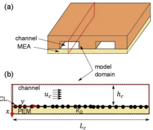
concentration in the CL is equal to the one in the channel. Under these conditions, the fuel cell is assumed to be operating in the stoichiometric regime [6,15,39], and the fuel cell geometry can be simplified as depicted in Fig. 1. Thus, in the stoichiometric regime, the fuel cell can be viewed as a flow field directly in contact with the catalyst layer; the GDL has no impact onto the fuel cell performances since the concentration gradients in the GDL are neglected as well as its ohmic losses.
The other main assumptions of the model concern the transport of liquid water and the value of the fuel cell parameters. In the present model, the liquid water is not explicitly modelled. It is considered that its impact can be seen through the values of the fuel cell parameters, such as the PEM ohmic resistance or the catalyst layer kinetics among others. In addition, fuel cell parameters are considered to be effective values which are constant along the channel (y-direction in Fig. 1(b)). To simplify the calculations and the model, we also consider that the fuel cell is isothermal with ideal current collectors (no ohmic losses in them). The oxygen transport in the channel is assumed to be a plug-flow with an averaged air velocity, uc. In addition, a plane CL is considered at the
cathode, meaning that the electrochemical reaction takes place homo-geneously throughout the CL thickness. This last assumption is valid in case of rapid oxygen and charge transport in the CL [14]. Finally, the present stoichiometric model takes into account only the slowest tran-sient phenomena occurring in fuel cells, i.e. the charging/discharging phenomenon in the double capacity layer is neglected.
Thus, under all these assumptions, a relatively simple expression of the transient current density distribution can be written as:
jðy; tÞ ¼ ic ccðy; tÞ
cref e
ηðtÞ=b; (1)
where j is the current density, ic is the exchange current density, cc is the
oxygen concentration in the channel, η is the overpotential, and b is the
Tafel slope. The transport of the oxygen concentration in the channel is governed as follows: ∂cc ∂t ðy; tÞ þ uc ∂cc ∂yðy; tÞ ¼ jðy; tÞ 4Fhc ; (2)
where uc is the air velocity, F is the Faraday constant and hc stands for
the channel depth. Equations (1) and (2) are rewritten in dimensionless form using the following parameters: j�¼j=j0 where j0¼jð0Þ is the inlet current density, ~cc¼cc=cref, ~η¼η=b, ~y ¼ y=Lc, and ~t ¼ t=τc where τc¼
Lc=uc is the oxygen residence time in the fuel cell. Notice that in this
model, the oxygen velocity, uc, is the 2D velocity of the oxygen that
would flow in a cell without ribs [16] since these latter are not taking
into account in our model. Using these parameters, it leads to:
j � ¼αcc � c; (3) where αc¼ic=j0eηðtÞ=b, and ∂c�c ∂�t þ ∂c�c ∂y�¼ λ *�j ; (4) where λ* ¼ j
0Lc=ð4FcrefuchcÞ. A more convenient expression of λ* is given at the end of this subsection, see Equation (8).
In periodic regime, equations (3) and (4) can be decomposed into steady part (real, denoted with the superscript 0) and a periodic part (complex, denoted with δ) in the frequency domain as:
� �jðy�;�tÞ ¼�0j ð�yÞ þδ�jð�y;ω�Þeiω
�
t
�
, where ~ω ¼ωτc, ~ω is the dimensionless
frequency, and ω is the angular frequency;
� ~ccð~y;~tÞ ¼ ~c0cð~yÞ þ δ~ccð~y; ~ωÞei~ω~t; � ~ηð~tÞ ¼ ~η0þδ~ηð ~ωÞei~ω~t;
� αcðtÞ ¼α0cð1 þ δ~ηð ~ωÞei~ω~tÞ, where α0c ¼ic=j0eη 0
b.
Before to be solved in periodic regime, equations (3) and (4) are solved in steady states. Using the inlet conditions ~c0
cð0Þ ¼ 1 and j
�0
ð0Þ ¼ 1, it implies that α0c¼1 and c�0c ¼�0j . So, the steady state equation of the current density distribution writes
j
�0
ð�yÞ ¼e λ*�y: (5)
Then, a relationship between λ* and the oxygen stoichiometric, λ, can
be found by computing the mean current density produced by the cell as
Icell¼j0 Z1 0 j �0 ðy�Þdy�¼j0 λ* 1 e λ*� (6)
Rearranging Equation (6) with the definition of λ* given in equation
(4) leads to Icellλ* j0 ¼ IcellLc 4Fcrefu chc ¼λ 1; (7)
and by combining equations (6) and (7) one can write
λ*¼ ln 1 λ 1�: (8)
Finally, a convenient expression of the current density distribution,
j0ð~yÞ, which depends only on the oxygen stoichiometry is found by
combining Equations (2), (4) and (6) as
j0ð~yÞ
Icell
¼λ*λe λ*~y: (9)
A similar expression for the current density distribution was reported by Kulikovsky [6].
2.2. Low frequency spectral signature in stoichiometric regime
Equations (3) and (4) are now solved in the periodic regime. Using the complex decomposition previously introduced, the periodic state of Equation (1) writes
δ j�¼δc�cþe λ
*�yδη�: (10)
where δ~cc is obtained from the periodic state of equation (2) as:
iω�δc�cþ d dy�δc � c¼ λ*δ j � ; (11)
Fig. 1. Simplified geometry of a fuel cell operating in stoichiometric regime (GDL neglected). (a), 3D view of a fuel cell with two parallels channels. (b), 2D geometry used to model the fuel cell mass transport phenomena.
Journal of Power Sources 440 (2019) 227100
Combining (10) and (11), and solving them, using the inlet condition
δj�ð0Þ ¼ 0, leads to the following expression of the periodic current density: δ j�ðy�Þ ¼iλ*δη� ω� �� 1 iω � λ* � e λ*�y e λ*y�ð1þiω�=λ*Þ � (12) Finally, one can compute the dimensionless fuel cell impedance ~Z, whose expression can be obtained from the following equation: 1 Z �¼ Z1 0 δ j�ðy�Þ δη� dy � ; (13)
developing equation (13) leads to: 1 ~ Z¼ i ~ ω �� 1 i~ω λ� � 1 e λ*� 1 e λ �ð1þi~ω=λ�ÞÞ 1 þ i~ω=λ� � : (14)
Equation (14) describes the low frequency impedance of the fuel cell in the stoichiometric regime. This equation is identical to the impedance
reported in Ref. [16] when Da≪1 which is the case in such stoichio-metric regime. Moreover, like the current density in steady state, it is interesting to note that this dimensionless impedance is governed only by the oxygen stoichiometry.
From equation (14), two quantities can be computed, namely the phase and the modulus of the impedance. The phase of the impedance Z is then defined as:
tanφ ¼ Imð1=Z
�
Þ Reð1=Z�Þ
; (15)
and one can notice that this quantity is function of τc and λ only.
Therefore, only the knowledge of the fuel cell operating conditions (air flow rate, pressure, temperature and current) is required to predict the fuel cell phase in stoichiometric regime. This latter will be used in the results section to evidence the stoichiometric regime. In contrast, the modulus is computed as:
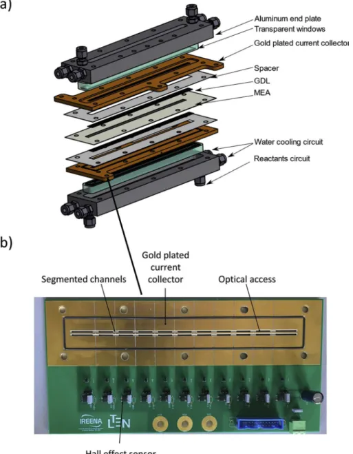
Figure 2. (a) 3D rendering view of the single cell used in the experiments. (b), segmented current collector used to measure the current density distribution. It replaces one of the copper current collector in the single cell.
Journal of Power Sources 440 (2019) 227100 5 jZj ¼ � � � � Rct ~ Zðτc;λÞ � � � � 1 ; (16)
with Rct ¼b=j0. Thus, the modulus is governed by τc, λ, and the cell
electrochemical parameters. In absence of knowledge of b and j0 it is not
possible to predict the modulus of the stoichiometric regime. However, Equation (16) is used at the end the next section to validate the model after measuring the Tafel slope.
2.3. Experimental measurements
Two kinds of experiments are performed in this study to validate both the steady state model using the current density distribution measurements and the periodic state using the EIS response of the fuel cell. To measure the local current density distributions, a segmented flow field was built directly onto a printed circuit board (PCB), see Fig. 2, where the current is measured through eleven segments. Each segment is connected in series to a Hall effect current sensor (Allegro Micro-system, ACS723LLCTR-05AB-T), which converts the current that flows through the segment into voltage. All the 11 voltages are then read by a data acquisition system every second. Each sensor was carefully cali-brated prior to the fuel cell current measurements (see section S1 in supplementary material). According to the datasheet of the sensor and all the experimental uncertainties, it is assumed that the current den-sities are measured with an accuracy of �10%. Such uncertainty was also verified when comparing the current measured by the segmented flow field to the current read by the fuel cell test station (see details in the supplementary materials).
The position, the area and the length of each segment are summar-ised in Table 1. The segmented flow field was gold plated to ensure minimal contact resistance and to prevent copper oxidation when placed inside the cell. Holes were drilled into the flow field to allow an optical access and verify that no liquid water was present in the channel as assumed in the model. The segmented flow field is inserted at the anode side.
The second kind of measurements are the classical EIS. To do so, the fuel cell was connected to a FCT 50 test station (BioLogic®) to measure the cell current, voltage and impedance. The fuel cell impedance was recorded from 10 kHz to 0.1 Hz with 10 points per decade using an AC sine wave signal equal to 10% of the DC current. The FCT 50 test station was also used to control air and hydrogen flow rates, temperatures, humidity and pressure. The protocol used to record EIS data is detailed in supplementary materials.
In all the experiments, a 12 cm2 (200 mm-long by 6 mm-wide) single
cell was used to validate the model. It comprises two parallel channels of 200 mm-long by 1.5 mm-deep. At the cathode side, the flow field was machined directly in the copper current collector to enable an optical access inside the channels via a transparent plexiglass plate inserted on the top of the channels (see Fig. 2(b)). The current collector was gold plated to ensure minimal ohmic resistance (and large Wa). Between the current collectors, a membrane electrode assembly (MEA) was inserted; it is made of a 15 μm-thick Gore PEM with 0.5 mg/cm2 platinum loading in both anode and cathode CL. The very thin membrane and high plat-inum loading were specially chosen to ensure low membrane resistance and efficient electrochemical reaction which match our model as-sumptions (negligible ohmic losses in the membrane and no over-potential gradients in the CL). The MEA was sandwiched between two 10BC GDLs from SGL® compressed at 250 μm using two rigid spacers.
Finally, two aluminum end-plates were used to assemble all the fuel cell components. A water cooling circuit connected to a temperature control system was drilled inside the end plates to keep the fuel cell temperature constant at 70 �C.
Hydrogen flow rate was kept constant throughout all the measure-ments at 300 ml/min, 70 �C and 30% relative humidly to ensure enough
membrane hydration and negligible overpotential losses in the anode. The air flow rate was modulated based on the desired stoichiometry, but for all the experiments air enters fully dry at a fixed temperature of 70 �C
at the cell inlet.
The oxygen stoichiometry and oxygen residence time are computed based on the experimental conditions. The mean air density in the cathode channel is estimated as follows:
ρair¼ Ptot
RTðxH2OMH2OþxO2MO2þxN2MN2Þ; (17)
with xO2¼0:79=0:21 xN2 and xN2 þx02þxH2O ¼1. Although the cell is
fed using dry air, the water produced by the electrochemical reaction makes the air relative humidity close to 100%. Therefore, it is assumed that xH2O ¼PsatðTÞ=Ptot. The relationship (15) is then used to compute
the air flow rate at the cell temperature and pressure, i.e.: _QðT; pÞ ¼ _
QSCPT:ρSCPT=ρair where _QSCPT and ρSCPT are the flow rate and the density
of air in standard condition of pressure and temperature. Then, the ox-ygen stoichiometry is obtained as
λ ¼QðT; pÞc_ ref Icell=ð4FÞ
; (18)
where _QðT; pÞ is the volume flow rate given for the cell operating pres-sure and temperature, Icell is the cell operating current, and cref is the
oxygen concentration at the channel inlet given by the ideal gas law as:
cref¼xinlet O2
ptot
RT; (19)
where xinlet
O2 is the inlet oxygen mole fraction taken to be 0.21 as dry air is
used, and ptot is the total air pressure in the fuel cell.
The model derived in section 2.1 is based on a two-dimensional (2D) geometry which does not take into account the effect of the ribs. Therefore, the velocity defined in Equation (1) is a 2D velocity that would flow without any rib. Experimentally the 2D velocity is given by
u2D c ¼ _ QðT; pÞ lchc ; (20)
where lc is the cell width, e.g. 6 mm. Finally, the oxygen residence time
is based on the u2D c as τc¼ Lc u2D c : (21)
In our flow field geometry, the ratio of the cell active surface to the channel surface is 0.5, thus u2D
c is equal to the half the 3D velocity that
flows inside the fuel cell channels. 3. Results & discussion
3.1. Multiscale evidence of the stoichiometric regime
Before to be able to use the stoichiometric model to characterize the
Table 1
Geometrical characteristics of the segmented current collector.
Segment # 1 2 3 4 5 6 7 8 9 10 11
Length (mm) 19 18 18 18 18 18 18 18 18 18 19
Area (cm2) 1.14 1.08 1.08 1.08 1.08 1.08 1.08 1.08 1.08 1.08 1.14
Dimensionless position 0.95 0.86 0.77 0.68 0.59 0.50 0.41 0.32 0.23 0.14 0.05
Journal of Power Sources 440 (2019) 227100
fuel cell electrochemical kinetics, evidences of the stoichiometric re-gimes have to be observed. This was done at the previously mentioned scales: at the global scale where the EIS signatures at low frequency are measured and at the local scale based on the current density distribution measurements.
3.1.1. At the global scale using low frequency EIS measurements
Like in the authors’ previous works [16], the low frequency EIS signature is used to evidence the stoichiometric regime. In the previous section, it was shown that the low frequency phase in the stoichiometric regime is a function of τc and λ (see Equation (15)), so it can be predicted
easily knowing the fuel cell operating conditions. The low frequency fuel cell phase is measured from the fuel cell impedance as follows: tanφexp¼ Im Zexp � Re Zexp � rHF ; (22)
where Zexp is the measured fuel cell impedance, and rHF is the high
frequency resistance taken as the average of the real part of the fuel cell impedance between 10 Hz and 5 kHz. rHF is subtracted from the fuel cell
impedance to match the assumption of negligible charge transport in the model. The fuel cell phase is measured for a range of oxygen stoichi-ometries and fuel cell currents. Details about the operating conditions used can be found in Table (2).
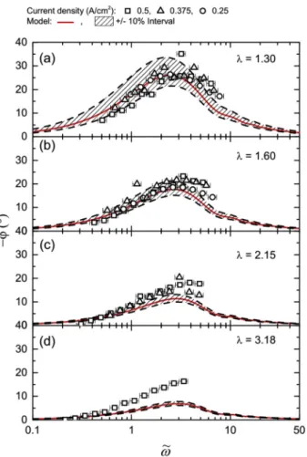
The comparison between Equation (15) and the low frequency phase measurements (Equation (22)) for a range of oxygen stoichiometries and a range of currents is presented in Fig. 3. The model is computed for the stoichiometry at which the cell is operating (see Equation (18)) and an interval at �10% of this oxygen stoichiometry is depicted in dash line. To validate that the cell is operating in stoichiometric regime one can
expect that the measured fuel cell phases fall within this interval. As it can be observed in Fig. 3, this is particularly true at λ ¼ 1.30 and 1.60 for all the currents (0.25, 0.375 and 0.5 A/cm2). However, more deviation is
noticed at λ ¼ 2.15, and the measured phase is out of the interval at λ ¼3.15. Therefore, it can be concluded that the cell is operating in stoichiometric regime for a range of stoichiometric from 1.30 to 2.15 for all the currents tested. This result is in line with the work reported in Ref. [16], and confirms that the assumption made concerning negligible ohmic losses in the membrane and the absence of overpotential gradient in the CL are valid.
Another interesting result concerns the scaling of all the measure-ments regardless the operating current used. This confirms that the low frequency phase depends only on the oxygen stoichiometry when plotted as a function of ~ω. If the same data were plotted versus the
angular frequency, the effect of the operating current would have been shown through a shift of the maximum of the fuel cell phase (see Ref. [16]).
3.1.2. At the local scale using current density distribution measurements
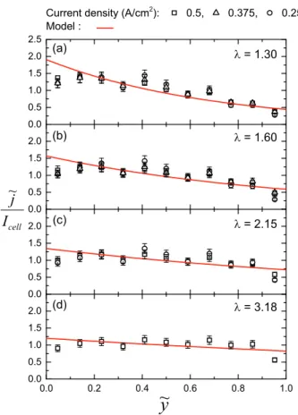
The same kind of evidence of the stoichiometric regime is now sought at the local scale. In the stoichiometric regime the current dis-tribution is given by equation (9). If the measurements of the current in each segment follow the same distribution, then one can conclude that the fuel cell is operating in the stoichiometric regime.
The same operating conditions previously mentioned in Table 2 are used, and the results are presented in Fig. 4. The methodology to compute the error bars on the dimensionless currents is detailed in ap-pendix. Globally, it can be noticed that the measurements agree well with the model regardless the operating currents used and the oxygen stoichiometries. For each stoichiometry, all the data points scale with the model with a very small dispersion with respect to the current level, concluding – once again – that only the stoichiometry governed the current distribution not the value of the current itself justifying the name of stoichiometric regime. Therefore, from the results presented in Fig. 4 and associated to those in Fig. 3, it is concluded that the fuel cell operates in stoichiometric regime for all the operating conditions given in Table 2.
As noticed in Fig. 4(d), surprisingly, the stoichiometric regime may still occur at λ ¼ 3.15 also whereas it was not identified on the low frequency phase (see Fig. 3). This result may be due to some transients’ phenomena which hinder the frequential signature such as oxygen transport delay in the GDL. When λ increases, τc also increases to the
same order of magnitude than the characteristic time of the GDL oxygen transport (see Ref. [16]). Thus, it may be concluded that the measure-ments of the current density distribution would be a more reliable technique to evidence the stoichiometric regime since they are not perturbed by GDL transient phenomena.
The model and the measurements are observed to deviate the most at the cell extremities, i.e. at ~y � 0:05 and 0.95. At the channel inlet, air enters dry and become humidified after few millimetres. The membrane humidity could therefore be lower at the first segment leading to a lower
Fig. 3. Fuel cell low frequency phase measured by EIS for a range of current and oxygen stoichiometry.
Table 2
Summary of the operating conditions used in the stoichiometric regime.
Current density (A/ cm2) Air flow rate (ml/ min) Pressure (bar) ρair (kg/ m3) u(m/s) c λ τc 0.5 123 1.9 2.82 0.31 1.29 0.64 0.25 63 1.87 2.79 0.16 1.32 1.24 0.375 94 1.98 2.904 0.24 1.313 0.86 0.5 153 2.00 2.93 0.39 1.6 0.53 0.25 78 2.02 2.92 0.20 1.63 1.05 0.375 113 1.97 2.894 0.29 1.578 0.72 0.5 204 1.94 2.85 0.52 2.14 0.39 0.25 103 1.90 2.16 0.26 2.16 0.77 0.5 304 2.013 2.93 0.78 3.18 0.27 S. Chevalier et al.
Journal of Power Sources 440 (2019) 227100
7
current production. This effect was observed in the literature on a larger scale [40,45], but here due to the very thin membrane used (15 μm), this non-uniform membrane humidity is only located at the first segment. A second source of uncertainty in the local current density measurement can stem from the uncertainty of the area of the MEA in the segments located at the extremities. During the fuel cell assembly with the segmented current collector, the MEA may have moved a bit toward one of the cell extremities (few millimetres) changing the surface area in contact with the segments at the extremities. This effect was pointed out by Kulkarni et al. [46] using X-rays radiography.
3.2. Characterisation of kinetic parameters in stoichiometric regime 3.2.1. Parameters identification
In the previous section, it was shown that the fuel cell is operating in the stoichiometric regime, validating the use of equations (1) and (2) to model the fuel cell behavior. Using these equations, one can show that
c0
cðyÞ =cref ¼e λ*y~, and j0 ¼iceη=b. Thus, by integrating equation (1) it
leads to: Icell¼ Z1 0 jð~yÞd~y ¼ iceη=b Z1 0 e λ*~yd~y ¼iceη=b λλ* : (23)
Equation (23), is then rewritten in linear form using the decimal logarithm to obtain:
η¼2:3b � logðIcellλλ*Þ 2:3b � logðicÞ: (24)
Equation (24) can be viewed as the Tafel equation but for a 2D cell where the current density Icell is corrected by the effect of the
stoichi-ometry in the channel, i.e. λλ*. Thus, by measuring the cell overpotential
and current density, it is possible to accurately fit the Tafel slope and the exchange current density to characterize the cell electrochemical kinetics.
In Fig. 5, the overpotential measurement versus the corrected current density is shown for all the measurements summarised in Table 2. The methodology to compute the uncertainty of the current density is explained in appendix. The overpotential is computed as
η¼1:23 Ecell rHF�Icell; (25)
where Ecell, rHF and Icell are the cell voltage, ohmic resistance and current
density measured. These values are summarised in Table 3. Using equation (24) and a linear regression, the Tafel slope and the exchange current are obtained (see Table 3 for the values).
In their review, Eslamibidgoli et al. [3] recalled that three regimes of electrochemical kinetics are theoretically expected. From medium to high overpotentials, these regimes are characterised by a value of Tafel slope that varies from 80 mV to 120 mV [3]. Our results presented in Fig. 5 show a similar trend where the slope varies between the data points measured at medium and high overpotential with a Tafel slope equal to 143 � 21 mV and 229 � 52 mV, respectively. We found that the value of the Tafel slope is larger than what is theoretically predicted, but the ratio between them is correct (2/3). The larger than expected Tafel slopes measured in his study are in-situ values in sense that some other physical phenomena may have impacted it: heterogeneities in the fuel cell assembly, effect of the channel/rib, catalyst degradations/aging. However, this Tafel slope can be considered as the correct values in the framework of the stoichiometric regime and become an accurate crite-rion to assess the kinetic performances of different fuel cell assemblies for example.
A similar conclusion can be drawn concerning the values of the ex-change currents. We found two regimes at medium and high over-potential where the values of ic vary significatively. Although it is
difficult to link these in situ values to fuel cell characteristics (platinum loading, ECSA, catalyst layer composition …), they can be used in the similar way as the Tafel slope: using ic to characterize the fuel cell
ki-netics in the framework of the stoichiometric regime and compare them to study different catalyst layer or aging impact for example.
3.2.2. Model validation
Going further to validate the consistency of the measured value of b and ic with the stoichiometric regime, we check the assumption made in
section 2 where αc¼ic=j0eηðtÞ=b�1. In the stoichiometric regime, we can write that αc¼iceηðbtÞ=ðIcellλλ*Þ:These values are computed in Table 3. As it can be observed, αc is found to be very close to 1 validating the
assumption made earlier and meaning that the value b and ic are Fig. 4. Non-dimensional local current density distributions for a range of
current and oxygen stoichiometry.
Fig. 5. Linear fit of the Tafel slope and exchange current density in the stoi-chiometric regime.
Journal of Power Sources 440 (2019) 227100
consistent with the assumptions made to derive the stoichiometric model.
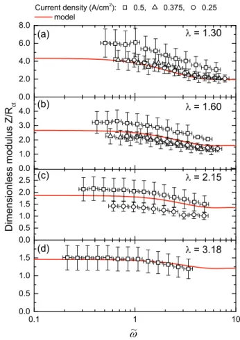
The second validation is based on the fuel cell impedance modulus. Only the phase was used previously to verify that the fuel cell is oper-ating in stoichiometric regime. To compute the dimensionless fuel cell impedance, ��Zexp��, the charge transfer resistance is needed as it is shown in Equation (16). The charge transfer resistance is given by Rct¼b= ðj0Þ with j0¼Icellλλ* according to Equation (23). The uncertainty associated
to the dimensionless modulus is given in appendix. These data are pre-sented in Fig. 6 and compared to the modulus of the impedance in stoichiometric regime given by Equation (14) as j~Zj ¼ j1=~Zj 1.
The experimental modulus measured in stoichiometric regime scales quite well with the model (red lines in Fig. 6) for all the oxygen stoi-chiometries. Although some deviations can be observed (at λ ¼ 2.15 and 3 A for example), the general trend is well reproduced. This result shows that the fuel cell can be fully characterized where all the parameters of the stoichiometric regime can be measured (membrane resistance, electrochemical kinetics, oxygen transport in the channel) and used to predict both the steady state of the cell (current and current density) and periodic state (fuel cell impedance).
4. Conclusions
The aim of this paper was to evidence the stoichiometric regime in an operating fuel cell both at the global and local scale using EIS mea-surements and current density distribution meamea-surements with a segmented flow field. This was successfully done for a range of stoi-chiometry from 1.30 to 3.18 and a range of current from 3 A to 6 A (0.25–0.5 A/cm2). At the local scale it may have been easier to evidence
the stoichiometric regime, particularly at λ ¼ 3.18 where the low fre-quency phase can be altered by the oxygen transport in the GDL (see Ref. [16]). However, the use of segmented cell is not mandatory to obtain a signature of the stoichiometric regime since it is well observed through the low frequency phase for most of the measurements pre-sented in this paper.
Operating a fuel cell in this particular regime is a great advantage from the modelling point of view as only two equations govern the main physical mechanisms. Therefore, few parameters are needed to predict the fuel cell behavior. Moreover, in the case they are not known, such as the kinetics parameters (Tafel slope and exchange current), a method-ology is presented to measure them accurately. Thus, within the framework of this stoichiometric regime, PEM fuel cells can be better controlled, their performances better predicted, and their physical properties better characterized.
Another application of these works concerns the hydrogen/oxygen fuel cells where mass transport in the GDL are not limiting. Thus, these fuel cells operating conditions fall within the assumption needed to derive the stoichiometric regime, and our work can be transpose to this
technology to characterize the kinetic parameters or to control hydrogen/oxygen fuel cell performances.
Acknowledgements
The research leading to these results received funding from the People Programme (Marie Curie Actions) of the European Union’s Seventh Framework Programme (FP7/2007–2013) under REA grant agreement n� PCOFUND-GA-2013-609102, through the PRESTIGE
programme coordinated by Campus France. The authors would like to gratefully acknowledge Mr Christophe Le Bozec for his help in designing and building the experimental setup.
Table 3
Summary of the fuel cell characterisation in stoichiometric regime for a range of current and oxygen stoichiometry.
Current (A) Icell (A/cm2) λ rHF (mΩ) E (V) η (V) b (mV) s(mA/cm2) αc
6 0.500 1.29 13 0.53 0.62 229 � 52 65 � 18 1,01 3 0.250 1.32 16 0.69 0.49 143 � 21 21 � 4 0,96 4.5 0.375 1.31 15 0.64 0.52 229 � 52 65 � 18 0,89 6 0.500 1.60 13 0.60 0.55 229 � 52 65 � 18 0,91 3 0.250 1.63 16 0.71 0.47 143 � 21 21 � 4 1,01 4.5 0.375 1.58 15 0.68 0.48 229 � 52 65 � 18 0,89 6 0.500 2.14 13 0.60 0.55 229 � 52 65 � 18 1,06 3 0.250 2.16 14 0.74 0.45 143 � 21 21 � 4 1,01 6 0.500 3.18 13 0.65 0.51 229 � 52 65 � 18 1,00
Fig. 6. Impedance modulus versus dimensionless frequency for a range of air stoichiometry and cell current.
Journal of Power Sources 440 (2019) 227100
9
Appendix. Uncertainty calculations
Dimensionless current
We consider that the N current densities measured by the segmented current collector are known within �10% of the measured value. So, the uncertainty on the mean value is:
umean¼ 0:1 N ffiffiffiffiffiffiffiffiffiffiffi XN n¼1 j2 n v u u t ; (A.1)
This is the root sum of squares of the measured current density.
Thus, one can deduce that the uncertainty of the dimensionless current is:
uIadim¼0:1Iadim
ffiffiffiffiffiffiffiffiffiffiffiffiffiffiffiffiffiffiffiffiffiffiffi 1 þ PN n¼1j2n N2I2 mean s ; (A.2)
Flow rate, velocity and stoichiometry
In this study, the air flow rate, velocity and stoichiometry are considered to be known at �10%. This uncertainty stems from the mass flow controller, the cell temperature controller and the back pressure controller. For sake of simplicity, all these uncertainties are embedded in a single one where the velocity is assumed to known at �10% of uc.
Tafel slope
Calculation of the uncertainty on the Tafel slope and the exchange current density obtained from the linear fit. For the Tafel slope, it is trivial: ub¼
ua1=2:3 where ua1 is the uncertainty computed by the linear fit including the weight of each data (error bar on x-axis). Concerning the exchange
current, it is given by the following formula: ic¼10 a2=a1 where a1 and a2 are the slope and the intercept, respectively. Thus, the uncertainty on ic is
given by: u2 ic¼ � ua1 ∂ic ∂a1 �2 þ � ua2 ∂ic ∂a2 �2 ; (A.3) which lead to uic¼ic ffiffiffiffiffiffiffiffiffiffiffiffiffiffiffiffiffiffiffiffiffiffiffiffi u2 a2 a2 2 þu 2 a1 a2 1 a2 2 a2 1 s : (A.4) Modulus
The uncertainty of the modulus depends of the uncertainty of the charge transfer resistance computed as:
u2 Rct¼ � ub λλ*Icell �2 þu2 λ b2 I2 cell � ð1 λÞλ*þ1 ð1 λÞλ*2λ2 �2 ; (A.5) which lead to u2 Rct R2 ct ¼�ub b �2 þu 2 λ λ2 � ð1 λÞλ*þ1 ð1 λÞλ* �2 : (A.6)
where uλ¼0:1 � λ and ub is given in Table 3. Finally, one can obtain
uRct¼Rct ffiffiffiffiffiffiffiffiffiffiffiffiffiffiffiffiffiffiffiffiffiffiffiffiffiffiffiffiffiffiffiffiffiffiffiffiffiffiffiffiffiffiffiffiffiffiffiffiffiffiffiffiffiffiffiffiffiffiffiffiffi �ub b �2 þ0:12 � ð1 λÞλ*þ1 ð1 λÞλ* �2 s ; (A.7)
and, the uncertainty on the dimensionless modulus is given by
uj~Zj¼ j~ZjuRct Rct
: (A.8)
Appendix A. Supplementary data
Supplementary data to this article can be found online at https://doi.org/10.1016/j.jpowsour.2019.227100.
Journal of Power Sources 440 (2019) 227100
References
[1] N. Konno, S. Mizuno, H. Nakaji, Y. Ishikawa, Development of compact and high- performance fuel cell stack, SAE Int. J. Altern. Powertrains. 4 (1) (2015) 123–129,
https://doi.org/10.4271/2015-01-1175, 01–1175.
[2] T. Yoshida, K. Kojima, Toyota MIRAI fuel cell vehicle and progress toward a future hydrogen society, Interface Mag 24 (2015) 45–49.
[3] M.J. Eslamibidgoli, J. Huang, T. Kadyk, A. Malek, M. Eikerling, How theory and simulation can drive fuel cell electrocatalysis, Nano Energy 29 (2016) 334–361. [4] A.Z. Weber, R.L. Borup, R.M. Darling, P.K. Das, T.J. Dursch, W. Gu, et al., A critical
review of modeling transport phenomena in polymer-electrolyte fuel cells, J. Electrochem. Soc. 161 (2014) F1254–F1299.
[5] A.Z. Weber, J. Newman, Modeling transport in polymer-electrolyte fuel cells, Chem. Rev. 104 (2004) 4679–4726.
[6] A.A. Kulikovsky, The effect of stoichiometric ratio λ on the performance of a polymer electrolyte fuel cell, Electrochim. Acta 49 (2004) 617–625.
[7] J.T. Gostick, Versatile and efficient pore network extraction method using marker- based watershed segmentation, Phys. Rev. E. 96 (2017), 023307.
[8] L. Cindrella, A.M. Kannan, J.F. Lin, K. Saminathan, Y. Ho, C.W. Lin, J. Wertz, Gas diffusion layer for proton exchange membrane fuel cells—a review, J. Power Sources 194 (2009) 146–160.
[9] G. Zhang, K. Jiao, Multi-phase models for water and thermal management of proton exchange membrane fuel cell: a review, J. Power Sources 391 (2018) 120–133.
[10] B.P. Setzler, T.F. Fuller, A physics-based impedance model of proton exchange membrane fuel cells exhibiting low-frequency inductive loops, J. Electrochem. Soc. 162 (2015) F519–F530.
[11] Y. Wang, S. Basu, C.-Y. Wang, Modeling two-phase flow in PEM fuel cell channels, J. Power Sources 179 (2008) 603–617.
[12] T.E. Springer, T.A. Zawodzinski, S. Gottesfeld, Polymer electrolyte fuel cell model, J. Electrochem. Soc. 138 (1991) 2334.
[13] A.A. Kulikovsky, A simple equation for in situ measurement of the catalyst layer oxygen diffusivity in PEM fuel cell, J. Electroanal. Chem. 720–721 (2014) 47–51. [14] A.A. Kulikovsky, The regimes of catalyst layer operation in a fuel cell, Electrochim.
Acta 55 (2010) 6391–6401.
[15] S. Chevalier, C. Josset, B. Auvity, Analytical solutions and dimensional analysis of pseudo 2D current density distribution model in PEM fuel cells, Renew. Energy 125 (2018) 738–746.
[16] S. Chevalier, C. Josset, B. Auvity, Analytical solution for the low frequency polymer electrolyte membrane fuel cell impedance, J. Power Sources 407 (2018) 123–131. [17] J. Xuan, H. Wang, D.Y.C. Leung, M.K.H. Leung, H. Xu, L. Zhang, Y. Shen,
Theoretical Graetz–Damk€ohler modeling of an air-breathing microfluidic fuel cell, J. Power Sources 231 (2013) 1–5.
[18] G. Maranzana, J. Mainka, O. Lottin, J. Dillet, A. Lamibrac, A. Thomas, S. Didierjean, A proton exchange membrane fuel cell impedance model taking into account convection along the air channel: on the bias between the low frequency limit of the impedance and the slope of the polarization curve, Electrochim. Acta 83 (2012) 13–27.
[19] K.T. Jeng, C.P. Kuo, S.F. Lee, Modeling the catalyst layer of a PEM fuel cell cathode using a dimensionless approach, J. Power Sources 128 (2004) 145–151. [20] O. Shamardina, M.S. Kondratenko, A.V. Chertovich, A. Kulikovsky, A simple
transient model for a high temperature PEM fuel cell impedance, Int. J. Hydrogen Energy 39 (2014) 2224–2235.
[21] J.-C. Olivier, G. Wasselynck, S. Chevalier, B. Auvity, C. Josset, D. Trichet, G. Squadrito, N. Bernard, Multiphysics modeling and optimization of the driving strategy of a light duty fuel cell vehicle, Int. J. Hydrogen Energy 42 (2017) 26943–26955.
[22] N. Fouquet, C. Doulet, C. Nouillant, G. Dauphin-Tanguy, B. Ould-Bouamama, Model based PEM fuel cell state-of-health monitoring via ac impedance measurements, J. Power Sources 159 (2006) 905–913.
[23] I. Manke, C. Hartnig, M. Grünerbel, W. Lehnert, N. Kardjilov, A. Haibel, A. Hilger, J. Banhart, H. Riesemeier, Investigation of water evolution and transport in fuel cells with high resolution synchrotron x-ray radiography, Appl. Phys. Lett. 90 (2007) 174105.
[24] J. Lee, S. Chevalier, R. Banerjee, P. Antonacci, N. Ge, R. Yip, T. Kotaka, Y. Tabuchi, A. Bazylak, Investigating the effects of gas diffusion layer substrate thickness on
polymer electrolyte membrane fuel cell performance via synchrotron X-ray radiography, Electrochim. Acta 236 (2017) 161–170.
[25] D. Hayashi, A. Ida, S. Magome, T. Suzuki, S. Yamaguchi, R. Hori, Synchrotron X- Ray Visualization and Simulation for Operating Fuel Cell Diffusion Layers, 2017. [26] Q. Meyer, Y. Zeng, C. Zhao, In situ and operando characterization of proton
exchange membrane fuel cells, Adv. Mater. (2019) 1901900.
[27] G. Hinds, In situ diagnostics for polymer electrolyte membrane fuel cells, Curr. Opin. Electrochem. 5 (2017) 11–19.
[28] J.E.B. Randles, Kinetics of rapid electrode reactions, Discuss. Faraday Soc. 1 (1947) 11–19.
[29] P. Antonacci, S. Chevalier, J. Lee, N. Ge, J. Hinebaugh, R. Yip, Y. Tabuchi, T. Kotaka, A. Bazylak, Balancing mass transport resistance and membrane resistance when tailoring MPL thickness for PEM fuel cells, Electrochim. Acta 188 (2016) 888–897.
[30] T.E. Springer, T.A. Zawodzinski, M.S. Wilson, S. Golfesfeld, Characterization of polymer electrolyte fuel cells using AC impedance spectroscopy, J. Electrochem. Soc. 143 (1996) 587–599.
[31] D. Kramer, I.A. Schneider, A. Wokaun, G.G. Scherer, Oscillations in the gas channels - the forgotten player in impedance spectroscopy in polymer electrolyte fuel cells B. Modeling the wave, in: E.C.S. Trans (Ed.), ECS, 2006, pp. 1249–1258. [32] S.M. Rezaei Niya, M. Hoorfar, Study of proton exchange membrane fuel cells using electrochemical impedance spectroscopy technique – a review, J. Power Sources 240 (2013) 281–293.
[33] L.C. P�erez, L. Brand~ao, J.M. Sousa, A. Mendes, Segmented polymer electrolyte membrane fuel cells—a review, Renew. Sustain. Energy Rev. 15 (2011) 169–185. [34] I.A. Schneider, D. Kramer, A. Wokaun, G.G. Scherer, Oscillations in gas channels:
II. Unraveling the characteristics of the low frequency loop in air-fed PEFC impedance spectra, J. Electrochem. Soc. 154 (2007) B770–B782.
[35] Q. Meyer, K. Ronaszegi, J.B. Robinson, M. Noorkami, O. Curnick, S. Ashton, A. Danelyan, T. Reisch, P. Adcock, R. Kraume, P.R. Shearing, D.J.L. Brett, Combined current and temperature mapping in an air-cooled, open-cathode polymer electrolyte fuel cell under steady-state and dynamic conditions, J. Power Sources 297 (2015) 315–322.
[36] T. Reshetenko, A. Kulikovsky, Comparison of two physical models for fitting PEM fuel cell impedance spectra measured at a low air flow stoichiometry, J. Electrochem. Soc. 163 (2016) F238–F246.
[37] N. Zamel, A. Bhattarai, D. Gerteisen, Measurement of spatially resolved impedance spectroscopy with local perturbation, Fuel Cells 13 (2013) 910–916.
[38] G. Maranzana, O. Lottin, T. Colinart, S. Chupin, S. Didierjean, A multi- instrumented polymer exchange membrane fuel cell: observation of the in-plane non-homogeneities, J. Power Sources 180 (2008) 748–754.
[39] A. Kulikovsky, Analytical impedance of oxygen transport in a PEM fuel cell channel, J. Electrochem. Soc. 166 (2019) F306–F311.
[40] I.A. Schneider, S.A. Freunberger, D. Kramer, A. Wokaun, G.G. Scherer, Oscillations in gas channels. Part I. The forgotten player in impedance spectroscopy in PEFCs, J. Electrochem. Soc. 154 (2007) B383–B388.
[41] I. Pivac, F. Barbir, Inductive phenomena at low frequencies in impedance spectra of proton exchange membrane fuel cells – a review, J. Power Sources 326 (2016) 112–119.
[42] I.J. Halvorsen, I. Pivac, D. Bezmalinovi�c, F. Barbir, F. Zenith, Electrochemical low- frequency impedance spectroscopy algorithm for diagnostics of PEM fuel cell degradation, Int. J. Hydrogen Energy (2019).
[43] S. Chevalier, N. Ge, J. Lee, M.G. George, H. Liu, P. Shrestha, D. Muirhead, N. Lavielle, B.D. Hatton, A. Bazylak, Novel electrospun gas diffusion layers for polymer electrolyte membrane fuel cells: Part II. In operando synchrotron imaging for microscale liquid water transport characterization, J. Power Sources 352 (2017) 281–290.
[44] T. Reshetenko, A. Kulikovsky, On the distribution of local current density along a PEM fuel cell cathode channel, Electrochem. Commun. 101 (2019) 35–38. [45] A.A. Kulikovsky, Semi-analytical 1Dþ1D model of a polymer electrolyte fuel cell,
Electrochem. Commun. 6 (2004) 969–977.
[46] N. Kulkarni, Q. Meyer, J. Hack, R. Jervis, F. Iacoviello, K. Ronaszegi, P. Adcock, P. R. Shearing, D.J.L. Brett, Examining the effect of the secondary flow-field on polymer electrolyte fuel cells using X-ray computed radiography and computational modelling, Int. J. Hydrogen Energy 44 (2019) 1139–1150.