CIRPÉE
Centre interuniversitaire sur le risque, les politiques économiques et l’emploi
Cahier de recherche/Working Paper 05-22
When is Economic Growth Pro-Poor? Evidence from Tunisia
Sami Bibi
Juillet/July 2005
_______________________
Bibi: Centre Interuniversitaire sur le Risque, les Politiques Économiques et l’Emploi (CIRPÉE) and Faculté des Sciences Économiques et de Gestion de Tunis (FSEGT), Campus Universitaire, BP 248, El Manar, C.P. 2092, Tunis, Tunisia. Fax: 216-71-93-06-15
I am grateful to Jean-Yves Duclos, Rim Limam, Dorra Touzri and Hedia Chtioui for their helpful comments. The usual disclaimer applies.
Abstract:
Many empirical studies have shown that economic growth generally leads to a drop in poverty. These studies have also pointed out that a given growth rate is compatible with a large range of outcomes in terms of poverty reduction. This means that growth is more pro-poor in certain cases than in others. Using complete and partial poverty orderings, this paper suggests a measure which captures the extent to which economic growth is pro-poor. This measure decomposes poverty changes into two components : the relative variation in the average income of the poor and the relative variation in the overall inequality within the poor. Evidence from Tunisia shows that economic growth was to a large extent pro-poor during the last two decades.
Keywords: Poverty measurement, Robustness analysis, Economic growth, Tunisia JEL Classification: D31, D63, I32, O40
1
Introduction
Absolute poverty is bound to decrease whenever economic growth affects pos-itively the less well-off. Thus, under such a situation, growth can plausibly be deemed pro-poor. Yet if the income of the richest grows faster than the income of the poorest, growth will be accompanied by a rise in overall inequality, which will increase relative poverty. Thus, while growth can often be considered pro-poor, it can certainly be less pro-poor than a growth pattern which increases more the income of the poorest.
The extent to which growth is pro-poor has become a hotly debated subject.1
Answering this question requires solving the identification and the aggregation issues. It is well-known, however, that the measurement of poverty is to a large extent arbitrary. Measuring the extent to which growth is pro-poor requires choos-ing selectively among a very large number of available poverty indices. It also involves estimating some poverty lines through procedures that are typically sen-sitive to many crucial ethical and statistical assumptions. Hence, it is not surpris-ing that measursurpris-ing pro-poor growth on the basis of such poverty assessment may also be considered arbitrary. Our objective in this paper is to curb such degrees of arbitrariness by characterizing the growth pattern for a large range of poverty lines and for classes of poverty indices of some ethical order.
This goal is achieved in two steps. First, we use complete poverty orderings to develop a measure that captures the extent to which economic growth is pro-poor. Second, and building on the important contributions of Ravallion and Chen (2003) and Son (2004), we develop the requirements of pro-poor growth using partial poverty orderings. While these papers focus on first- and second-order pro-poor growth, respectively, this one considers, however, the growth patterns for various orders of ethical principles. Applying the methodology to Tunisian data, we find that economic growth was to a large extent pro-poor during the last two decades.
The rest of this paper is structured as follows. Section 2 summarizes the theo-retical framework related to the link between economic growth and poverty reduc-tion and suggests a new index that captures the extent to which growth is pro-poor given a pre-selected poverty measure. Section 3 describes how to check for the ethical robustness of pro-poor growth. Section 4 computes the extent to which growth was pro-poor during the last two decades in Tunisia. Section 5 offers
1See, among many others, Kakwani and Pernia (2000), Ravallion and Chen (2003), Duclos
some concluding remarks.
2
Growth contribution to poverty reduction
To assess whether the observed change in the distribution of income is pro-poor, it is conventional to decompose the change in poverty into a change related to an
uniform growth of income and a change in relative incomes.2 However, as argued
by Ravallion and Chen (2003), it is possible that while the distributional changes are pro-poor, there is no absolute gain to the poor.
A more direct approach is to look at growth rates among the poor. For this, let
y(p) be the quantile function of living standards (incomes, for short) for p ∈ [0, 1].
For a continuous and strictly increasing distribution, yt(p) is then the individual’s
income whose percentile is p at time t. Further, let g0t(x) be the growth rate in the
variable x between t and t − 1.
To describe how poverty is affected by economic growth, we must also address the measurement of poverty. We start with the popular Foster-Greer-Thorbecke (1984) (FGT) class of poverty indices, although an important aim of this paper is to show how the use of these peculiar indices is also useful for predicting how many other indices will react to the distribution of growth rates. Let z be a real poverty line. The FGT class is then defined as
Pt α(p) = Z p 0 µ z − yt(ρ) z ¶α dρ, (1)
As it is well known, P0(.) = p is the poverty headcount (the ”incidence” of
poverty), P1(.) is the normalized average poverty gap measure (the ”intensity”
of poverty), and P2(.) is often described as an index of the ”severity” of poverty –
it weights poverty gaps by poverty gaps.
We begin by investigating the ideal distribution of economic growth, that is the distribution leading to the least poverty, as defined by an index of the FGT class. The ideal distribution could be of different types. For instance, if α = 0, growth is deemed pro-poor when it brings the richest of the poor out of poverty. Formally, and considering a marginal analysis, pro-poor growth requires that those at the margin of poverty present a positive growth rate of income
gt
0(z(p)) ≥ 0 (2)
Therefore, the headcount ratio only records those growth rates which bring peo-ple out of poverty, that is, only poverty-eliminating growth rates matter and not poverty-alleviating growth rates. As a consequence, the effectiveness of growth cannot be accurately captured when a large number of the poor benefit from eco-nomic growth without escaping poverty.
If the poverty measure is in line with the Sen’s (1976) monotonicity axiom,3
the normalized average poverty gap becomes an appealing poverty index. It is well known that this index falls when the mean income of the population of the poor rises: gt 1(p) = Rp 0 yt(ρ)dρ Rp 0 yt−1(ρ)dρ − 1 ≥ 0 (3)
The pro-poor growth rate given by (3) does not, however, distinguish between growth that enhances the income of the poorest from growth that helps the not-so-poor. Thus, a better pattern of growth satisfies Sen’s (1976) core axioms for poverty measurement, namely the focus axiom, the monotonicity axiom and the
transfer axiom.4
Hence, in the manner of Atkinson (1970) for the measurement of social
wel-fare and inequality, let Γtα(p) be the ”equally-distributed equivalent (EDE) income
of the poor”, viz, that income which, if assigned equally to every one within the poorest pth quantile of the population, would produce the same poverty measure
as that generated by the actual distribution of income. Using (1), Γtα(p) is given
implicitly as Γtα(p) = z à 1 − µ Pt α(p) p ¶1 α ! for α ≥ 1. (4)
By (4), pro-poor growth requires that
gt α(p) = Γt α(p) Γt−1 α (p) − 1 ≥ 0 for α ≥ 1. (5)
Since the growth rates of the non-poor do not matter when measuring gαt(p),
the measure of pro-poor growth given by (5) is in line with the focus axiom for any value of α. The monotonicity axiom is observed when α ≥ 1 and the transfer axiom requires that α > 1.
3According to this axiom, an increase in a poor’s income should decrease the poverty level.
4The focus axiom requires that poverty measures be independent of the income distribution of
the non-poor whereas the transfer axiom asserts that a progressive transfer from a not-so-poor to a poor should decrease the poverty level.
It is of interest to decompose the total impact of economic growth on poverty into the impact of growth when the distribution of income does not change and
the effect of the inequality changes when total income does not change.5 As for
α > 1, the more unequal the distribution of incomes is, the more important the
difference between Γt1(p) and Γtα(p) is;6a natural measure of the equality index is
then given by:
Et α(p) = Γt α(p) Γt 1(p) for α ≥ 1. (6)
Using (6), pro-poor growth can alternatively be expressed as
gαt(p) = g1t(p) + g0t(Eα(p)) for α ≥ 1 (7)
where g1t(p) is the pure growth effect and gt0(Eα(z)) is the equality effect.7 Hence,
and while in Kakwani and Pernia’s (2000) model the pure growth effect is deemed always positive, our model allows for poverty to increase or decrease with growth depending on whether or not, in average, economic growth enhances the poor in-come. The second effect is positive (negative) if those at the bottom of the distri-bution benefit more (less) from economic growth than the not-so-poor. Whenever these two components are positive, economic growth can be deemed really pro-poor. This means that the degree of pro-poor growth can be captured by this index of pro-poor growth ψt α(p) = gt α(p) gt 1(p) for α ≥ 0. (8)
When only poverty-eliminating growth matters, growth is deemed highly
pro-not-so-poor if ψt0(p) > 1, an example of r-type pro-poor growth in Bourguignon
and Fields’s (1997) terminology. Nevertheless, if mainly poverty-alleviating growth matters, growth is deemed pro-poor when it curbs inequality. Indeed, and using equation (7), it is possible to rewrite (8) as follows:
ψt α(p) = 1 + gt 0(Eα(p)) gt 1(p) for α ≥ 1. (9)
5See, for instance, Kakwani and Pernia (2000).
6For a scrutinized description on this, see Bibi and Duclos (2005).
7Using a general formulation of a poverty evaluation function, Kraay (2004) identifies three
sources of pro-poor growth: a high growth rate in the mean income, a high sensitivity of the poverty index to the growth rate in the mean income, and the growth in relative incomes. The first term in equation (7) summarizes the first two sources of Kraay’s (2004) sources of pro-poor growth while the second term of (7) captures the growth in relative incomes. Indeed, if the income of the poorest grows faster than the income of the less-so-poor, then distribution sensitive poverty indices will fall faster.
The interpretation of (9) depends on the sign of ψαt(z) and on whether ψtα(z) is greater, smaller or equal to 1.
• If ψt
α(p) < 0, the growth rates are so much regressively distributed –
neg-ative for the poorest and positive for the less-so-poor – that they offset the
rise in the mean income of the poor and lead to a negative gαt(p).
• If ψt
α(p) ranges between 0 and 1, this means that although economic growth
is well spread among the poor, the less-so-poor benefit more from it which
rises inequality within the poor (g0t(Eα(p)) < 0). However, this rise is not
enough to offset the positive impact of economic growth on the cumulative poor income. Such a situation can therefore receive the label of a regressive pro-poor growth.
• If ψt
α(p) = 1, we are in presence of a distribution-neutral pro-poor growth.
By (9), this case occurs when gt0(Eα(p)) = 0, meaning that absolute poverty
decreases only as a result of the equally distributed growth rates within the poor.
• If ψt
α(p) > 1, the distributional pattern of economic growth is really
pro-poor. This happens when g0t(Eα(p)) > 0, which indicates that the poorest
benefit more than the not-so-poor from economic growth. This growth pat-tern can be labelled as a progressive pro-poor growth.
Therefore, one condition for growth to be really pro-poor is that ψαt(p) be
greater than 1. Relying on Kakwani and Pernia (2000), this is too strong a condi-tion. Based on their empirical result, growth is deemed to be:
• pro-rich when gt
1(p) < 0 and the growth in the mean income is positive.
This is a case of what Bhagwati (1988) calls immiserizing growth;
• not pro-poor when gt
1(p) = 0, regardless of the value of ψ0t(p).
• regressively pro-poor when gt
1(p) > 0 and ψαt(p) < 0;
• r-type or weakly pro-poor when gt
1(p) > 0, ψαt(p) < 0.33 for α ≥ 2, and/or
ψt
0(p) > 1.33;
• moderately pro-poor if ψt
α(p) ranges between 0.33 and 0.66 for α ≥ 2
• highly enough pro-poor if 0.66 < ψt
α(p) ≤ 1 for α ≥ 2, regardless of the
value of ψ0t(p);
• and really or progressively pro-poor when ψt
α(p) > 1, for α ≥ 2, regardless
of the value of ψt0(p).
3
Robustness analysis
The above analysis clearly depends on the choice of a poverty index and a poverty line. Since both of these choices are typically somewhat arbitrary, so will be the pattern of economic growth characterized using them. We also saw that seeking pro-poor growth on the basis of reducing one poverty index can lead to policies that penalize the poorest of the poor, and can thus raise important ethical issues.
Drawing on and developing results from the theory of stochastic dominance, it is fortunately possible to curb such degrees of arbitrariness by looking at the inter-temporal comparisons of poverty over p and for a class of ”acceptable” poverty indices. The acceptability of poverty indices will depend on whether they meet normative criteria of some ethical order. Each order of normative criteria defines a class of poverty measures. As the ethical order increases, the criteria put in-creasingly strong constraints on the way poverty indices should rank distributions of living standards. Thus, lower degree dominance usually entails higher degree dominance, but the converse does not necessary hold.
To illustrate how to do this, consider the following general utilitarian
formu-lation of a poverty evaluation function:8
Pt(p) = Z Ω Z 1 0 π(yt(p), ωt; z)f (ωt)dωtdp, (10)
where the π(yt(p), ωt; z) are the individual contributions to poverty9. A class
Πt
s(p∗) of poverty evaluation functions (of ethical order s) can then be defined by
putting restrictions on the properties of π(yt(p), ωt; z) and by imposing that p ≤
p∗. A first natural normative property is that π(yt(p), ωt; z) be weakly decreasing
in p, whatever the level of p and whatever the value of ωt. Because the ethical
8For expositional simplicity, we thus focus on additive poverty indices. See inter alia Foster
and Shorrocks (1988) for how non-additive evaluation functions could also be included in the analysis.
9A poverty evaluation function can be thought of as the negative of a social evaluation function
condition imposed for membership in that class is very weak – and is almost
universally accepted10– we can consider that class to be of ethical order 1, and it
can therefore be denoted as Πt1(p∗).
More formally, assume that π(yt(p), ωt; z) is differentiable11 with respect to p
for all p < p∗, and denote by π(s)(yt(p), ωt; z) the s-order derivative of π(yt(p), ωt; z)
with respect to p. Πt1(p∗) can then be defined as:
Πt 1(p∗) = Pt(p) ¯ ¯ ¯ ¯ ¯ ¯ ¯ ¯ p ∈ [0, p∗],
π(yt(ρ), ωt; z) = π(yt(p), ωt; z) for ρ > p,
π(yt(ρ), ωt; z) = π(yt(ρ); z) for ρ ≤ p.
π(1)(yt(ρ); z) ≤ 0. (11)
The first line on the right of (11) defines the population segment used to describe the pattern of growth. The second line on the right of (11) assumes that the poverty measures fulfill the well-known ”poverty focus axiom” – which states that changes in the living standards of the non-poor should not affect the poverty measure. The
third line requires that the social contributions π(yt(p), ωt; z) in (11) should not
depend on the taste parameters ωt, viz, so that the social judgement is anonymous
in the ωt; and (10) can be rewritten asR01π(yt(p); z)dp. The last line assumes that
the Πt1(z∗) indices are weakly decreasing with income.
Bibi and Duclos (2003) show that if poverty, as computed using any poverty
indices within Π1(p), falls, then there is a Pen-improvement of poverty.12
Equiv-alently, growth can be labelled Pen-pro-poor if it raises income at any quantile
below p∗.13 Thus, a necessary and sufficient condition for growth to be
Pen-pro-poor and for first-order poverty-improving – that is, to weakly decrease poverty
for all Pt(p) ∈ Πt1(p∗) – is that
gt
0(p) ≥ 0 for all p ∈ [0, p∗] (12)
Testing solely the FOD conditions could not, however, be really informative
about the distributional pattern of economic growth.14 For instance, if gt
0(p)
ex-10With the exception of relative poverty as an increase in a poor’s living standard can increase
the relative poverty line and possibly the poverty index.
11This differentiability assumption is made for expositional simplicity and could be relaxed.
12See Pen (1971).
13Whenever p∗= 1, there is also a Pen-improvement of welfare.
14To test whether the movement from an initial to a final distribution is pro-poor using FOD
conditions, Duclos and Wodon (2004) (see in particular their Theorem 9) check whether the head-count index in the initial distribution is –regardless of the poverty line chosen– larger than the headcount index in the final distribution when the final distribution is normalized by a standard (1 + g). Note that g can be equal, for instance, to the growth rate in the mean income.
hibits a downward (an upward) sloping across different poverty lines, then growth is really (weakly) pro-poor since it curbs (worsens) the relative poverty as well as all inequality measures. In line with Kakwani and Pernia (2000), we consider that economic growth is really pro-poor whenever the poorest benefit proportionally more from it than the less-so-poor, whence the desirability of this axiom:
Axiom 1 Growth is progressive, neutral, or weakly Pen-pro-poor depending on
whether g0t(p) exhibits a downward, a constant or an upward sloping curve across different income quantiles.
If the growth pattern does not satisfy (12), then its impact on poverty is
am-biguous. Some of the Pt(p) in Πt1(p∗) will indicate that the economic growth
worsens poverty, while others will indicate that it reduces poverty. To solve this ambiguity, and to facilitate the search for pro-poor growth, two ways are possible. The first way is to reduce the size of the set of the potentially poor by lowering
p∗. The effect of this is not necessarily desirable if one does not wish to constrain
too much the population segment that is admissible for the characterization of economic growth.
The alternative way is to use normative criteria that are of ”higher” ethical or-der than the Pen criterion. Therefore, and to characterize the pattern of economic growth, more structure should be imposed on the aggregation procedure of the
individuals welfare.15 To follow this route, assume that poverty indices must fall
weakly following a mean-preserving redistribution of the growth benefits from a richer to a poorer. This corresponds to imposing the well-known Pigou-Dalton criterion on poverty indices, and thus to make the poverty analysis ”distribution sensitive”. Maintaining the earlier first-order ethical assumptions, this defines the
class Πt2(p∗) of poverty evaluation functions:
Πt 2(p∗) = P t(p) ¯ ¯ ¯ ¯ ¯ ¯ Pt(p) ∈ Πt 1(p∗), π(2)(yt(ρ); z) ≥ 0, π(z; z) = 0, (13)
where the last line of (13) is a continuity condition that excludes indices that are discontinuous at the poverty line (such as the headcount index).
Therefore, it can be shown that growth will unambiguously curb poverty if
any poverty index belonging to Π2(p∗) is less important at time t than at time
15See for instance Atkinson (1987), Foster and Shorrocks (1988), and Davidson and Duclos
t−1. This situation is referred to as Dalton-pro-poor growth or, saying differently,
Second-Order-Dominance (SOD) pro-poor growth. A necessary and sufficient condition for growth to be Dalton-pro-poor is that:
g1(p) ≥ 0 for all p ∈ [0, p∗] (14)
To illustrate how the assessment of Pen-pro-poor growth differs from that of
Dalton-pro-poor growth, assume that in period t − 1 and t, the individuals are
grouped according to two income groups y(p) and y(ρ), with p < ρ < p∗. For
a growth pattern to be first-order improving, the income growth rate of the pth and the ρth quantile should be positive. This is, in a sense, equivalent to giving a veto to each group taken as an average. By contrast, and using equation (14), a second-order pro-poor growth will need to rise, on average, the poorest group’s standards of living and the overall average standards of living – but not necessarily the average living standard of the ρth quantile, which eliminates the ρth quantile’s veto power. Economic growth can therefore be second-order improving even if
everyone in the ρth quantile were to lose from it (that is g0(ρ) < 0), – provided
that the gains of the pth quantile are high enough.
To ensure that even relative poverty indices of Πt2(p∗) decline following a
Dalton-pro-poor growth, it is necessary that g1(p) shows a downward trend with
respect to p. This desirable property is summed up in the following axiom:
Axiom 2 Growth is progressive, neutral or weakly Dalton-pro-poor depending
on whether gt1(p) exhibits a downward, a constant or an upward sloping curve across different income quantiles.
The third-order pro-poor growth is analogously checked using poverty indices that are member of the third-order class of poverty indices. This class of poverty indices is obtained by imposing the condition that the poverty-reducing effect of equalizing transfers be decreasing in p. Assuming differentiability again, this condition can be expressed by the sign of the third-order derivative of π(y(p); z) such as: Πt 3(p∗) = P t(p) ¯ ¯ ¯ ¯ ¯ ¯ Pt(p) ∈ Πt 2(p∗), π(3)(yt(ρ); z) ≤ 0, π(1)(z; z) = 0. (15)
As π(3)(yt(p); z) is negative, the magnitude of π(2)(yt(p); z) decreases with p, and Pigou-Dalton transfers lose their poverty-reduction effectiveness as recipients become more affluent.
We can proceed iteratively up to any desired ethical order s by putting
appro-priate restrictions on all derivatives up to π(s)(yt(p); z). The ethically-consistent
sign of a derivative π(s)(yt(p); z) is given by the sign of (−1)s. We can then use
the results of Bibi and Duclos (2003) to show that the s-order-dominance pro-poor growth is observed if:
gs−1t (p) ≥ 0 for all p ∈ [0, p∗] (16)
Axiom 3 Growth is progressive, neutral, or weakly s-order-dominance pro-poor
depending on whether ψts−1(p) is greater, equal or lower than 1 for all p within
[0, p∗].
One way to check the existence of robust pro-poor growth is simply to plot the
different gs−1(p) over the different quantiles of income p ∈ [0, p∗]. If the gs−1(p)
lies nowhere below 0, there is s-Order-Dominance pro-poor growth. Besides, if
the gs−1(p) curve is non increasing over [0, p∗], then the growth pattern is really
or progressive s-order-dominance pro-poor. For instance, for s = 1, we obtain the growth incidence curve suggested by Ravallion and Chen (2003). For s =
2, we have a version of the growth deficit curve inferred by Son (2004). The
methodology followed in this paper also enables to check pro-poor growth for higher orders of ethical principles, like the growth severity curve for s = 3. As
s → ∞, Πt
s(p∗) approaches a Rawlsian measure. Thus, Rawlsian-pro-poor growth
essentially requires that the growth rate of the poorest individual be positive.16
Note that this methodology allows for the choice of any poverty line within
(y(p) ≤ y(p∗)). Π
1(p∗) includes basically all of the poverty indices that have
been proposed (with the notable exceptions of the Sen (1976), Takayama (1979)
and Kakwani (1980) indices) and that are in use. Π2(p∗) includes all of the indices
in Π1(p∗) with the exception of the headcount. Π3(p∗) further excludes indices
such as the linear indices of Hagenaars (1987) and Duclos and Gr´egoire (2002).
4
Implementation to Tunisia
4.1
Data availability
The link between poverty reduction and economic growth in Tunisia can be char-acterized using micro-data from the Tunisian Household Expenditure Surveys of
the years 1980, 1985, 1990, 1995, and 2000. These household surveys are multi-purpose, nationally representative, and provide reliable information on consump-tion expenditures for various items as well as extensive socio-demographic infor-mation on several households; ranging from 6000 households in the 1980 survey to 13000 households in the 2000 survey. They are carried out by l’Institut National
de la Statistique (henceforth INS).17
Unfortunately, access to unit record data is not always available. While in-formation on 1980, 1985, and mainly on 1990 household survey is available, no observation is available for 2000 and only few observations are available for 1995. To monitor the growth pattern over time, we therefore generate the missing infor-mation using the available data and the INS publications on each survey.
Like in most surveys, some types of households are over-represented relatively to others, either intentionally as part of the design, or unexpectedly, for instance because of refusal to participate. In both cases, sample poverty measures will be biased estimators of population poverty measures. To undo this bias, the INS micro-data of each household survey are weighted to make them nationally rep-resentative. As this variable is missing for 1980 and 1985, we generate it using the INS (1980, 1985) publications which report the distribution of the population by income range within each of the 20 departments (governorates) for the 1980 survey, and within each of the 7 Tunisian zones (Great Tunis, North East, North West, Middle East, Middle West, the South East, and the South West) for the 1985
survey.18
For the missing departments of the 1995 survey, that is all those within the Middle West and some of the North Est and West, and the whole 2000 survey, an appropriate procedure is used to generate the different expenditure distributions that are relevant for reliable analysis of the growth distribution across the poor.
Instead of relying on arbitrary distribution functions, it is worthwhile to look at the underlying distributions of the per capita expenditure in the available house-hold data. To explore them, we use a non parametric technique which places
neither restrictions nor a priori assumptions on the distribution of the data.19
Al-though it will be assumed that the distribution has a density function f (.), the data will be allowed to speak for themselves in determining the estimate of f (.) more than would be the case if f (.) was constrained to fall in a given parametric family.
17The sampling scheme and many relevant results of these surveys are exposed in INS (1980,
1985, 1990, 1995, 2000) publications.
18In reality, the INS (1985) publication only provides information about the population
distri-bution through the different expenditure ranges in the South East and South West, jointly.
For that reason, density estimation is a useful means to inspect the properties of a given data set. In particular, it enables us to check whether there is skewness or multi-modality in the available data which affect its suitability for predicting the unaccessible distributions.
The simplest density estimator for a univariate distribution is a histogram. In drawing it however, there is a degree of arbitrariness that comes from the choice of the number of ”bins” and their ”widths”. A better alternative, which does not share the histogram’s drawbacks, is given by the kernel estimators which can be written in the form
ˆ f (y) = 1 nh n X i=1 K µ y − yi h ¶ (17) for a data set of n observations and the quantity of interest y, with observations
yi, i running from 1 to n. It follows that the density estimate at y is constructed by
placing a decreasing weight system as we move away from y, and the bandwidth (or the ”width”) h determines the speed at which these weights fall.
There are several possible choices for the kernel function. Silverman (1986) shows that this choice is not really critical. As a result, it is appealing that the selected kernel function satisfies some desirable properties, like to be positive and integrate to unity over the bandwidth, symmetric, and decreasing in the absolute value of its argument. The Gaussian kernel which takes the form
K(x) = 1 2πexp(− 1 2x 2) with x = µ y − yi h ¶ (18) is the most popular kernel function that is in line with all the foregoing properties. Turning now to the choice of the bandwidth h. As it determines the smoothing degree of the data, a very small value of h will generate spurious detail while a large value of the width will hide some relevant characteristics of the data. Silver-man (1986) shows that the bandwidh which minimizes the mean integrated square error is proportional to the fifth root of the sample size
h = 0.9 min(σy,
R
1.34)n
−15 (19)
where σy is the standard deviation of y and R is the interquartile range, the
differ-ence between the 75th and 25th percentiles.
We estimate the density of the logarithm of the per capita expenditure for the 7 Tunisian zones for the 1980, 1985, and 1990 surveys. Estimates for the 1995 survey are carried out for only 4 zones, that is Great Tunis, Middle Est, South
Est, and South West. The logarithmic transformation yields distributions that are symmetric and always very close to normal. As the expenditure distribution within each zone is quite stable and does not change over time, figure 1 presents some of the density plots for 1990.
It follows that the expenditure distribution within each geographic zone j at date t can be represented by
ft
j(yjt|θjt) = f (yjt|θtj) (20)
where yjtrefers to the per capita expenditure distribution within region j at date t,
θt
j is a vector of parameters in the distribution function, and fjtreflects a particular
form of the density function characterizing the distribution within j at t. Hence,
the empirical stability of the estimated density functions let fjt(.) = f (.), where
f (.) stands (henceforth) for the log-normal density function.
It is well known that the log-normal distribution is fully described by the log
mean, µtj, and the log variance, (σtj)2. If the log variances are known, then the log
means can be calculated from the following relationship:
µ = ln(y) −1
2σ
2 (21)
where y is the un-weighted sample mean of y.
From the available 1990 data set, it is possible to calculate the different
un-weighted values of µtj, ytj, σtj, and the weighted sample means ytj. Yet the INS
(1995, 2000) publications provide only ytj. As a matter of fact, equation (21)
can-not be directly used to predict the two key parameters for the 1995 and 2000
dis-tributions. For this reason, we assume the constancy of both (σjt/µtj) and (ytj/ytj)
since 1990 so that equation (21) could be rewritten as
µtj = ln(δjytj) − 1 2 µ µt j µ1990 j ¶2 (σj1990)2, t = 1995, 2000. (22)
where δj = (y1990j /y1990j ). Knowing µtj and σtj, it is now possible to generate the
1995 and 2000 distributions in each Tunisian region as follows
yt j = exp µ σt j · ln(y1990 j ) − µ1990j σ1990 j ¸ + µt j ¶ (23) Finally, and relying on the INS (1995, 2000) and the World Bank (1999, 2003) publications on the distribution of the population by level of expenditure in each
geographic zone, we generate the weighting system that is required to make these surveys locally and nationally representative. We have checked that the generated surveys yield approximately the same results about expenditure mean within each region, expenditure distribution within urban and rural areas, inequality measures, and other features published by the INS (1995, 2000), the World Bank (1999, 2003), and the UNDP (1999).
Once the dearth of data availability is overcome, we can now move to the question of the extent to which economic growth is pro-rich or pro-poor.
4.2
Growth pattern from 1980 to 2000
Arguably, rural and urban consumer price indices should be applied to rural and urban distributions prior to any aggregation procedure. Unfortunately, there are no data about price indices at the regional level. To get round this issue, the income
distributions have been adjusted by the relevant poverty line ztj, where zjt is the
World Bank (1995, 1999, 2003) poverty line at date t in region j.
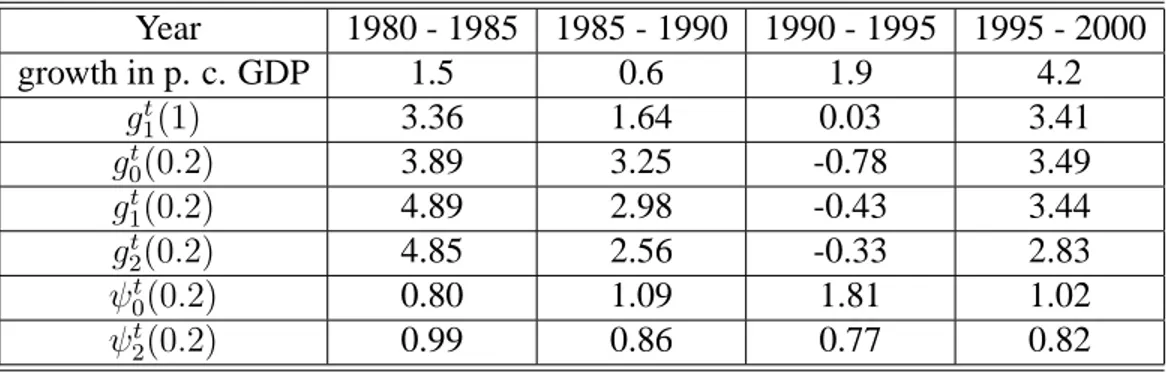
The mean consumption per capita in Tunisia grew at an annual rate (g1t(1)) of
3.36 percent between 1980 and 1985, whereas the real GDP per capita grew only by 1.5 percent. During that period indeed, oil export earnings were high, leading to high public investment in infrastructure, rapid increases in public sector wages, and generous subsidies on many foodstuffs. Table 1 shows that these policies were
highly enough pro-poor, since ψ2t(p) is very close to 1, and since the growth rate
for the less-so-poor is lower than the growth rate in the mean income of the poor (ψt0(p) = 0.8).
Unfortunately, such a pattern of growth could not be maintained since it led to a rise in the foreign debt and then to the adoption of the structural adjustment pro-gram in 1986. Although the mean consumption during 1985 – 1990 grew always at a higher rate than the real GDP per capita, gains from economic growth were not spread across the poorest as much as across the less-so-poor. Meanwhile, the
growth pattern seems to be either r-type pro-poor, as ψ0t(p) is greater than 1, or
highly enough pro-poor, as ψt2(p) > 0.66. This growth pattern also characterizes
1995 – 2000, except that it is not obtained at the risk of deteriorating macroeco-nomic imbalances.
Although really low, Table 1 reveals that growth in the mean consumption (gt1(1)) was positive between 1990 and 1995, but growth rate for the poor (g1t(0.2)) was negative. The growth pattern during that period is then pro-rich. Yet the high
value of ψ0t(p) and the weak value of ψ2t(p) let us believe that the the poorest have
Table 1: Pro-poor growth indicators Year 1980 - 1985 1985 - 1990 1990 - 1995 1995 - 2000 growth in p. c. GDP 1.5 0.6 1.9 4.2 gt 1(1) 3.36 1.64 0.03 3.41 gt 0(0.2) 3.89 3.25 -0.78 3.49 gt 1(0.2) 4.89 2.98 -0.43 3.44 gt 2(0.2) 4.85 2.56 -0.33 2.83 ψt 0(0.2) 0.80 1.09 1.81 1.02 ψt 2(0.2) 0.99 0.86 0.77 0.82
Whether these findings are robust to the choice of poverty lines and indices depends on how growth rates are distributed across the population. Figure 2 dis-plays the estimate of Tunisian’s growth incidence curve and the mean growth rate for the poorest quarter of the population. The first conclusion that may be drawn from these curves is that, with the exception of the 1990 – 1995 period, economic growth has been sufficiently spread over poor people during the last two decades. In addition, for 1980 – 1985, FOD conditions are instructive, showing that growth pattern is progressive Pen-pro-poor during the former period – at least for the poorest decile. This growth pattern leads to a two-edge impact on poverty: in-creasing substantially the income of the poor and reducing inequality within the poor, as the sharply downward trend for the 10% poorest quantiles proves, thus making the growth pattern really Pen-pro-poor.
By showing a strictly upward growth curve incidence, FOD conditions are instructive too for the second period under consideration. While undertaking the structural adjustment program during 1986 – 1991, the government did not cut back drastically on social spending. Further, Tunisia experienced a sustained per capita consumption growth of about 1.64% during the same period, as table 1 reports. Thus, economic growth, coupled with the pro-poor and redistributive policies, made the growth incidence curve taking on a logarithmic shape, with highest growth rates observed for those ranging between the 7th and the 25th percentile. Unfortunately, this progressive figure is offset by a regressive one experienced by the 7th poorest quantiles. This slowed down poverty measures decline, mainly the distribution-sensitive ones, and led to a highly enough Pen-pro-poor growth; as figure 2 illustrates.
The findings drawn from the first period and, to a lesser extent, from the sec-ond period are edifying in such a way that there is no need to test higher ethical orders for these two periods. Yet FOD conditions are much less informative for the
two last periods. While FOD conditions hold between 1995 and 2000 (g0t(p) ≥ 0
for all p), indicating that economic growth has unambiguously reduced at least absolute poverty, the slopes of the corresponding curve switch sign more than once, meaning that the extent to which growth is pro-poor critically depends on the position of the poverty line as well as on the aggregation procedure. For the
1990-1995 period however, both g0t(p) and its first derivative switch sign, which
means that neither the poverty trend, nor the growth (or recession) pattern could be appreciated using only Pen ethical criteria.
Figure 3 shows the growth deficit and severity curves for the 1990 – 1995 and 1995 – 2000. The figure also shows the extent to which growth pattern was
pro-poor. For the former period, g11995(p) (and so g21995(p)) is negative for all p, which
indicates a Dalton-increasing of poverty. Further, the corresponding curves take on an inverted U shape in the negative orthant. This indicates that the income of the poorest decreased more than that of the not-so-poor. This is confirmed by the
bottom left figure 3 which indicates that the value of ψ21995(p) is greater than 1
for the 5th poorest quantiles and greater than 0.7 for the 25th poorest quantiles. Since table 1 reveals that growth in the mean consumption was positive between 1990 and 1995, we have then an example of immiserizing growth during that period. As for the 1995 – 2000 period, the top right figure 3 shows that the 3rd poorest quantiles have experienced a regressive Dalton-pro-poor growth. This slowed down the progressive pattern of growth experienced by the less-so-poor and prevented economic growth from being unambiguously progressive
Dalton-improving. This is confirmed by the third stochastic dominance tests summarized
in the bottom right figure 2, which displays the estimates of ψ22000(p). This figure
clearly shows that growth was highly enough pro-poor since the value of ψ20002 (p)
is always greater than 0.8 for the 25th poorest quantiles and very close to 1 for the 3rd poorest quantiles.
5
Conclusion
This paper is concerned with the measurement of the extent to which economic growth (or contraction) is spread across the less well-off. For this, complete poverty orderings are first used to suggest a new index of pro-poor growth which is, contrary to Pernia and Kakwani (2000) index, in line with the usual core
ax-ioms of poverty measurement. Secondly, partial poverty orderings are used to extend the framework of Ravallion and Chen (2003) and Son (2004) to any de-gree of ethical dominance. The method can then be used to calculate the dede-gree of pro-poor growth for large classes of poverty indices and for ranges of possible poverty lines.
The empirical illustration is made using household surveys from Tunisia, cov-ering the period 1980–2000. The calculations show that the poorest quartile of the population benefit substantially enough from economic growth but lose more than the non-poor in the presence of economic contraction.
References
[1] Atkinson, A. B. (1970), On the Measurement of Inequality, Journal of Eco-nomic Theory 2, 244-263.
[2] Atkinson, A. B. (1987), On the Measurement of Poverty. Econometrica, vol. 55 (4), pp. 749-764.
[3] Bhagwati, J. N. (1988), Poverty and Public Policy. World Development, vol. 16 (5), pp. 539-554.
[4] Bibi, S. and J.-Y. Duclos (2003), Poverty Decreasing Indirect Tax Reforms: Evidence from Tunisia. CIRPEE Working Paper # 04-03.
[5] Bibi, S. and J.-Y. Duclos (2005), Decomposing Poverty Changes into Verti-cal and Horizontal Components. Bulletin of Economic Research. vol. 57 (2), pp. 205-215.
[6] Bourguignon, F. and G. S. Fields (1997), Discontinuous Losses from
Poverty, Generalized PαMeasures, and Optimal Transfers to the Poor.
Jour-nal of Public Economics, vol. 63 (2), pp. 155-175.
[7] Datt, G. and M. Ravallion (1992), Growth and Redistribution Components of Changes in Poverty: A Decomposition with Application to Brazil and India. Journal of Development Economics, vol. 38, pp. 275-295.
[8] Davidson, R., and J.-Y. Duclos (2000), Statistical Inference for Stochastic Dominance and for the Mesearement of Poverty and Inequality.
[9] Duclos,J.-Y. and P. Gr´egoire (2002), Absolute and Relative Deprivation and the Measurement of Poverty. Review of Income and Wealth, Series 48, (4), pp. 471-492.
[10] Duclos,J.-Y. and Q. Wodon (2004), What is Pro-Poor? Mimeo, CIRPEE and Laval University, Quebec, Canada.
[11] Foster, J. E., J. Greer and E. Thorbecke (1984), A Class of Decomposable Poverty Measures, Econometrica, vol. 52, 761-765.
[12] Foster, J. E. and A. Shorroks, (1988), Poverty Orderings. Econometrica, vol. 56, pp. 173-176.
[13] Hagenaars, A, (1987), A Class of Poverty Indices. International Economic
Review, vol. 28, pp. 583-607.
[14] Institut National de la Statistique (1980), Enqute Nationale sur le Budget et
la Consommation des Mnages - 1980.
[15] Institut National de la Statistique (1985), Enqute Nationale sur le Budget et
la Consommation des Mnages - 1985.
[16] Institut National de la Statistique (1990), Enqute Nationale sur le Budget et
la Consommation des Mnages - 1990.
[17] Institut National de la Statistique (1995), Enqute Nationale sur le Budget et
la Consommation, et le Niveau de Vie des Mnages - 1995.
[18] Institut National de la Statistique (2000), Enqute Nationale sur le Budget et
la Consommation, et le Niveau de Vie des Mnages - 2000.
[19] Kakwani, N. (1980), On a Class of Poverty Measures. Econometrica, vol. 48, pp. 437-46.
[20] Kakwani, N. and E. M. Pernia (2000), What is Pro-poor Growth? Asian
Development Review, vol. 18 (1), pp. 1-16.
[21] Kraay, A. (2004), When is Growth Pro-Poor? Evidence from a Panel of Countries. Forthcoming in Journal of Development Economics.
[23] Ravallion, M. and S. Chen (2003), Measuring Pro-Poor Growth. Economics
Letters, vol. 78, pp. 93-99.
[24] Rawls, J. (1971), A Theory of Justice. Cambridge, Massachusetts, Havard University Press.
[25] Sen, A. K. (1976), Poverty: An Ordinal Approach to Measurement.
Econo-metrica, vol. 44 (2), pp. 219-231.
[26] Silverman, B. W. (1986), Density Estimation for Statistics and Data
Analy-sis. Chapman and Hall, London.
[27] Son, H. H. (2004), A Note on Measuring Pro-Poor Growth. Economics
Let-ters, vol. 82 (3), pp. 307-314.
[28] Takayama, N. (1979), Poverty, Income Inequality, and their Measures: Pro-fessor sen’s Axiomatic Approach Reconsidered. Econometrica, vol. 47, pp. 747-759.
[29] UNDP (1999), Republic of Tunisia: National Report on Human
Develop-ment.
[30] World Bank (1995) Republic of Tunisia, Poverty Alleviation: Preserving Progress while Preparing for the Future. Middle East and North Africa
Re-gion, Report N◦13993-TUN.
[31] World Bank (1999), Rpublique Tunisienne, Revue Sociale et Structurelle. Unpublished work.
Figure 1: Non-parametric Estimation of some Distrib utions Function 0 .2 .4 .6 Density 4 6 8 10 LRBT
Great Tunis Distribution
0 .2 .4 .6 Density 4 6 8 10 LRBT
North Distribution
0 .2 .4 .6 Density 4 5 6 7 8 9 LRBTCenter Distribution
0 .2 .4 .6 Density 4 6 8 10 LRBTSouth Distribution
Figure 2: Pen-Pro-poor Gro wth 4 6 8 1012 Growth rate 0 5 10 15 20 25 Percentile g0_85 mean_g0_85
1980 − 1985
1.5 2 2.5 3 3.5 Growth rate 0 5 10 15 20 25 Percentile g0_90 mean_g0_901985 − 1990
−2 −1.5 −1−.5 0 .5 Growth rate 0 5 10 15 20 25 Percentile g0_95 mean_g0_951990 − 1995
33.5 44.5 55.5 Growth rate 0 5 10 15 20 25 Percentile g0_00 mean_g0_001995 − 2000
Figure 3: Dalton-Pro-poor Gro wth and De gree of Pro-poor Gro wth −1.5 −1 −.5 0 Growth rate 0 5 10 15 20 25 Percentile g1_95 g2_95
1990 − 1995
3 3.5 4 4.5 5 Growth rate 0 5 10 15 20 25 Percentile g1_00 g2_001995 − 2000
.8 1 1.2 1.4 1.6Pro−poor growth ratio
0 5 10 15 20 25 Percentile
Pro−poor growth 1990 − 1995
.8 .85 .9 .95 1Pro−poor growth ratio
0 5 10 15 20 25 Percentile