Algorithms and Ordering Heuristics for Distributed Constraint Satisfaction Problems

Texte intégral

(1)Algorithms and Ordering Heuristics for Distributed Constraint Satisfaction Problems Mohamed Wahbi. To cite this version: Mohamed Wahbi. Algorithms and Ordering Heuristics for Distributed Constraint Satisfaction Problems. Artificial Intelligence [cs.AI]. Université Montpellier II - Sciences et Techniques du Languedoc; Université Mohammed V-Agdal, Rabat, 2012. English. �tel-00718537v2�. HAL Id: tel-00718537 https://tel.archives-ouvertes.fr/tel-00718537v2 Submitted on 27 Aug 2012. HAL is a multi-disciplinary open access archive for the deposit and dissemination of scientific research documents, whether they are published or not. The documents may come from teaching and research institutions in France or abroad, or from public or private research centers.. L’archive ouverte pluridisciplinaire HAL, est destinée au dépôt et à la diffusion de documents scientifiques de niveau recherche, publiés ou non, émanant des établissements d’enseignement et de recherche français ou étrangers, des laboratoires publics ou privés..

(2) LIRMM. Université Montpellier 2. Université Mohammed V - Agdal. Sciences et Techniques du Languedoc France. Faculté des Sciences du Rabat Maroc. Ph.D Thesis présentée pour obtenir le diplôme de Doctorat en Informatique de l’Université Montpellier 2 & l’Université Mohammed V-Agdal par. Mohamed Wahbi Spécialité : Informatique École Doctorale Information, Structures, Systèmes- France & Le Centre d’Etudes Doctorales en Sciences et Technologies de Rabat- Maroc. Algorithms and Ordering Heuristics for Distributed Constraint Satisfaction Problems. Soutenue le 03 Juillet 2012, devant le jury composé de :. President Mme. Awatef Sayah, PES . . . . . . . . . . . . . . . . . . . . . . . . Université Mohammed V-Agdal, Maroc Reviewers Mr. Pedro Meseguer, Directeur de recherche . . . . . . . . . . . . . . . . . . . . IIIA, Barcelona, Espagne Mr. Mustapha Belaissaoui, Professeur Habilité . . . . . l’ENCG, Université Hassan I, Maroc Examinator Mr. Rémi Coletta, Maitre de conférence . . . . . . . LIRMM, Université Montpellier 2, France Supervisors Mr. Christian Bessiere, Directeur de recherche . LIRMM, Université Montpellier 2, France Mr. El Houssine Bouyakhf, PES . . . . . . . . . . . . . . . . . . Université Mohammed V-Agdal, Maroc.

(3)

(4) iii. To my family.

(5)

(6) Acknowledgements. The research work presented in this thesis has been performed in the Laboratoire d’Informatique Mathématiques appliquées Intelligence Artificielle et Reconnaissance de Formes (LIMIARF), Faculty of Science, University Mohammed V-Agdal, Rabat, Morocco and the Laboratoire d’Informatique, de Robotique et de Microélectronique de Montpellier (LIRMM), University Montpellier 2, France. This thesis has been done in collaboration between University Mohammed V-Agdal, Morocco and University Montpellier 2, France under the financial support of the scholarship of the programme Averroés funded by the European Commission within the framework of Erasmus Mundus. First and foremost, it is with immense gratitude that I acknowledge all the support, advice, and guidance of my supervisors, Professor El-Houssine Bouyakhf and Dr. Christian Bessiere. It was a real pleasure to work with them. Their truly scientist intuition has made them as a source of ideas and passions in science, which exceptionally inspire and enrich my growth as a student, a researcher and a scientist want to be. I want to thank them especially for letting me wide autonomy while providing appropriate advice. I am indebted to them more than they know and hope to keep up our collaboration in the future. I gratefully acknowledge Professor Awatef Sayah (Faculty of sciences, University Mohammed V-Agdal, Morocco) for accepting to preside the jury of my dissertation. I am most grateful to my reviewers Professor Pedro Meseguer (Scientific Researcher, the Artificial Intelligence Research Institute (IIIA), Barcelona, Spain) and Professor Mustapha Belaissaoui (Professeur Habilité, ENCG, University Hassan I, Morocco) for their constructive comments on this thesis. I am thankful that in the midst of all their activities, they accepted to review my thesis. I would like to record my gratitude to Professor Rémi Coletta, (Maître de conférence, University Montpellier 2, France) for his thorough examination of the thesis. Many of the works published during this thesis have been done in collaboration with so highly motivated, smart, enthusiastic, and passionate coauthors. I want to thank them for their teamwork, talent, hard work and devotion. I cannot thank my coauthors without giving my special gratefulness to Professor Redouane Ezzahir and Doctor Younes Mechqrane. I thank the great staffs of the LIRMM and LIMIARF Laboratories for the use of facilities, consultations and moral support. The LIRMM has provided the support and equipment I have needed to produce and complete my thesis. I also want to thank my colleagues at the LIRMM and LIMIARF Laboratories for the joyful and pleasant working environment. v.

(7) vi. Acknowledgements. Especially, I would like to thank the members of the Coconut/LIRMM and IA/LIMIARF teams. I acknowledge Amine B., Fabien, Eric, Imade, Saida, Fred, Philippe, Brahim and Jaouad. In my daily work I have been blessed with a friendly and cheerful group of fellow students. I would like to particularly thank Hajer, Younes, Mohamed, Kamel, Nawfal, Mohammed, Nabil Z., Farid, Azhar, Kaouthar, Samir, Nabil Kh., Amine M., and Hassan. It is a pleasure to express my gratitude wholeheartedly to Baslam’s family for their kind hospitality during my stay in Montpellier. Further, I am also very thankful to the professors of the department of Computer Science, University Montpellier 2, with whom I have been involved as a temporary assistant professor (Attaché Temporaire d’Enseignement et de Recherche - ATER) for providing an excellent environment to teach and develop new pedagogical techniques. I convey special acknowledgment to Professor Marianne Huchard. Most importantly, words alone cannot express the thanks I owe to my family for believing and loving me, especially my mother who has always filled my life with generous love, and unconditional support and prayers. My thanks go also to my lovely sister and brother, my uncles and antes and all my family for their endless moral support throughout my career. To them I dedicate this thesis. Last but not the least, the one above all of us, the omnipresent God, for answering my prayers for giving me the strength to plod on despite my constitution wanting to give up and throw in the towel, thank you so much Dear Lord. Finally, I would like to thank everybody who was important to the successful realization of thesis, as well as expressing my apology that I could not mention personally one by one.. Montpellier, July 3rd , 2012. Mohamed Wahbi.

(8) Abstract. Distributed Constraint Satisfaction Problems (DisCSP) is a general framework for solving distributed problems. DisCSP have a wide range of applications in multi-agent coordination. In this thesis, we extend the state of the art in solving the DisCSPs by proposing several algorithms. Firstly, we propose the Nogood-Based Asynchronous Forward Checking (AFC-ng), an algorithm based on Asynchronous Forward Checking (AFC). However, instead of using the shortest inconsistent partial assignments, AFC-ng uses nogoods as justifications of value removals. Unlike AFC, AFC-ng allows concurrent backtracks to be performed at the same time coming from different agents having an empty domain to different destinations. Then, we propose the Asynchronous Forward-Checking Tree (AFCtree). In AFC-tree, agents are prioritized according to a pseudo-tree arrangement of the constraint graph. Using this priority ordering, AFC-tree performs multiple AFC-ng processes on the paths from the root to the leaves of the pseudo-tree. Next, we propose to maintain arc consistency asynchronously on the future agents instead of only maintaining forward checking. Two new synchronous search algorithms that maintain arc consistency asynchronously (MACA) are presented. After that, we developed the Agile Asynchronous Backtracking (Agile-ABT), an asynchronous dynamic ordering algorithm that does not follow the standard restrictions in asynchronous backtracking algorithms. The order of agents appearing before the agent receiving a backtrack message can be changed with a great freedom while ensuring polynomial space complexity. Next, we present a corrigendum of the protocol designed for establishing the priority between orders in the asynchronous backtracking algorithm with dynamic ordering using retroactive heuristics (ABT_DO-Retro). Finally, the new version of the DisChoco open-source platform for solving distributed constraint reasoning problems is described. The new version is a complete redesign of the DisChoco platform. DisChoco 2.0 is an open source Java library which aims at implementing distributed constraint reasoning algorithms. Keywords: Distributed Artificial Intelligence, Distributed Constraint Satisfaction (DisCSP), Distributed Solving, Maintaining Arc Consistency, Reordering, DisChoco.. vii.

(9)

(10) Résumé. Les problèmes de satisfaction de contraintes distribués (DisCSP) permettent de formaliser divers problèmes qui se situent dans l’intelligence artificielle distribuée. Ces problèmes consistent à trouver une combinaison cohérente des actions de plusieurs agents. Durant cette thèse nous avons apporté plusieurs contributions dans le cadre des DisCSPs. Premièrement, nous avons proposé le Nogood-Based Asynchronous Forward-Checking (AFCng). Dans AFC-ng, les agents utilisent les nogoods pour justifier chaque suppression d’une valeur du domaine de chaque variable. Outre l’utilisation des nogoods, plusieurs backtracks simultanés venant de différents agents vers différentes destinations sont autorisés. En deuxième lieu, nous exploitons les caractéristiques intrinsèques du réseau de contraintes pour exécuter plusieurs processus de recherche AFC-ng d’une manière asynchrone à travers chaque branche du pseudo-arborescence obtenu à partir du graphe de contraintes dans l’algorithme Asynchronous Forward-Checking Tree (AFC-tree). Puis, nous proposons deux nouveaux algorithmes de recherche synchrones basés sur le même mécanisme que notre AFC-ng. Cependant, au lieu de maintenir le forward checking sur les agents non encore instanciés, nous proposons de maintenir la consistance d’arc. Ensuite, nous proposons Agile Asynchronous Backtracking (Agile-ABT), un algorithme de changement d’ordre asynchrone qui s’affranchit des restrictions habituelles des algorithmes de backtracking asynchrone. Puis, nous avons proposé une nouvelle méthode correcte pour comparer les ordres dans ABT_DO-Retro. Cette méthode détermine l’ordre le plus pertinent en comparant les indices des agents dès que les compteurs d’une position donnée dans le timestamp sont égaux. Finalement, nous présentons une nouvelle version entièrement restructurée de la plateforme DisChoco pour résoudre les problèmes de satisfaction et d’optimisation de contraintes distribués. Mots clefs : L’intelligence artificielle distribuée, les problèmes de satisfaction de contraintes distribués (DisCSP), la résolution distribuée, la maintenance de la consistance d’arc, les heuristiques ordonnancement, DisChoco.. ix.

(11)

(12) Contents. Acknowledgements. v. Abstract (English/Français). vii. Contents. xi 1. Introduction 1. Background 1.1 Centralized Constraint Satisfaction Problems (CSP) . . . . . . . . . . 1.1.1 Preliminaries . . . . . . . . . . . . . . . . . . . . . . . . . . . . 1.1.2 Examples of CSPs . . . . . . . . . . . . . . . . . . . . . . . . . 1.1.2.1 The n-queens problem . . . . . . . . . . . . . . . . . 1.1.2.2 The Graph Coloring Problem . . . . . . . . . . . . . 1.1.2.3 The Meeting Scheduling Problem . . . . . . . . . . . 1.2 Algorithms and Techniques for Solving Centralized CSPs . . . . . . 1.2.1 Algorithms for solving centralized CSPs . . . . . . . . . . . . 1.2.1.1 Chronological Backtracking (BT) . . . . . . . . . . . 1.2.1.2 Conflict-directed Backjumping (CBJ) . . . . . . . . . 1.2.1.3 Dynamic Backtracking (DBT) . . . . . . . . . . . . . 1.2.1.4 Partial Order Dynamic Backtracking (PODB) . . . . 1.2.1.5 Forward Checking (FC) . . . . . . . . . . . . . . . . . 1.2.1.6 Arc-consistency (AC) . . . . . . . . . . . . . . . . . . 1.2.1.7 Maintaining Arc-Consistency (MAC) . . . . . . . . . 1.2.2 Variable Ordering Heuristics for Centralized CSP . . . . . . . 1.2.2.1 Static Variable Ordering Heuristics (SVO) . . . . . . 1.2.2.2 Dynamic Variable Ordering Heuristics (DVO) . . . . 1.3 Distributed constraint satisfaction problems (DisCSP) . . . . . . . . . 1.3.1 Preliminaries . . . . . . . . . . . . . . . . . . . . . . . . . . . . 1.3.2 Examples of DisCSPs . . . . . . . . . . . . . . . . . . . . . . . 1.3.2.1 Distributed Meeting Scheduling Problem (DisMSP) 1.3.2.2 Distributed Sensor Network Problem (SensorDCSP) 1.4 Methods for solving distributed CSPs . . . . . . . . . . . . . . . . . . 1.4.1 Synchronous search algorithms on DisCSPs . . . . . . . . . . 1.4.1.1 Asynchronous Forward-Checking (AFC) . . . . . . . 1.4.2 Asynchronous search algorithms on DisCSPs . . . . . . . . .. . . . . . . . . . . . . . . . . . . . . . . . . . . .. . . . . . . . . . . . . . . . . . . . . . . . . . . .. . . . . . . . . . . . . . . . . . . . . . . . . . . .. . . . . . . . . . . . . . . . . . . . . . . . . . . .. . . . . . . . . . . . . . . . . . . . . . . . . . . .. 7 7 9 10 10 11 11 13 14 15 16 18 19 20 21 23 23 24 25 28 29 30 31 32 33 34 35 37 xi.

(13) 1.5 2. 3. 4. xii. 1.4.2.1 Asynchronous Backtracking (ABT) 1.4.3 Dynamic Ordering Heuristics on DisCSPs . 1.4.4 Maintaining Arc Consistency on DisCSPs . . Summary . . . . . . . . . . . . . . . . . . . . . . . . .. . . . .. . . . .. Nogood based Asynchronous Forward Checking (AFC-ng) 2.1 Introduction . . . . . . . . . . . . . . . . . . . . . . . . . 2.2 Nogood-based Asynchronous Forward Checking . . . 2.2.1 Description of the algorithm . . . . . . . . . . . 2.3 Correctness Proofs . . . . . . . . . . . . . . . . . . . . . 2.4 Experimental Evaluation . . . . . . . . . . . . . . . . . . 2.4.1 Uniform binary random DisCSPs . . . . . . . . 2.4.2 Distributed Sensor Target Problems . . . . . . . 2.4.3 Distributed Meeting Scheduling Problems . . . 2.4.4 Discussion . . . . . . . . . . . . . . . . . . . . . . 2.5 Other Related Works . . . . . . . . . . . . . . . . . . . . 2.6 Summary . . . . . . . . . . . . . . . . . . . . . . . . . . . Asynchronous Forward Checking Tree (AFC-tree) 3.1 Introduction . . . . . . . . . . . . . . . . . . . . . . 3.2 Pseudo-tree ordering . . . . . . . . . . . . . . . . . 3.3 Distributed Depth-First Search trees construction 3.4 The AFC-tree algorithm . . . . . . . . . . . . . . . 3.4.1 Description of the algorithm . . . . . . . . 3.5 Correctness Proofs . . . . . . . . . . . . . . . . . . 3.6 Experimental Evaluation . . . . . . . . . . . . . . . 3.6.1 Uniform binary random DisCSPs . . . . . 3.6.2 Distributed Sensor Target Problems . . . . 3.6.3 Distributed Meeting Scheduling Problems 3.6.4 Discussion . . . . . . . . . . . . . . . . . . . 3.7 Other Related Works . . . . . . . . . . . . . . . . . 3.8 Summary . . . . . . . . . . . . . . . . . . . . . . . .. . . . . . . . . . . . . .. . . . . . . . . . . . . .. . . . . . . . . . . . . .. . . . .. . . . . . . . . . . .. . . . . . . . . . . . . .. . . . .. . . . . . . . . . . .. . . . . . . . . . . . . .. . . . .. . . . . . . . . . . .. . . . . . . . . . . . . .. . . . .. . . . . . . . . . . .. . . . . . . . . . . . . .. . . . .. . . . . . . . . . . .. . . . . . . . . . . . . .. . . . .. . . . . . . . . . . .. . . . . . . . . . . . . .. . . . .. . . . . . . . . . . .. . . . . . . . . . . . . .. . . . .. . . . . . . . . . . .. . . . . . . . . . . . . .. . . . .. . . . . . . . . . . .. . . . . . . . . . . . . .. . . . .. . . . . . . . . . . .. . . . . . . . . . . . . .. . . . .. . . . . . . . . . . .. . . . . . . . . . . . . .. . . . .. . . . . . . . . . . .. . . . . . . . . . . . . .. . . . .. 37 42 43 43. . . . . . . . . . . .. 45 46 47 47 51 52 52 55 56 58 59 59. . . . . . . . . . . . . .. 61 62 63 64 67 68 70 70 71 73 74 76 76 76. Maintaining Arc Consistency Asynchronously in Synchronous Distributed Search 4.1 Introduction . . . . . . . . . . . . . . . . . . . . . . . . . . . . . . . . . . . . . . 4.2 Maintaining Arc Consistency . . . . . . . . . . . . . . . . . . . . . . . . . . . . 4.3 Maintaining Arc Consistency Asynchronously . . . . . . . . . . . . . . . . . . 4.3.1 Enforcing AC using del messages (MACA-del) . . . . . . . . . . . . . 4.3.2 Enforcing AC without additional kind of message (MACA-not) . . . . 4.4 Theoretical analysis . . . . . . . . . . . . . . . . . . . . . . . . . . . . . . . . . . 4.5 Experimental Results . . . . . . . . . . . . . . . . . . . . . . . . . . . . . . . . . 4.5.1 Discussion . . . . . . . . . . . . . . . . . . . . . . . . . . . . . . . . . . . 4.6 Summary . . . . . . . . . . . . . . . . . . . . . . . . . . . . . . . . . . . . . . . .. 77 78 79 79 80 83 84 85 87 88.

(14) 5. 6. 7. Agile Asynchronous BackTracking (Agile-ABT) 5.1 Introduction . . . . . . . . . . . . . . . . . . . 5.2 Introductory Material . . . . . . . . . . . . . . 5.2.1 Reordering details . . . . . . . . . . . 5.2.2 The Backtracking Target . . . . . . . . 5.2.3 Decreasing termination values . . . . 5.3 The Algorithm . . . . . . . . . . . . . . . . . . 5.4 Correctness and complexity . . . . . . . . . . 5.5 Experimental Results . . . . . . . . . . . . . . 5.5.1 Uniform binary random DisCSPs . . 5.5.2 Distributed Sensor Target Problems . 5.5.3 Discussion . . . . . . . . . . . . . . . . 5.6 Related Works . . . . . . . . . . . . . . . . . . 5.7 Summary . . . . . . . . . . . . . . . . . . . . .. . . . . . . . . . . . . .. . . . . . . . . . . . . .. . . . . . . . . . . . . .. . . . . . . . . . . . . .. . . . . . . . . . . . . .. . . . . . . . . . . . . .. . . . . . . . . . . . . .. . . . . . . . . . . . . .. . . . . . . . . . . . . .. . . . . . . . . . . . . .. . . . . . . . . . . . . .. . . . . . . . . . . . . .. . . . . . . . . . . . . .. Corrigendum to “Min-domain retroactive ordering for Asynchronous ing” 6.1 Introduction . . . . . . . . . . . . . . . . . . . . . . . . . . . . . . . . 6.2 Background . . . . . . . . . . . . . . . . . . . . . . . . . . . . . . . . 6.3 ABT_DO-Retro May Not Terminate . . . . . . . . . . . . . . . . . . 6.4 The Right Way to Compare Orders . . . . . . . . . . . . . . . . . . . 6.5 Summary . . . . . . . . . . . . . . . . . . . . . . . . . . . . . . . . . . DisChoco 2.0 7.1 Introduction . . . . . . . . . . . 7.2 Architecture . . . . . . . . . . . 7.2.1 Communication System 7.2.2 Event Management . . . 7.2.3 Observers in layers . . . 7.3 Using DisChoco 2.0 . . . . . . . 7.4 Experimentations . . . . . . . . 7.5 Conclusion . . . . . . . . . . . .. . . . . . . . .. . . . . . . . .. . . . . . . . .. . . . . . . . .. . . . . . . . .. . . . . . . . .. . . . . . . . .. . . . . . . . .. . . . . . . . .. . . . . . . . .. . . . . . . . .. . . . . . . . .. . . . . . . . .. . . . . . . . .. . . . . . . . .. . . . . . . . .. . . . . . . . .. . . . . . . . .. . . . . . . . .. . . . . . . . .. . . . . . . . .. . . . . . . . . . . . . .. . . . . . . . . . . . . .. . . . . . . . . . . . . .. . . . . . . . . . . . . .. . . . . . . . . . . . . .. . . . . . . . . . . . . .. 89 90 91 91 93 94 95 98 100 101 103 105 106 106. Backtrack. . . . .. . . . . . . . .. . . . . .. . . . . . . . .. . . . . .. . . . . . . . .. . . . . .. . . . . . . . .. . . . . .. . . . . . . . .. . . . . .. 107 107 108 110 112 114. . . . . . . . .. 115 115 116 117 118 118 119 121 123. Conclusions and perspectives. 125. Bibliography. 129. List of Figures. 139. List of Tables. 141. List of algorithms. 143. xiii.

(15)

(16) Introduction. Constraint programming is an area in computer science that has gained increasing interest in the last four recent decades. Constraint programming is based on its powerful framework named Constraint Satisfaction Problem (CSP). A constraint satisfaction problem is a general framework that can formalize many real world combinatorial problems. Various problems in artificial intelligence can be naturally modeled as CSPs. Therefore, the CSP paradigm has been widely used for solving such problems. Examples of these problems can inherent from various areas related to resource allocation, scheduling, logistics and planning. Solving a constraint satisfaction problem (CSP) consists in looking for solutions to a constraint network, that is, a set of assignments of values to variables that satisfy the constraints of the problem. These constraints represent restrictions on values combinations allowed for constrained variables. Numerous powerful algorithms were designed for solving constraint satisfaction problems. Typical systematic search algorithms try to construct a solution to a CSP by incrementally instantiating the variables of the problem. However, proving the existence of solutions or finding these solutions in CSP are NP-complete tasks. Thus, many heuristics were developed to improve the efficiency of search algorithms. Sensor networks [Jung et al., 2001; Béjar et al., 2005], military unmanned aerial vehicles teams [Jung et al., 2001], distributed scheduling problems [Wallace and Freuder, 2002; Maheswaran et al., 2004], distributed resource allocation problems [Petcu and Faltings, 2004], log-based reconciliation [Chong and Hamadi, 2006], Distributed Vehicle Routing Problems [Léauté and Faltings, 2011], etc. are real applications of a distributed nature, that is, knowledge is distributed among several physical distributed entities. These applications can be naturally modeled and solved by a CSP process once the knowledge about the whole problem is delivered to a centralized solver. However, in such applications, gathering the whole knowledge into a centralized solver is undesirable. In general, this restriction is mainly due to privacy and/or security requirements: constraints or possible values may be strategic information that should not be revealed to others agents that can be seen as competitors. The cost or the inability of translating all information to a single format may be another reason. In addition, a distributed system provides fault tolerance, which means that if some agents disconnect, a solution might be available for the connected part. Thereby, a distributed model allowing a decentralized solving process is more adequate. The Distributed Constraint Satisfaction Problem (DisCSP) has such properties. A distributed constraint satisfaction problem (DisCSP) is composed of a group of autonomous agents, where each agent has control of some elements of information about the whole problem, that is, variables and constraints. Each agent owns its local constraint network. Variables in different agents are connected by constraints. In order to solve a 1.

(17) Introduction. 2. DisCSP, agents must assign values to their variables so that all constraints are satisfied. Hence, agents assign values to their variables, attempting to generate a locally consistent assignment that is also consistent with constraints between agents [Yokoo et al., 1998; Yokoo, 2000a]. To achieve this goal, agents check the value assignments to their variables for local consistency and exchange messages among them to check consistency of their proposed assignments against constraints that contain variables that belong to others agents. In solving DisCSPs, agents exchange messages about the variable assignments and conflicts of constraints. Several distributed algorithms for solving DisCSPs have been designed in the last two decades. They can be divided into two main groups: asynchronous and synchronous algorithms. The first category are algorithms in which the agents assign values to their variables in a synchronous, sequential way. The second category are algorithms in which the process of proposing values to the variables and exchanging these proposals is performed asynchronously between the agents. In the former category, agents do not have to wait for decisions of others, whereas, in general only one agent has the privilege of making a decision in the synchronous algorithms.. Contributions A major motivation for research on distributed constraint satisfaction problem (DisCSP) is that it is an elegant model for many every day combinatorial problems that are distributed by nature. By the way, DisCSP is a general framework for solving various problems arising in Distributed Artificial Intelligence. Improving the efficiency of existing algorithms for solving DisCSP is a central key for research on DisCSPs. In this thesis, we extend the state of the art in solving the DisCSPs by proposing several algorithms. We believe that these algorithms are significant as they improve the current state-of-the-art in terms of runtime and number of exchanged messages experimentally. Nogood-Based Asynchronous Forward Checking (AFC-ng) is an asynchronous algorithm based on Asynchronous Forward Checking (AFC) for solving DisCSPs. Instead of using the shortest inconsistent partial assignments AFC-ng uses nogoods as justifications of value removals. Unlike AFC, AFC-ng allows concurrent backtracks to be performed at the same time coming from different agents having an empty domain to different destinations. Thanks to the timestamps integrated in the CPAs, the strongest CPA coming from the highest level in the agent ordering will eventually dominate all others. Interestingly, the search process with the strongest CPA will benefit from the computational effort done by the (killed) lower level processes. This is done by taking advantage from nogoods recorded when processing these lower level processes. Asynchronous Forward-Checking Tree (AFC-tree) The main feature of the AFC-tree algorithm is using different agents to search non-intersecting parts of the search space concurrently. In AFC-tree, agents are prioritized according to a pseudo-tree arrangement of the constraint graph. The pseudo-tree ordering is built in a preprocessing step. Using this priority ordering, AFC-tree performs multiple AFC-ng processes on the paths from the root to the leaves of the pseudo-tree. The agents that are brothers.

(18) Introduction. are committed to concurrently find the partial solutions of their variables. Therefore, AFC-tree exploits the potential speed-up of a parallel exploration in the processing of distributed problems. Maintaining Arc Consistency Asynchronously (MACA) Instead of maintaining forward checking asynchronously on agents not yet instantiated, as is done in AFC-ng, we propose to maintain arc consistency asynchronously on these future agents. We propose two new synchronous search algorithms that maintain arc consistency asynchronously (MACA). The first algorithm we propose, MACA-del, enforces arc consistency thanks to an additional type of messages, deletion messages (del). Hence, whenever values are removed during a constraint propagation step, MACA-del agents notify others agents that may be affected by these removals, sending them a del message. The second algorithm, MACA-not, achieves arc consistency without any new type of message. We achieve this by storing all deletions performed by an agent on domains of its neighboring agents, and sending this information to these neighbors within the CPA message. Agile Asynchronous Backtracking (Agile-ABT) is an asynchronous dynamic ordering algorithm that does not follow the standard restrictions in asynchronous backtracking algorithms. The order of agents appearing before the agent receiving a backtrack message can be changed with a great freedom while ensuring polynomial space complexity. Furthermore, that agent receiving the backtrack message, called the backtracking target, is not necessarily the agent with the lowest priority within the conflicting agents in the current order. The principle of Agile-ABT is built on termination values exchanged by agents during search. A termination value is a tuple of positive integers attached to an order. Each positive integer in the tuple represents the expected current domain size of the agent in that position in the order. Orders are changed by agents without any global control so that the termination value decreases lexicographically as the search progresses. Since a domain size can never be negative, termination values cannot decrease indefinitely. An agent informs the others of a new order by sending them its new order and its new termination value. When an agent compares two contradictory orders, it keeps the order associated with the smallest termination value. Corrigendum to “Min-domain retroactive ordering for Asynchronous Backtracking”: A corrigendum of the protocol designed for establishing the priority between orders in the asynchronous backtracking algorithm with dynamic ordering using retroactive heuristics (ABT_DO-Retro). We presented an example that shows how ABT_DO-Retro can enter an infinite loop following the natural understanding of the description given by the authors of ABT_DO-Retro. We describe the correct way for comparing time-stamps of orders. We give the proof that our method for comparing orders is correct. DisChoco 2.0: is open-source platform for solving distributed constraint reasoning problems. The new version 2.0 is a complete redesign of the DisChoco platform. DisChoco. 3.

(19) Introduction. 4. 2.0 is not a distributed version of the centralized solver Choco 1 , but it implements a model to solve distributed constraint networks with local complex problems (i.e., several variables per agent) by using Choco as local solver to each agent. The novel version we propose contains several interesting features: it is reliable and modular, it is easy to personalize and to extend, it is independent from the communication system and allows a deployment in a real distributed system as well as the simulation on a single Java Virtual Machine. DisChoco 2.0 is an open source Java library which aims at implementing distributed constraint reasoning algorithms from an abstract model of agent (already implemented in DisChoco). A single implementation of a distributed constraint reasoning algorithm can run as simulation on a single machine, or on a network of machines that are connected via the Internet or via a wireless ad-hoc network, or even on mobile phones compatible with J2ME.. Thesis Outline Chapter 1 introduces the state of the art in the area of centralized and distributed constraint programming. We define the constraint satisfaction problem formalism (CSP) and present some academic and real examples of problems that can be modeled and solved by CSP. We then briefly present typical methods for solving centralized CSP. Next, we give preliminary definitions on the distributed constraint satisfaction problem paradigm (DisCSP). Afterwards we describe the main algorithms that have been developed in the literature to solve DisCSPs. We present our first contribution, the Nogood-Based of Asynchronous Forward Checking (AFC-ng), in Chapter 2. Besides its use of nogoods as justification of value removals, AFC-ng allows simultaneous backtracks to go from different agents to different destinations. We prove that AFC-ng only needs polynomial space. Correctness proofs of the AFC-ng are also given. We compare the performance of our algorithm against others well-known distributed algorithms for solving DisCSP. We present the results on random DisCSPs and instances from real benchmarks: sensor networks and distributed meeting scheduling. In Chapter 3, we show how to extend our nogood-based Asynchronous ForwardChecking (AFC-ng) algorithm to the Asynchronous Forward-Checking Tree (AFC-tree) algorithm using a pseudo-tree arrangement of the constraint graph. To achieve this goal, agents are ordered a priory in a pseudo-tree such that agents in different branches of the tree do not share any constraint. AFC-tree does not address the process of ordering the agents in a pseudo-tree arrangement. Therefore, the construction of the pseudo-tree is done in a preprocessing step. We demonstrate the good properties of the Asynchronous Forward-Checking Tree. We provide a comparison of our AFC-tree to the AFC-ng on random DisCSPs and instances from real benchmarks: sensor networks and distributed meeting scheduling. Chapter 4 presents the first attempt to maintain the arc consistency in the synchronous 1. http://choco.emn.fr/.

(20) Introduction. search algorithm. Indeed, instead of using forward checking as a filtering property like AFC-ng we propose to maintain arc consistency asynchronously (MACA). Thus, we propose two new algorithms based on the same mechanism as AFC-ng that enforce arc consistency asynchronously. The first algorithm we propose, MACA-del, enforces arc consistency thanks to an additional type of messages, deletion messages. The second algorithm, MACA-not, achieves arc consistency without any new type of message. We provide a theoretical analysis and an experimental evaluation of the proposed approach. Chapter 5 proposes Agile Asynchronous Backtracking algorithm (Agile-ABT), a search procedure that is able to change the ordering of agents more than previous approaches. This is done via the original notion of termination value, a vector of stamps labeling the new orders exchanged by agents during search. We first describe the concepts needed to select new orders that decrease the termination value. Next, we give the details of our algorithm and we show how agents can reorder themselves as much as they want as long as the termination value decreases as the search progresses. We also prove Agile-ABT in Chapter 5. An experimental evaluation is provided by the end of this chapter. Chapter 6 provides a corrigendum of the protocol designed for establishing the priority between orders in the asynchronous backtracking algorithm with dynamic ordering using retroactive heuristics (ABT_DO-Retro). We illustrate in this chapter an example that shows, if ABT_DO-Retro uses that protocol, how it can fall into an infinite loop. We present the correct method for comparing time-stamps and give the proof that our method for comparing orders is correct. Finally, in Chapter 7, we describe our distributed constraint reasoning platform DisChoco 2.0. DisChoco is an open-source framework that provides a simple implementation of all these algorithms and obviously many other. DisChoco 2.0 then offers a complete tool for the research community for evaluating algorithms performance or being used for real applications.. 5.

(21)

(22) 1. Background. Contents 3.1. Introduction . . . . . . . . . . . . . . . . . . . . . . . . . . . . . . . . . . . . . . . . . .. 62. 3.2. Pseudo-tree ordering . . . . . . . . . . . . . . . . . . . . . . . . . . . . . . . . . . . .. 63. 3.3. Distributed Depth-First Search trees construction . . . . . . . . . . . . . . . . .. 64. 3.4. The AFC-tree algorithm . . . . . . . . . . . . . . . . . . . . . . . . . . . . . . . . . . .. 67. Description of the algorithm . . . . . . . . . . . . . . . . . . . . . . . . . . . . .. 68. 3.5. Correctness Proofs . . . . . . . . . . . . . . . . . . . . . . . . . . . . . . . . . . . . . .. 70. 3.6. Experimental Evaluation . . . . . . . . . . . . . . . . . . . . . . . . . . . . . . . . . .. 70. 3.6.1. Uniform binary random DisCSPs . . . . . . . . . . . . . . . . . . . . . . . . . .. 71. 3.6.2. Distributed Sensor Target Problems . . . . . . . . . . . . . . . . . . . . . . . . .. 73. 3.6.3. Distributed Meeting Scheduling Problems . . . . . . . . . . . . . . . . . . . . .. 74. 3.6.4. Discussion . . . . . . . . . . . . . . . . . . . . . . . . . . . . . . . . . . . . . . . .. 76. 3.7. Other Related Works . . . . . . . . . . . . . . . . . . . . . . . . . . . . . . . . . . . .. 76. 3.8. Summary . . . . . . . . . . . . . . . . . . . . . . . . . . . . . . . . . . . . . . . . . . . . .. 76. 3.4.1. T. his chapter introduces the state of the art in the area of centralized and distributed constraint programming. In Section 1.1 we define the constraint satisfaction problem formalism (CSP) and present some academic and real examples of problems modeled and solved by CSPs. Typical methods for solving centralized CSP are presented in Section 1.2. Next, we give preliminary definitions on the distributed constraint satisfaction problem paradigm (DisCSP) in Section 1.3. The state of the art algorithms and heuristic for solving DisCSPs are provided in Section 1.4.. 1.1 Centralized Constraint Satisfaction Problems (CSP) Many real world combinatorial problems in artificial intelligence arising from areas related to resource allocation, scheduling, logistics and planning are solved using constraint programming. Constraint programming is based on its powerful framework named constraint satisfaction problem (CSP). A CSP is a general framework that involves a set of. 7.

(23) 8. Chapter 1. Background. variables and constraints. Each variable can assign a value from a domain of possible values. Constraints specify the allowed values for a set of variables. Hence, a large variety of applications can be naturally formulated as CSP. Examples of applications that have been successfully solved by constraint programming are: picture processing [Montanari, 1974], planning [Stefik, 1981], job-shop scheduling [Fox et al., 1982], computational vision [Mackworth, 1983], machine design and manufacturing [Frayman and Mittal, 1987; Nadel, 1990], circuit analysis [De Kleer and Sussman, 1980], diagnosis [Geffner and Pearl, 1987], belief maintenance [Dechter and Pearl, 1988], automobile transmission design [Nadel and Lin, 1991], etc. Solving a constraint satisfaction problem consists in looking for solutions to a constraint network, that is, a set of assignments of values to variables that satisfy the constraints of the problem. These constraints represent restrictions on values combinations allowed for constrained variables. Many powerful algorithms have been designed for solving constraint satisfaction problems. Typical systematic search algorithms try to construct a solution to a CSP by incrementally instantiating the variables of the problem. There are two main classes of algorithms searching solutions for CSP, namely those of a look-back scheme and those of look-ahead scheme. The first category of search algorithms (look-back scheme) corresponds to search procedures checking the validity of the assignment of the current variable against the already assigned (past) variables. When the assignment of the current variable is inconsistent with assignments of past variables then an new value is tried. When no values remain then a past variable must be reassigned. Chronological backtracking (BT) [Golomb and Baumert, 1965], backjumping (BJ) [Gaschnig, 1978], graph-based backjumping (GBJ) [Dechter, 1990], conflict-directed backjumping (CBJ) [Prosser, 1993], and dynamic backtracking (DBT) [Ginsberg, 1993] are algorithms performing a look-back scheme. The second category of search algorithms (look-ahead scheme) corresponds to search procedures that check forwards the assignment of the current variable. In look-ahead scheme, the not yet assigned (future) variables are made consistent, to some degree, with the assignment of the current variable. Forward checking (FC) [Haralick and Elliott, 1980] and maintaining arc consistency (MAC) [Sabin and Freuder, 1994] are algorithms that perform a look-ahead scheme. Proving the existence of solutions or finding them in CSP are NP-complete tasks. Thereby, numerous heuristics were developed to improve the efficiency of solution methods. Though being various, these heuristics can be categorized into two kinds: variable ordering and value ordering heuristics. Variable ordering heuristics address the order in which the algorithm assigns the variables, whereas the value ordering heuristics establish an order on which values will be assigned to a selected variable. Many studies have been shown that the ordering of selecting variables and values dramatically affects the performance of search algorithms. We present in the following an overview of typical methods for solving centralized CSP after defining formally a constraint satisfaction problem and given some examples of problems that can be encoded in CSPs..

(24) 1.1. Centralized Constraint Satisfaction Problems (CSP). 1.1.1. Preliminaries. A Constraint Satisfaction Problem - CSP (or a constraint network [Montanari, 1974]) involves a finite set of variables, a finite set of domains determining the set of possibles values for a given variable and a finite set of constraints. Each constraint restricts the combination of values that a set of variables it involves can assign. A solution of a CSP is an assignment of values to all variables satisfying all the imposed constraints. A constraint satisfaction problem (CSP) or a constraint network was formally defined by a triple (X , D , C), where: • X is a set of n variables { x1 , . . . , xn }. • D = { D ( x1 ), . . . , D ( xn )} is a set of n current domains, where D ( xi ) is a finite set of possible values to which variable xi may be assigned. • C = {c1 , . . . , ce } is a set of e constraints that specify the combinations of values (or tuples) allowed for the variables they involve. The variables involved in a constraint ck ∈ C form its scope (scope(ck )⊆ X ).. Definition 1.1. During a solution method process, values may be pruned from the domain of a variable. At any node, the set of possible values for variable xi is its current domain, D ( xi ). We introduce the particular notation of initial domains (or definition domains) D 0 = { D0 ( x1 ), . . . , D0 ( xn )}, that represents the set of domains before pruning any value (i.e., D ⊆ D 0 ). The number of variables on the scope of a constraint ck ∈ C is called the arity of the constraint ck . Therefore, a constraint involving one variable (respectively two or n variables) is called unary (respectively binary or n-ary) constraint. In this thesis, we are concerned by binary constraint networks where we assume that all constraints are binary constraints (they involve two variables). A constraint in C between two variables xi and x j is then denoted by cij . cij is a subset of the Cartesian product of their domains (i.e., cij ⊆ D0 ( xi ) × D0 ( x j )). A direct result from this assumption is that the connectivity between the variables can be represented with a constraint graph G [Dechter, 1992]. A binary constraint network can be represented by a constraint graph G = { XG , EG }, where vertexes represent the variables of the problem (XG = X ) and edges (EG ) represent the constraints (i.e., { xi , x j } ∈ EG iff cij ∈ C ).. Definition 1.2. Two variables are adjacent iff they share a constraint. Formally, xi and x j are adjacent iff cij ∈ C . If xi and x j are adjacent we also say that xi and x j are neighbors. The set of neighbors of a variable xi is denoted by Γ( xi ).. Definition 1.3. Given a constraint graph G, an ordering O is a mapping from the variables (vertexes of G) to the set {1, . . . , n}. O (i) is the ith variable in O . Definition 1.4. Solving a CSP is equivalent to find a combination of assignments of values to all variables in a way that all the constraints of the problem are satisfied. We present in the following some typical examples of problems that can be intuitively. 9.

(25) Chapter 1. Background. 10. modeled as constraint satisfaction problems. These examples range from academic problems to real-world applications.. 1.1.2. Examples of CSPs. Various problems in artificial intelligence can be naturally modeled as a constraint satisfaction problem. We present here some examples of problems that can be modeled and solved by the CSP paradigm. First, we describe the classical n-queens problem. Next, we present the graph-coloring problem. Last, we introduce the problem of meeting scheduling. 1.1.2.1 The n-queens problem The n-queens problem is a classical combinatorial problem that can be formalized and solved by constraint satisfaction problem. In the n-queens problem, the goal is to put n queens on an n × n chessboard so that none of them is able to attack (capture) any other. Two queens attack each other if they are located on the same row, column, or diagonal on the chessboard. This problem is called a constraint satisfaction problem because the goal is to find a configuration that satisfies the given conditions (constraints). variables q1 values. 1 2 3 4. q2. q3. q4. zzz Z Zz zz Zzz Z Zzz z Zz zz Zzz Z qqqq. ∀i, j ∈ {1, 2, 3, 4} such that i 6= j: (qi 6= q j ) ∧ (| qi − q j |6=| i − j |). Figure 1.1 – The 4-queens problem.. In the case of 4-queens (n = 4), the problem can be formalized as a CSP as follows (Figure 1.1). • X = {q1 , q2 , q3 , q4 }, each variable qi corresponds to the queen placed in the ith column. • D = { D (q1 ), D (q2 ), D (q3 ), D (q4 )}, where D (qi )={1, 2, 3, 4} ∀i ∈ 1..4. The value v ∈ D (qi ) corresponds to the row where can be placed the queen representing the ith column. • C = {cij : (qi 6= q j ) ∧ (| qi − q j |6=| i − j |) ∀ i, j ∈ {1, 2, 3, 4} and i 6= j} is the set of constraints. There exists a constraint between each pair of queens that forbids the involved queens to be placed in the same row or diagonal line. The n-queen problem admits in the case of n = 4 (4-queens) two configuration as solution. We present the two possible solution in Figure 1.2. The first solution Figure 1.2(a) is (q1 = 2, q2 = 4, q3 = 1, q4 = 3) where we put q1 in the second row, q2 in the row 4,.

(26) 1.1. Centralized Constraint Satisfaction Problems (CSP). 11. q3 in the first row, and q4 is placed in the third row. The second solution Figure 1.2(b) is (q1 = 3, q2 = 1, q3 = 4, q4 = 2). q1 1 2 3 4. q2. q3. q4. zz5™Xqz Z 5Xqz Zzz Z Zzz z Z5Xq z5™Xqzz Z. (a) (q1 = 2, q2 = 4, q3 = 1, q4 = 3). q1 1 2 3 4. q2. q3. q4. z5Xqz Z Zz zz Zz5™Xq 5™Xqzz Zz zz Z5Xqz Z. (b) (q1 = 3, q2 = 1, q3 = 4, q4 = 2). Figure 1.2 – The solutions for the 4-queens problem.. 1.1.2.2. The Graph Coloring Problem. Another typical example problem is the graph coloring problem. Graph coloring is one of the most combinatorial problem studied in artificial intelligence since many real applications such as time-tabling and frequency allocation can be easily formulated as a graph coloring problem. The goal in this problem is to color all nodes of a graph so that any two adjacent vertexes should get different colors where each node has a finite number of possible colors. The Graph Coloring problem is simply formalized as a CSP. Hence, the nodes of the graph are the variables to color and the possible colors of each node/variable form its domain. There exists a constraint between each pair of adjacent variables/nodes that prohibits these variables to have the same color. A practical application of the graph coloring problem is the problem of coloring a map (Figure 1.3). The objective in this case is to assign a color to each region so that no neighboring regions have the same color. An instance of the map-coloring problem is illustrated in Figure 1.3(a) where we present the map of Morocco with its 16 provinces. We present this map-coloring instance as a constraint graph in Figure 1.3(b). This problem can be modeled as a CSP by representing each node of the graph as a variable. The domain of each variable is defined by the possible colors. There exits a constraint between each pair neighboring regions. Therefore we get the following CSP: • X = { x1 , x2 , . . . , x16 }. • D = { D ( x1 ), D ( x2 ), . . . , D ( x16 )}, where D ( xi ) = {red, blue, green}. • C = {cij : xi 6= x j | xi and x j are neighbors}. 1.1.2.3 The Meeting Scheduling Problem The meeting scheduling problem (MSP) [Sen and Durfee, 1995; Garrido and Sycara, 1996; Meisels and Lavee, 2004] is a decision-making process that consist at scheduling several.

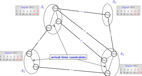
(27) Chapter 1. Background. 12. x15 x4 x5. x12 x1. x2 x8. x14. x16 x3. x10. x9. x13 x6. x7 x11. (a) The 16 provinces of Morocco.. (b) The map-coloring problem represented as a constraint graph.. Figure 1.3 – An example of the graph-coloring problem.. meetings among various people with respect to their personal calendars. The meeting scheduling problem has been defined in many versions with different parameters (e.g, duration of meetings [Wallace and Freuder, 2002], preferences of agents [Sen and Durfee, 1995], etc). In MSP, we have a set of attendees, each with his/her own calendar (divided on time-slots), and a set of n meetings to coordinate. In general, people/participants may have several slots reserved for already filled planning in their calendars. Each meeting mi takes place in a specified location denoted by location(mi ). The proposed solution must enable the participating agents to travel among locations where their meetings will be hold. Thus, an arrival-time constraint is required between two meetings mi and m j when at least one attendee participates on both meetings. The arrival time constraint between two meetings mi and m j is defined in Equation 1.1:. | time(mi ) − time(m j ) | −duration > TravelingTime(location(mi ), location(m j )).. (1.1). The meeting scheduling problem [Meisels and Lavee, 2004] can be encoded in a centralized constraint satisfaction problem as follows: • X = {m1 , . . . , mn } is the set of variables, each variable represents a meeting. • D = { D (m1 ), . . . , D (mn )} is a set of domains where D (mi ) is the domain of variable/meeting (mi ). D (mi ) is the intersection of time-slots from the personal calendar \ of all agents attending mi (i.e., D (mi ) = calendar ( A j )). A j ∈ attendees of mi. • C is a set of arrival-time constraints. There exists an arrival-time constraint for every pair of meetings (mi , m j ) if there is an agent that participates in both meetings. A simple instance of a meeting scheduling problem is illustrated in Figure 1.4. There.

(28) 1.2. Algorithms and Techniques for Solving Centralized CSPs. Med August 2011 1 8. 13. Adam August 2011. m14. meeting 4. 2 3 4 5 6 7 9 10 11 12 13 14. 6=. 1 8. m44. 2 3 4 5 6 7 9 10 11 12 13 14. m13. m11. meeting 4 meeting 1. August 2011 1 8. meeting 4. meeting 3. m21. 2 3 4 5 6 7 9 10 11 12 13 14. m34. 6=. m33. 6=. m22. meeting 2. Alice. Fred. m32. August 2011 1 8. 2 3 4 5 6 7 9 10 11 12 13 14. Figure 1.4 – A simple instance of the meeting scheduling problem.. are 4 attendees: Adam, Alice, Fred and Med, each having its personal calendar. There are 4 meetings to be scheduled. The first meeting (m1 ) will be attended by Alice and Med. Alice and Fred will participate on the second meeting (m2 ). The agents going to attend the third meeting (m3 ) are Fred and Med while the last meeting (m4 ) will be attended by three persons: Adam, Fred and Med. The instance presented in Figure 1.4 is encoded as a centralized CSP in Figure 1.5. The nodes are the meetings/variables (m1 , m2 , m3 , m4 ). The edges represent binary arrivaltime constraint. Each edge is labeled by the person, attending both meetings. Thus, • X = { m1 , m2 , m3 , m4 }. • D = { D (m1 ), D (m2 ), D (m3 ), D (m4 )}. – D (m1 ) = {s | s is a slot in calendar ( Alice) ∩ calendar ( Med)}. – D (m2 ) = {s | s is a slot in calendar ( Alice) ∩ calendar ( Fred)}. – D (m3 ) = {s | s is a slot in calendar ( Adam) ∩ calendar ( Fred) ∩ calendar ( Med)}. – D (m4 ) = {s | s is a slot in calendar ( Adam) ∩ calendar ( Fred) ∩ calendar ( Med)}. • C = {c12 , c13 , c14 , c23 , c24 , c34 }, where cij is an arrival-time constraint between mi and m j . These examples show the power of the CSP paradigm to easily model different combinatorial problems arising from different issues. In the following section, we describe the main generic methods for solving a constraint satisfaction problem.. 1.2 Algorithms and Techniques for Solving Centralized CSPs In this section, we describe the basic methods for solving constraint satisfaction problems. These methods can be considered under two board approaches: constraint propagation and search. We also describe here a combination of those two approaches. In general,.

(29) Chapter 1. Background. 14. m1. m2. Alice Med. Med attends meetings: m1 , m2 and m4 Alice attends meetings: m1 and m2. Fred. Fred Fred attends meetings: m2 , m3 and m4. Med. Adam attends meetings: m4 m4. Med, Fred, Adam. m3. Figure 1.5 – The constraint graph of the meeting-scheduling problem.. the search algorithms explore all possible combinations of values for the variables in order to find a solution of the problem, that is, a combination of values for the variables that satisfies the constraints. However, the constraint propagation techniques are used to reduce the space of combinations that will be explored by the search process. Afterwards, we present the main heuristics used to boost the search in the centralized CSPs. We particularly summarize the main variable ordering heuristics while we briefly describe the main value ordering heuristics used in the constraint satisfaction problems.. 1.2.1. Algorithms for solving centralized CSPs. Usually, algorithms for solving centralized CSPs search systematically through the possible assignments of values to variables in order to find a combination of these assignments that satisfies the constraints of the problem. An assignment of value vi to a variable xi is a pair ( xi , vi ) where vi is a value from the domain of xi (i.e., vi ∈ D ( xi )). We often denote this assignment by xi = vi .. Definition 1.5. Henceforth, when a variable is assigned a value from its domain, we say that the variable is assigned or instantiated. An instantiation I of a subset of variables { xi , . . . , xk } ⊆ X is an ordered set of assignments I = {[( xi = vi ), . . . , ( xk = vk )] | v j ∈ D ( x j )}. The variables assigned on an instantiation I = [( xi = vi ), . . . , ( xk = vk )] are denoted by vars(I) = { xi , . . . , xk }.. Definition 1.6. A full instantiation is an instantiation I that instantiates all the variables of the problem (i.e., vars(I) = X ) and conversely we say that an instantiation is a partial instantiation if it instantiates in only a part. Definition 1.7. An instantiation I satisfies a constraint cij ∈ C if and only if the variables involved in cij (i.e., xi and x j ) are assigned in I (i.e., ( xi = vi ), ( x j = v j ) ∈ I) and the pair (vi , v j ) is allowed by cij . Formally, I satisfies cij iff ( xi = vi ) ∈ I ∧ ( x j = v j ) ∈ I ∧ (vi , v j ) ∈ cij .. Definition 1.8. Definition 1.9. An instantiation I is locally consistent iff it satisfies all of the constraints whose.

(30) 1.2. Algorithms and Techniques for Solving Centralized CSPs. scopes have no uninstantiated variables in I. I is also called a partial solution. Formally, I is locally consistent iff ∀cij ∈ C | scope(cij ) ⊆ vars(I), I satisfies cij . Definition 1.10. A solution to a constraint network is a full instantiation I, which is locally. consistent. The intuitive way to search a solution for a constraint satisfaction problem is to generate and test all possible combinations of the variable assignments to see if it satisfies all the constraints. The first combination satisfying all the constraints is then a solution. This is the principle of the generate & test algorithm. In other words, a full instantiation is generated and then tested if it is locally consistent. In the generate & test algorithm, the consistency of an instantiation is not checked until it is full. This method drastically increases the number of combinations that will be generated. (The number of full instantiation considered by this algorithm is the size of the Cartesian product of all the variable domains). Intuitively, one can check the local consistency of instantiation as soon as its respective variables are instantiated. In fact, this is systematic search strategy of the chronological backtracking algorithm. We present the chronological backtracking in the following. 1.2.1.1. Chronological Backtracking (BT). The chronological backtracking [Davis et al., 1962; Golomb and Baumert, 1965; Bitner and Reingold, 1975] is the basic systematic search algorithm for solving CSPs. The Backtracking (BT) is a recursive search procedure that incrementally attempts to extend a current partial solution (a locally consistent instantiation) by assigning values to variables not yet assigned, toward a full instantiation. However, when all values of a variable are inconsistent with previously assigned variables (a dead-end occurs) BT backtracks to the variable immediately instantiated in order to try another alternative value for it. When no value is possible for a variable, a dead-end state occurs. We usually say that the domain of the variable is wiped out (DWO). Definition 1.11. Algorithm 1.1: The chronological Backtracking algorithm. procedure Backtracking(I) 01. if ( isFull(I) ) then return I as solution; /* all variables are assigned in I */ 02. else 03. select xi in X \ vars(I) ; /* let xi be an unassigned variable */ 04. foreach ( vi ∈ D ( xi ) ) do 05. xi ← vi ; 06. if ( isLocallyConsistent(I ∪ {( xi = vi )}) ) then 07. Backtracking(I ∪ {( xi = vi )});. The pseudo-code of the Backtracking (BT) algorithm is illustrated in Algorithm 1.1. The BT assigns a value to each variable in turn. When assigning a value vi to a variable xi , the consistency of the new assignment with values assigned thus far is checked (line 6, Algorithm 1.1). If the new assignment is consistent with previous assignments BT attempts to extend these assignments by selecting another unassigned variable (line 7). Otherwise (the. 15.

(31) Chapter 1. Background. 16. new assignment violates any of the constraints), another alternative value is tested for xi if it is possible. If all values of a variable are inconsistent with previously assigned variables (a dead-end occurs), backtracking to the variable immediately preceding the dead-end variable takes place in order to check alternative values for this variable. By the way, either a solution is found when the last variable has been successfully assigned or BT can conclude that no solution exist if all values of the first variable are removed. On the one hand, it is clear that we need only linear space to perform the backtracking. However, it requires time exponential in the number of variables for most nontrivial problems. On the other hand, the backtracking is clearly better than “generate & test” since a subtree from the search space is pruned whenever a partial instantiation violates a constraint. Thus, backtracking can detect early unfruitful instantiation compared to “generate & test”. Although the backtracking improves the “generate & test”, it still suffer from many drawbacks. The main one is the thrashing problem. Thrashing is the fact that the same failure due to the same reason can be rediscovered an exponential number of times when solving the problem. Therefore, a variety of refinements of BT have been developed in order to improve it. These improvements can be classified under two main schemes: lookback methods as conflict directed backjumping or look-ahead methods such as forward checking. 1.2.1.2 Conflict-directed Backjumping (CBJ) From the earliest works in the area of constraint programming, researchers were concerned by the trashing problem of the Backtracking, and then proposed a number of tools to avoid it. backjumping concept was one of the pioneer tools used for this reason. Thus, several non-chronological backtracking (intelligent backtracking) search algorithms have been designed to solve centralized CSPs. In the standard form of backtracking, each time a dead-end occurs the algorithm attempts to change the value of the most recently instantiated variable. However, backtracking chronologically to the most recently instantiated variable may not address the reason for the failure. This is no longer the case in the backjumping algorithms that identify and then jump directly to the responsible of the dead-end (cul prit). Hence, the culprit variable is re-assigned if it is possible or an other jump is performed. By the way, the subtree of the search space where the thrashing may occur is pruned. Given a total ordering on variables O , a constraint cij is earlier than ckl if the latest variable in scope(cij ) precedes the latest one in scope(ckl ) on O . Definition 1.12. Given the lexicographic ordering on variables ([ x1 , . . . , xn ]), the constraint c25 is earlier than constraint c35 because x2 precedes x3 since x5 belongs to both scopes (i.e., scope(c25 ) and scope(c35 )). Example 1.1. Gaschnig designed the first explicit non-chronological (backjumping) algorithm (BJ) in [Gaschnig, 1978]. BJ records for each variable xi the deepest variable with which it checks.

(32) 1.2. Algorithms and Techniques for Solving Centralized CSPs. its consistency with the assignment of xi . When a dead-end occurs on a domain of a variable xi , BJ jumps back to the deepest variable, say x j , to witch the consistency of xi is checked against. However, if there are no more values remaining for x j , BJ perform a simple backtrack to the last assigned variable before assigning x j . Dechter presented in [Dechter, 1990; Dechter and Frost, 2002] the Graph-based BackJumping (GBJ) algorithm, a generalization of the BJ algorithm. Basically, GBJ attempts to jump back directly to the source of the failure by using only information extracted from the constraint graph. Whenever a dead-end occurs on a domain of the current variable xi , GBJ jumps back to the most recent assigned variable (x j ) adjacent to xi in the constraint graph. Unlike BJ, if a dead-end occurs again on a domain of x j , GBJ jumps back to the most recent variable xk connected to xi or x j . Prosser proposed the Conflict-directed BackJumping (CBJ) that rectify the bad behavior of Gaschnig’s algorithm in [Prosser, 1993]. Algorithm 1.2: The Conflict-Directed Backjumping algorithm. procedure CBJ(I) 01. if ( isFull(I) ) then return I as solution; /* all variables are assigned in I */ 02. else 03. choose xi in X \ vars(I) ; /* let xi be an unassigned variable */ 04. EMCS[i ] ← ∅ ; 05. D ( xi ) ← D 0 ( xi ) ; 06. foreach ( vi ∈ D ( xi ) ) do 07. xi ← vi ; 08. if ( isConsistent(I ∪ ( xi = vi )) ) then 09. CS ← CBJ(I ∪ {( xi = vi )}) ; 10. if ( xi ∈ / CS ) then return CS ; 11. else EMCS[i ] ← EMCS[i ] ∪ CS \ { xi } ; 12. else 13. remove vi from D ( xi ) ; 14. let cij be the earliest violated constraint by (xi = vi ); 15. EMCS[i ] ← EMCS[i ] ∪ x j ; 16. return EMCS[i ] ;. The pseudo-code of CBJ is illustrated in Algorithm 1.2. Instead of recording only the (deepest variable, CBJ records for each variable xi the set of variables that were in conflict with some assignment of xi . Thus, CBJ maintains a set of earliest minimal conflict set for each variable xi (i.e., EMCS[i ]) where it stores the variables belonging to the earliest violated constraints with an assignment of xi . Whenever a variable xi is chosen to be instantiated (line 3), CBJ initializes EMCS[i ] to the empty set. Next, CBJ initializes the current domain of xi to its initial domain (line 5). Afterward, a consistent value vi with the current search state is looked for variable xi . If vi is inconsistent with the current partial solution, then vi is removed from current domain D ( xi ) (line 13), and x j such that cij is the earliest violated constraint by the new assignment of xi (i.e., xi = vi ) is then added to the earliest minimal conflict set of xi , i.e., EMCS[i ] (line 15). EMCS[i ] can be seen as the subset of the past variables in conflict with xi . When a dead-end occurs on the domain of a variable xi , CBJ jumps back to the last variable, say x j , in EMCS[i ] (lines 16,9 and line 10). The information in EMCS[i ] is earned upwards to EMCS[ j] (line 11). Hence, CBJ performs a form of “in-. 17.

(33) Chapter 1. Background. 18. telligent backtracking” to the source of the conflict allowing the search procedure to avoid rediscovering the same failure due to the same reason. When a dead-end occurs, the CBJ algorithm jumps back to address the culprit variable. During the backjumping process CBJ erases all assignments that were obtained since and then wastes a meaningful effort done to achieve these assignments. To overcome this drawback Ginsberg (1993) have proposed Dynamic Backtracking. 1.2.1.3 Dynamic Backtracking (DBT) In the naive chronological of backtracking (BT), each time a dead-end occurs the algorithm attempts to change the value of the most recently instantiated variable. Intelligent backtracking algorithms were developed to avoid the trashing problem caused by the BT. Although, these algorithms identify and then jump directly to the responsible of the deadend (cul prit), they erase a great deal of the work performed thus far on the variables that are backjumped over. When backjumping, all variables between the culprit of the dead-end and the variable where the dead-end occurs will be re-assigned. Ginsberg (1993) proposed the Dynamic Backtracking algorithm (DBT) in order to keep the progress performed before the backjumping. In DBT, the assignments of non conflicting variables are preserved during the backjumping process. Thus, the assignments of all variables following the culprit are kept and the culprit variable is moved to be the last among the assigned variables. In order to detect the culprit of the dead-end, CBJ associates a conflict set (EMCS[i ]) to each variable (xi ). EMCS[i ] contains the set of the assigned variables whose assignments are in conflict with a value from the domain of xi . In a similar way, DBT uses nogoods to justify the value elimination [Ginsberg, 1993]. Based on the constraints of the problem, a search procedure can infer inconsistent sets of assignments called nogoods. A nogood is a conjunction of individual assignments, which has been found inconsistent, either because the initial constraints or because searching all possible combinations. Definition 1.13. The following nogood ¬[( xi = vi ) ∧ ( x j = v j ) ∧ . . . ∧ ( xk = vk )] means that assignments it contains are not simultaneously allowed because they cause an inconsistency. Example 1.2. A directed nogood ruling out value vk from the initial domain of variable xk is a clause of the form xi = vi ∧ x j = v j ∧ . . . → xk 6= vk , meaning that the assignment xk = vk is inconsistent with the assignments xi = vi , x j = v j , . . .. When a nogood (ng) is represented as an implication, the left hand side, lhs(ng), and the right hand side, rhs(ng), are defined from the position of →. Definition 1.14. In DBT, when a value is found to be inconsistent with previously assigned values, a directed nogood is stored as a justification of its removal. Hence, the current domain D ( xi ) of a variable xi contains all values from its initial domain that are not ruled out by a stored nogood. When all values of a variable xi are ruled out by some nogoods, a dead-end occurs, DBT resolves these nogoods producing a new nogood (newNogood). Let x j be the most recent variable in the left-hand side of all these nogoods and x j = v j , that is x j is the culprit variable in the CBJ algorithm. The lhs(newNogood) is the conjunction of the.

(34) 1.2. Algorithms and Techniques for Solving Centralized CSPs. left-hand sides of all nogoods except x j = v j and rhs(newNogood) is x j 6= v j . Unlike the CBJ, DBT only removes the current assignment of x j and keeps assignments of all variables between it an xi since they are consistent with former assignments. Therefore, the work done when assigning these variables is preserved. The culprit variable x j is then placed after xi and a new assignment for it is searched since the generated nogood (newNogood) eliminates its current value (v j ). Since the number of nogoods that can be generated increases monotonically, recording all of the nogoods as is done in Dependency Directed Backtracking algorithm [Stallman and Sussman, 1977] requires an exponential space complexity. In order to keep a polynomial space complexity, DBT stores only nogoods compatible with the current state of the search. Thus, when backtracking to x j , DBT destroys all nogoods containing x j = v j . As a result, with this approach a variable assignment can be ruled out by at most one nogood. Since each nogood requires O(n) space and there are at most nd nogoods, where n is the number of variables and d is the maximum domain size, the overall space complexity of DBT is in O(n2 d). 1.2.1.4. Partial Order Dynamic Backtracking (PODB). Instead of backtracking to the most recently assigned variable in the nogood, Ginsberg and McAllester proposed the Partial Order Dynamic Backtracking (PODB), an algorithm that offers more freedom than DBT in the selection of the variable to put on the right-hand side of the directed nogood [Ginsberg and McAllester, 1994]. thereby, PODB is a polynomial space algorithm that attempted to address the rigidity of dynamic backtracking. When resolving the nogoods that lead to a dead-end, DBT always select the most among the set of inconsistent assignments recent assigned variable to be the right hand side of the generated directed nogood. However, there are clearly many different ways of representing a given nogood as an implication (directed nogood). For example, ¬[( xi = vi ) ∧ ( x j = v j ) ∧ · · · ∧ ( xk = vk )] is logically equivalent to [( x j = v j ) ∧ · · · ∧ ( xk = vk )] → ( xi 6= vi ) meaning that the assignment xi = vi is inconsistent with the assignments x j = v j , . . . , xk = vk . Each directed nogood imposes ordering constraints, called the set of safety conditions for completeness [Ginsberg and McAllester, 1994]. Since all variables in the left hand side of a directed nogood participate in eliminating the value on its right hand side, these variable must precede the variable on the right hand side. safety conditions imposed by a directed nogood (ng) ruling out a value from the domain of x j are the set of assertions of the form xk ≺ x j where xk is a variable in the left hand side of ng (i.e., xk ∈ vars(lhs(ng))). Definition 1.15. The Partial Order Dynamic Backtracking attempts to offer more freedom in the selection of the variable to put on the right-hand side of the generated directed nogood. In PODB, the only restriction to respect is that the partial order induced by the resulting directed nogood must safety the existing partial order required by the set of safety conditions, say S. In a later study, Bliek shows that PODB is not a generalization of DBT and then proposes the Generalized Partial Order Dynamic Backtracking (GPODB), a new algorithm that generalizes. 19.

(35) Chapter 1. Background. 20. both PODB and DBT [Bliek, 1998]. To achieve this, GPODB follows the same mechanism of PODB. The difference between two resides in the obtained set of safety conditions S0 after generating a new directed nogood (newNogood). The new order has to respect the safety conditions existing in S0 . While S and S0 are the similar for PODB, when computing S0 GPODB relaxes from S all safety conditions of the form rhs(newNogood) ≺ xk . However, both algorithms generates only directed nogoods that satisfy the already existing safety conditions in S. In the best of our knowledge, no systematic evaluation of either PODB or GPODB have been reported. All algorithms presented previously incorporates a form of look-back scheme. Avoiding possible future conflicts may be more attractive than recovering from them. In the backtracking, backjumping and dynamic backtracking, we can not detect that an instantiation is unfruitful till all variables of the conflicting constraint are assigned. Intuitively, each time a new assignment is added to the current partial solution, one can look ahead by performing a forward check of consistency of the current partial solution. 1.2.1.5 Forward Checking (FC) The forward checking (FC) algorithm [Haralick and Elliott, 1979; Haralick and Elliott, 1980] is the simplest procedure of checking every new instantiation against the future (as yet uninstantiated) variables. The purpose of the forward checking is to propagate information from assigned to unassigned variables. Then, it is classified among those procedures performing a look-ahead. Algorithm 1.3: The forward checking algorithm. procedure ForwardChecking(I) 01. if ( isFull(I) ) then return I as solution; /* all variables are assigned in I */ 02. else 03. select xi in X \ vars(I) ; /* let xi be an unassigned variable */ 04. foreach ( vi ∈ D ( xi ) ) do 05. xi ← vi ; 06. if ( Check-Forward(I, ( xi = vi )) ) then 07. ForwardChecking(I ∪ {( xi = vi )}); 08. else 09. foreach ( x j ∈ / vars(I) such that ∃ cij ∈ C ) do restore D ( x j ); function Check-Forward(I, xi = vi ) 10. foreach ( x j ∈ / vars(I) such that ∃ cij ∈ C ) do 11. foreach ( v j ∈ D ( x j ) such that (vi , v j ) ∈ / cij ) do remove v j from D ( x j ) ; 12. if ( D ( x j ) = ∅ ) then return false; 13. return true;. The pseudo-code of FC procedure is presented in Algorithm 1.3. FC is a recursive procedure that attempts to foresee the effects of choosing an assignment on the not yet assigned variables. Each time a variable is assigned, FC checks forward the effects of this assignment on the future variables domains (Check-Forward call, line 6). So, all values from the domains of future variables which are inconsistent with the assigned value (vi ) of the current variable (xi ) are removed (line 11). Future variables concerned by this filtering.