CIRPÉE
Centre interuniversitaire sur le risque, les politiques économiques et l’emploi
Cahier de recherche/Working Paper 06-05
Heterogeneous Basket Options Pricing Using Analytical
Approximations
Georges Dionne
Geneviève Gauthier
Nadia Ouertani
Nabil Tahani
Février/February 2006
_______________________
Dionne: Canada Research Chair in Risk Management, HEC Montréal and CIRPÉE Gauthier: Management Science Department, HEC Montréal
Ouertani: IESEG School of Management, Lille
Tahani: School of Administrative Studies, York University
The authors acknowledge the financial support of the Institut de Finance Mathématiques de Montréal (IFM2), the National Science and Engineering Research Council of Canada (NSERC) and the Fonds Québécois de Recherche sur la Société et la Culture (FQRSC). This paper extends N. Ouertani’s Ph.D. thesis on which Phelim P. Boyle, Michel Denault, and Pascal François have made very helpful suggestions. We also thank Moshe A. Milevsky and Chris Robinson for their comments. Previous versions of this paper have been presented at the 18th Annual Australasian Finance and Banking Conference (Sydney, December 2005) and the Northern Finance Association Meeting (Vancouver, October 2005).
Abstract: This paper proposes the use of analytical approximations to price an
heterogeneous basket option combining commodity prices, foreign currencies and
zero-coupon bonds. We examine the performance of three moment matching
approximations: inverse gamma, Edgeworth expansion around the lognormal and
Johnson family distributions. Since there is no closed-form formula for basket
options, we carry out Monte Carlo simulations to generate the benchmark values. We
perform a simulation experiment on a whole set of options based on a random choice
of parameters. Our results show that the lognormal and Johnson distributions give
the most accurate results.
Keywords: Basket Options, Options Pricing, Analytical Approximations, Monte Carlo
Simulation
JEL Classification: C15, C16, G10, G13
Résumé: Cet article traite de la tarification des options paniers hétérogènes en
présence de taux d’intérêt stochastiques. Nous proposons d’utiliser les
approximations analytiques pour tarifer une option panier hétérogène qui combine à
la fois des denrées, des taux de change et des obligations zéro-coupon. Nous avons
comparé la performance de trois approximations basées sur la technique
d’appariement des moments : la distribution gamma inverse, l’expansion Edgeworth
autour de la distribution lognormale et la famille de distributions de Johnson. Puisqu’il
n’existe pas de solution analytique au prix de l’option panier, nous avons utilisé les
simulations de Monte Carlo pour générer les valeurs de référence. Deux
expériences de simulation ont été menées, l’une basée sur une analyse de
sensibilité locale et l’autre, plus générale, basée sur un choix aléatoire de
paramètres. Nos résultats montrent que les approximations lognormale et Johnson
sont très précises et beaucoup plus performantes que l’approximation gamma
inverse.
Mots clés: Options panier, tarification d’option, approximation analytique, simulation
1
Introduction
The use of derivative securities in risk management activities emerged in the early 1990s and has evolved rapidly since. They now are the most important tool in …nancial risk management. Accord-ing to the 1998 Wharton school survey of …nancial risk management by US non-…nancial …rms,1
over 50% of the responding …rms use derivatives products to hedge their exposure, 83% of them use derivatives to hedge foreign-exchange risk, 76% to hedge interest-rate risk, and 56% to hedge commodity-price risk. In the current economic situation, many non-…nancial institutions such as gold-mining …rms, energy companies or airlines companies may face di¤erent …nancial risks simul-taneously and hence look for the most e¢ cient way to hedge their portfolio.
For example, gold-mining …rms may be exposed to di¤erent types of risk: commodity risk, which can include uncertainty about the price of their primary product, gold, as well as their by-products such as silver and copper; since these …rms sell their products in other countries, they are exposed to currency risk; and their interest rate risk exposure is primarily related to their …xed-rate and variable-rate debt. Though all these markets are very active and very liquid so that a …rm could hedge all its di¤erent risk exposures separately, it would be more interesting to adopt a portfolio approach because it allows the …rm to account for the correlations between these di¤erent …nancial markets and hedge simultaneously a great variety of di¤erent …nancial risks. To attain this goal, basket options are an e¢ cient instrument to use.
Basket options are a type of exotic option whose payo¤ depends on the value of a basket of assets. They o¤er the ‡exibility of being able to include virtually any kind and any number of assets, and hence can suitably respond to the speci…c needs of a …rm in hedging its risk exposures. A risk manager may have other incentives in using basket options: depending on the design of each option, they are usually cheaper than a portfolio of standard options. In practice, basket options are traded over-the-counter and are designed speci…cally to meet the needs of the buyer. For these reasons, the liquidity premium required by the counterpart may annihilate some of the advantages coming from the correlation structure of the basket.
The pricing of basket options is more challenging than that of standard options because there is no explicit analytical solution for the density function of a weighted sum of correlated assets. Several approaches are proposed in the literature to price basket options. They can be categorized as follows:
1. Numerical methods: Monte Carlo simulations [Barraquand (1995), Pellizzari (2001)] and Quasi-Monte Carlo [Dahl (2000) and Dahl and Benth (2001)], and multinomial trees [Ru-binstein (1994), Wan(2002)],
2. Upper and lower bounds: Curran (1994), Vanmaele, Deelstra and Liinev (2004), Laurence and Wang (2004) and Deelstra, Liinev and Vanmaele (2004),
3. Analytical approximations: Gentle (1993), Huynh (1994), Milevsky and Posner (1998a, 1998b, 1999), Posner and Milevsky (1999), Ju (2002), Datey, Gauthier and Simonato (2003) and Brigo, Mercurio, Rapisarda and Scotti (2004).
1
However, all these papers are based on two main hypothesis. They assume constant interest rates and homogeneous basket options; that is, all the assets underlying the basket are of the same nature and thus hedge the same type of risk. Unfortunately, this homogeneity in basket assets does not always match a …rm’s needs, and with a growing diversi…cation in investors’portfolios, heterogeneous basket options become a very e¢ cient tool to hedge multiple risk exposures simultaneously.
This article proposes analytical approximations to price heterogeneous basket options, consist-ing of commodities, foreign currencies and zero-coupon bonds, with stochastic interest rates, and compares the accuracy and the performance of these approximations for di¤erent sets of paramet-ers. Three distributions based on the moment matching technique will be used to approximate the basket density function: inverse gamma distribution, Edgeworth expansion around the lognormal distribution and Johnson distribution. It is found that the Edgeworth-lognormal and Johnson ap-proximations perform better than the inverse gamma approximation. Our contributions are: (1) to design an arbitrage-free framework in which the domestic and the foreign interest rates, the exchange rate, the commodity price and the convenience yield are stochastic, (2) to compute the moments of the heterogeneous basket under the T forward measure, (3) to show that some of the existing analytical approximations may be used in this very general setting and (4) quantify the approximation errors.
The next section presents the pricing model under the forward measure. Section 3 derives the inverse gamma, the Edgeworth-lognormal and the Johnson approximations. Section 4 compares the performance of the three approximations. Section 5 computes the hedging ratios and Section 6 concludes.
2
Pricing of a European heterogeneous basket option
Let us consider a non-…nancial …rm looking for an alternative way to simultaneously hedge its di¤erent …nancial risk exposures: commodity price risk, exchange rate risk and interest rate risk. In the following, St denotes the time t value of the commodity, t is its continuously-compounded
convenience yield at time t, Ct is the value at time t of one unit of the foreign currency expressed
in the domestic currency, P (t; T1) is the time t value of a zero-coupon bond paying one unit of the
domestic currency at time T1, P (t; T2) is the time t value of a foreign zero-coupon bond paying
one unit of the foreign currency at time T2. We assume that the …rm’s …nancial assets dynamics
are given by the following stochastic di¤erential equations2 (SDE hereafter) under the historical
2
In this setting, the convenience yield and the commodity price share the same source of risk to ensure the market completeness. For more details, see Dionne, Gauthier and Ouertani (2006).
probability measure P : dSt= St h ( s t) dt + sdWt(1) i ; (1a) d t= ( t)dt + dWt(1); (1b) dCt= Ct h cdt + cdWt(2) i ; (1c) dP (t; T1) = P (t; T1) rt t;T1 t;T1 t;T1 t;T1 dt t;T1dW (3) t ; 0 t T1; (1d) dP (t; T2) = P (t; T2) " rt t;T2 t;T2 t;T2 t;T2 !! dt t;T2dWt(4) # ; 0 t T2 (1e)
The expressions for the bond prices are obtained from the domestic and the foreign instantaneous forward rates: df (t; T1) = t;T1 dt + t;T1 dW (3) t ; 0 t T1; (1f) df (t; T2) = t;T2 dt + t;T2 dW (4) t ; 0 t T2; (1g)
in which the volatility parameters t;T1 and t;T
2are deterministic functions of time t and maturity.
Consequently, t;T1 =RT1
t t;sds, t;T2 =
RT2
t t;sds and rt = f (t; t) ; rt = f (t; t) are respectively
the continuously-compounded domestic and foreign risk-free spot interest rates. We do not specify the drift terms t;T1 and t;T
2 since they do not appear in the pricing formulae. The four-dimensional
Brownian motion Wt(1); Wt(2); Wt(3); Wt(4) 0 : t 0 is constructed on a …ltered probability space ( ; F; fFt: t 0g ; P ) with the correlation structure:
CorrP Wt(i); Wt(j) = i;j; for each i; j = f1; 2; 3; 4g and t > 0:
We consider an European call option that gives the …rm the right to buy a basket consisting of the commodity, the domestic zero-coupon bond and the foreign zero-coupon bond expressed in domestic currency units, at a strike price KB. The payo¤ at maturity T is given by
XB = max [BT KB; 0] ;
where the basket value at time t is Bt = w1St+ w2P (t; T1) + w3CtP (t; T2), 0 t T T1; T2,
w1; w2 and w3 correspond to the numbers of shares invested respectively in the commodity ST,
the domestic zero-coupon bond P (T; T1) and the foreign zero-coupon bond expressed in domestic
currency units CTP (T; T2).
Since the proposed market model is complete,3 Harrison and Pliska (1981) allows the pricing of any contingent claim as the expectation of the discounted payo¤ under the risk-neutral measure Q. Consequently, the price of the European call option at time t is given by:
VtB = EQ exp Z T t rvdv max (BT KB; 0) Ft = P (t; T )EQT[ max (B T KB; 0)j Ft] = P (t; T ) Z +1 1 max (x KB; 0) v (x) dx; (2)
where v (x) is the true (unknown) density function of the basket value BT under the T forward
measure QT. This forward measure has a Radon-Nikodym derivative with respect to Q denoted dQT
dQ : The associated Q martingale is given by:
t= EQ
dQT
dQ Ft =
exp RtTrvdv
P (t; T ) :
The SDEs satis…ed by the basket underlying assets under the T -forward measure QT is given in
Appendix A and its strong solution is, for any 0 t T , ST = Stexp Z T t ru u 2 s 2 s 1;3 u;T du + s Z T t dcWu(1) (3a) T = te (T t)+ s s 1 e (T t) 1;3 Z T t e (T u) u;T du + s Z T t rue (T u) du + Z T t e (T u) dcWu(1) (3b) CT = Ctexp Z T t ru ru 2 c 2 c 2;3 u;T du + c Z T t dcWu(2) (3c) P (T; T1) = P (t; T1) exp Z T t ru 1 2 2
u;T1 + u;T1 u;T du
Z T t u;T1 dcWu(3) (3d) P (T; T2) = P (t; T2) exp RT t ru 12 u;T2 2
+ c 2;4 u;T2 + 3;4 u;T2 u;T du
RT t u;T2dcW (4) u ! (3e)
where cW = Wc(1); cW(2); cW(3); cW(4) 0 is a QT Brownian motions with CorrQT Wct(i); cW (j)
t =
i;j.
The evaluation of the basket call option is complicated by the absence of a closed-form equation for the density function v(x) in Equation (2). Among the di¤erent approaches proposed in the basket options literature, we …nd some numerical techniques such as Monte Carlo, Quasi-Monte Carlo and lattice-based methods, the upper and lower bound computations,4 and some analytical approximations.
Lattice-based approaches are widely used for options on a single asset. They are, exponentially complicated and computationally expensive for options on multiple assets. For example, our three-asset basket option needs (n + 1)3 terminal nodes on an n-step trinomial tree. On the other hand, Monte Carlo and Quasi-Monte Carlo methods can be used for multi-assets options and are less time-consuming than lattice-based approaches. The estimates can be as accurate as needed at a computational cost however: to improve the accuracy of an n-path simulation by one half, one needs to simulate 4n paths and thus needs 4 times more computing time.
A practitioner might be interested in slightly less accurate but very fast methods such as ana-lytical approximations. These methods approximate the unknown basket density function with an alternative and easy-to-compute distribution. In the next sections, we will extend three well-known
4The upper and lower bounds methods are not useful in our case since the market model proposed is complete and
analytical approximations to heterogeneous basket options: the inverse gamma distribution, the Edgeworth expansion around the lognormal distribution and Johnson distribution.
3
Analytical approximations
In order to apply these moment matching-based approximations, we need to calculate the …rst four moments of the weighted sum underlying the European option under the T forward measure QT.
We adopt the following notations:
0 n(h) = Z +1 1 xnh (x) dx (4a) n(h) = Z +1 1 x 01(h) nh (x) dx; (4b) 0
n(h) and n(h) represent respectively the nth non-centered and centered moments of the density
function h 2 fv; ag ; where h = v corresponds to the exact density of the basket value under the forward measure while h = a corresponds to the approximate density. The …rst four cumulants of distribution h, that is, the mean, the variance, the skewness and the kurtosis are de…ned as:
1(h) = 01(h) (5a)
2(h) = 2(h) (5b)
3(h) = 3(h) (5c)
4(h) = 4(h) 3 2(h) : (5d)
Lemma 1 For any positive integer n, the nth non-centered moment of the true distribution of the weighted sum BT; under the T -forward measure QT, is
0 n(v) = EQT [BnT] = EQT[(w1ST + w2P (T; T1) + w3CTP (T; T2))n] = n X k=0 k X j=0 n! j! (k j)! (n k)!w j 1w (k j) 2 w (n k) 3 EQT h STj (P (T; T1))(k j)CTn k(P (T; T2))n k i :
Note that the log normal distribution of ST, P (T; T1), CT, and P (T; T2) under the forward measure
allows the computation of the last expectation of Lemma 1 from following identity: E [exp ( + Z)] = exp +
2
2 where Z N (0; 1) : Details are given in Appendix B.
3.1 Inverse gamma approximation
In this section, we use the inverse gamma distribution to approximate the sum of correlated lognor-mal variables. This approximation was …rst used by Milevsky and Posner (1998a, 1998b) to price Asian and basket options. In fact, a …nite sum of correlated lognormal variables converges asymp-totically to an inverse gamma variable. Under an inverse gamma distribution for the underlying
basket, an European basket call option has a closed-form solution that looks like a Black and Scholes (1973) (B&S hereafter) formula:
VgammaB = P (t; T ) 01(v) G 1 KB 1; KBG 1 KB ; ; (6)
where G ( j ; ) is the cumulative function of a gamma distribution with parameters ( ; ). These parameters are determined by matching the …rst two moments of the exact and the approximate distributions to obtain: = 02 1 (v) 2 02(v) 02 1 (v) 02(v) and = 0 2(v) 021 (v) 0 1(v) 02(v) : (7)
Mathematical details of the pricing formula are provided in Appendix C. 3.2 Edgeworth expansion around the lognormal distribution
We now present an analytical approximation based on a generalized Edgeworth expansion around the lognormal distribution. This approach, introduced by Jarrow and Rudd (1982) in option pricing, substitutes an unknown density function v ( ) with a Taylor-like expansion around an easy-to-use density function denoted a ( ). Notice, however, that Edgeworth expansions usually lead to a function which is not a true density function. Barton and Denis (1952) derive some conditions on the third and fourth moments of the unknown distribution to guarantee that the approximation obtained with a truncated Edgeworth expansion is positive and unimodal. Moreover, Ju (2002) points out that the Edgeworth expansion may diverge for some parameter values, which consequently can give incorrect prices for high volatility and long maturity options. However, in this paper we do not have this problem in the application of the Edgeworth expansion.
Following Huynh (1994) who uses this approach for basket options, we will use an Edgeworth expansion of order 4 and we will match the …rst and second moments of the exact and the lognormal distributions. Under this approximation, an European basket call option can be obtained as a sort of Black and Scholes price adjusted for the excess skewness and the excess kurtosis from the lognormal density:
Vlog normalB = P (t; T ) V 3(v) 3(a)
3! da (KB) dx + 4(v) 4(a) 4! d2a (K B) dx2 ; (8a) where V = 01(v) N (d1) KBN (d2) ; (8b) d1 = d2+ ; (8c) d2 = ln (KB) ; (8d) = ln 01(v) 2 1 2ln 0 1(v) 2 + 2(v) ; (8e) = r ln 1 + 2(v) ( 01(v)) 2 ; (8f) a ( ) is the density function of a log-normal distribution (see Equation (19) in Appendix D), and N ( ) represents the cumulative function of the standard normal distribution. The third and fourth
moments of the lognormal distribution needed for the Edgeworth expansion depend only on the …rst and second moments of the exact distribution and are given by:
0 3(a) = 0 2(v) 0 1(v) 3 and 04(a) = 0 2(v) 6 0 1(v) 8: (8g)
Details about the Edgeworth approximation formula are given in Appendix D. 3.3 Johnson approximation
Johnson (1949) proposes a family of density functions, obtained via a transformation of a standard normal variable, that can be used to approximate unknown distributions. Let Z be a standard normal variable and X be a random variable with an unknown density function, Johnson (1949) suggests the following transformations between Z and X:
Z = + X " ; (9a)
X = " + 1 Z ; (9b)
where and are the shape parameters of the Johnson distribution, is the scale parameter, " is the threshold parameter, and ( ) is one of the following Johnson functions:
L(x) = ln (x) ; (Lognormal system) U(x) = ln x + p x2+ 1 ; (Unbounded system) B(x) = ln x 1 x . (Bounded system) The choice of the system and …tting parameters provides a great ‡exibility in adjusting the curve to match the …rst four moments of the unknown distribution. We use the lognormal ( L) and the unbounded ( U) systems that are common in the literature. We apply the Hill, Hill and Holder (1976) algorithm, based on the true skewness and kurtosis of the basket distribution, to determine which of the Johnson systems ( L or U) should be used in the approximation. Unlike approximations obtained with a truncated Edgeworth expansion, approximations based on Johnson (1949) systems correspond to true density functions with a perfect match of the …rst four moments. Following Posner and Milevsky (1999), we substitute the unknown distribution of the underlying basket with the lognormal and the unbounded Johnson functions where the system parameters are calculated by matching the four moments. Under a Johnson density function, a European basket call option can be priced as:
VJ ohnsonB = P (t; T ) Z +1 KB (x KB) (x) dx = P (t; T ) Z +1 0 x (x) dx KB Z +1 0 (x) dx Z KB 0 (x KB) (x) dx = P (t; T ) 01(v) KB+ Z KB 0 Z x 0 (y) dy dx = P (t; T ) 01(v) KB+ Z KB 1 Z x 0 (y) dy dx : (11)
The third line in the equation is obtained using an integration by parts. Milevsky and Posner (1999) show that the last double integral, involving a Johnson density function, can be computed as follows:
1. Lognormal system L: X = " + exp Z Z KB 1 Z x 0 (y) dy dx = (KB ") N + ln KB " exp 1 2 2 2 N + ln KB " 1 : (12)
2. Unbounded system U : X = " + sinh Z Z KB 1 Z x 0 (y) dy dx = (KB ") N (q) + 2 exp 1 2 2 exp N q + 1 2exp 1 2 2 exp N q 1 ; (13) where q = + sinh 1 KB " :5
4
Performance analysis of approximations
In this section, we analyze the performance of the three approximations presented previously. We will use prices obtained by Monte Carlo simulations as benchmarks since there is no closed-form solution for basket options. Following Barraquand (1995), we will apply a variance reduction tech-nique based on the matching of the …rst and second moments. This will ensure that sample mean and variance are equal to the their theoretical counterparts. The Monte Carlo basket option price combined with the variance reduction technique is given by:
VB0 = 1 N N X i=1 P (0; T ) max Bi;T KB; 0
where Bi;T = Bi;T B
p
2(v) bS 1+ 01(v) ;
Bi;T is the time T basket value obtained with sample path i; and B = m1 Pmi=1Bi;T and bS =
q 1 m Pm i=1Bi;T2 B 2
are respectively the sample basket mean and standard deviation and m is the number of simulated paths.
Our performance study will be conducted with two analyses. In the …rst sensitivity analysis, we will compare the basket option price obtained with the analytical approximations to the Monte Carlo price obtained with 1,000,000 paths repeated for di¤erent maturities, di¤erent moneynesses and di¤erent levels for the basket volatility. The second sensitivity analysis is a more detailed analysis based on works done by Broadie and Detemple (1996). It computes the option prices over a wide range of parameters chosen randomly from a realistic set of values in order to generalise our
5Notice that sinh (x) = exp(x) exp( x)
2 and thus sinh
1(x) = ln x +px2+ 1 = U(x):
previous results independently of the model’s parameters. For each combination, we compare the prices obtained with the approximations and Monte Carlo simulations.
Table 1 presents the set of parameters used in the …rst analysis. These values are based on estimations using real data on gold prices, CAD/USD exchange rate and Canadian and American 3-month zero-coupon bonds. Although we have positive and negative correlations in the set of parameters, the volatility of the basket will increase when individual assets volatilities increase.
Table 1: Parameters used in the …rst sensitivity analysis
Domestic risk-free rate,f (0; t) = f for any t 0.06
Foreign risk-free rate,f (0; t) = f for any t 0.05
Commodity drift, s 0.15
Exchange rate drift, c 0.04
Commodity volatility, s 0.15
Exchange rate volatility, c 0.06
Domestic instantaneous forward rate volatility, t;T1 = for any tandT1 0.01 Foreign instantaneous forward rate volatility, t;T
2 = for any tandT2 0.01
Convenience yield volatility, 0.3
Convenience yield mean reversion parameter, 0.1
Convenience yield long-run mean, 0.15
Commodity and exchange rate correlation, 1;2 0.1
Commodity and domestic instantaneous forward rate correlation, 1;3 -0.2 Commodity and foreign instantaneous forward rate correlation, 1;4 -0.25 Exchange rate and domestic instantaneous forward rate correlation, 2;3 0.05 Exchange rate and foreign instantaneous forward rate correlation, 2;4 0.1 Foreign and domestic instantaneous forward rates correlation, 3;4 0.85
Basket weights (commodity, domestic and foreign zero-coupon bonds) 0.5; 0.25; 0.25
Initial pricesS0; C0 and 0 are respectively $330; $/CAD 0.65; 0.2
Table 2 presents sensitivity analysis of the basket option price with respect to moneyness, which corresponds to the ratio of the exercise price over the initial value of the basket KB
B0; and option
maturity. The results show that Edgeworth-lognormal and Johnson approximations are much more accurate, with relative errors between 10 6 and 10 3, than the inverse gamma approximation with a relative error between 10 4 and 10 1.6
6This result is consistent with Milevsky and Posner (1998a) who showed that the convergence result for the inverse
gamma works well when the risk-neutral drift of the underlying di¤usion is negative or when the correlation matrix decays quickly.
Table 2: Sensitivity analysis w.r.t. the moneyness and option maturity
Moneyness Monte Standard Inverse Gamma Lognormal Johnson Carlo Deviation Approximation Approximation Approximation
Price Relative Price Relative Price Relative
error error error
0.75-year maturity
0.85 14.6677 9.16e-03 14.6496* 1.23e-03 14.6678 4.60e-06 14.6676 5.06e-06
0.95 3.1876 5.33e-03 3.1890 4.50e-04 3.1879 7.94e-05 3.1879 8.57e-05
1 0.9173 2.84e-03 0.9400* 2.47e-02 0.9175 2.87e-04 0.9177 4.75e-04
1.05 0.1842 1.21e-03 0.2008* 9.02e-02 0.1843 7.06e-04 0.1844 1.36e-03
1.15 0.0026 1.28e-04 0.0039* 4.69e-01 0.0026 4.91e-03 0.0027 7.76e-03
1-year maturity
0.85 15.1267 1.12e-02 15.0876* 2.59e-03 15.1266 1.02e-05 15.1263 3.07e-05
0.95 4.3557 7.08e-03 4.3517 9.09e-04 4.3557 1.80e-05 4.3557 1.65e-05
1 1.7612 4.54e-03 1.7915* 1.72e-02 1.7616 2.26e-04 1.7619 3.67e-04
1.05 0.5828 2.54e-03 0.6180* 6.06e-02 0.5830 3.82e-04 0.5833 8.51e-04
1.15 0.0359 5.79e-04 0.0460* 2.81e-01 0.0360 1.97e-03 0.0361 3.89e-03
1.5-year maturity
0.85 22.8033 2.19e-02 22.6061* 8.65e-03 22.8037 1.70e-05 22.8022 4.84e-05
0.95 12.597 1.77e-02 12.465* 1.05e-02 12.5976 4.47e-05 12.5967 2.19e-05
1 8.8786 1.52e-02 8.8241* 6.14e-03 8.8792 6.63e-05 8.8790 4.15e-05
1.05 6.0473 1.28e-02 6.0704 3.81e-03 6.0470 5.47e-05 6.0474 6.31e-06
1.15 2.5478 8.33e-03 2.6693* 4.77e-02 2.5475 1.11e-04 2.5485 2.91e-04
3-year maturity
0.85 110.1708 1.35e-01 106.8891* 2.98e-02 110.182 1.02e-04 110.1632 6.92e-05
0.95 99.7516 1.33e-01 95.7420* 4.02e-02 99.7590 7.41e-05 99.7385 1.32e-04
1 94.8429 1.31e-01 90.5429* 4.53e-02 94.8574 1.53e-04 94.8363 6.91e-05
1.05 90.1511 1.30e-01 85.5986* 5.05e-02 90.1621 1.22e-04 90.1408 1.14e-04
1.15 81.3707 1.26e-01 76.4686* 6.02e-02 81.3813 1.30e-04 81.3601 1.30e-04
The Monte Carlo benchmarks are based on 106trajectories using moment matching as a variance reduction technique. The estimated standard deviations of the Monte Carlo prices are reported. The parameters used for the simulation are provided in Table 1. The maturity dates of the domestic and foreign bonds are respectivelyT1 = T + 90=360andT2= T + 120=360:Relative errors are computed ase = VB(a) VB =VB;where VB(a) andVB are the option prices obtained respectively with the analytical approximation and the Monte Carlo simulation. The prices marked with a star (*) are signi…cantly di¤erent from their Monte Carlo benchmark at a level of 5%.
Table 3 presents sensitivity analysis of the basket option price with respect to the basket volatility and option maturity, for in the money options, KB
B0 = 0:95. The average level volatility corresponds
to the values in Table 1, while high and low levels correspond respectively to an increase and a decrease of 50% in the volatility values given in Table 1.
Table 3: Sensitivity analysis with respect to the basket volatility and option maturity
Basket Monte Standard Inverse Gamma Lognormal Johnson Volatility Carlo Deviation Approximation Approximation Approximation
Price Relative Price Relative Price Relative
error error error
0.75-year maturity
Low 1.6122 2.63e-03 1.6132 5.76e-04 1.6124 7.90e-05 1.6124 8.36e-05
Average 3.1880 5.33e-03 3.1890 3.32e-04 3.1879 3.93e-05 3.1879 3.29e-05
High 4.5412 7.93e-03 4.5419 1.54e-04 4.5411 6.36e-06 4.5412 3.16e-06
1-year maturity
Low 2.3602 3.59e-03 2.3594 3.62e-04 2.3602 1.59e-05 2.3602 1.72e-05
Average 4.3556 7.08e-03 4.3517 8.93e-04 4.3557 3.44e-05 4.3557 3.29e-05
High 6.0694 1.05e-02 6.0578 1.92e-03 6.0697 4.43e-05 6.0697 4.25e-05
1.5-year maturity
Low 8.2211 9.43e-03 8.1845* 4.45e-03 8.2214 3.72e-05 8.2211 4.92e-06
Average 12.5963 1.77e-02 12.4650* 1.04e-02 12.5976 9.87e-05 12.5967 3.20e-05
High 16.9935 2.66e-02 16.6624* 1.95e-02 16.9940 2.67e-05 16.9921 8.69e-05
3-year maturity
Low 70.0721 5.75e-02 69.5164* 7.93e-03 70.0736 2.17e-05 70.0701 2.73e-05
Average 99.7475 1.33e-01 95.7420* 4.02e-02 99.7590 1.16e-04 99.7385 9.03e-05
High 149.5893 2.71e-01 138.7165* 7.27e-02 141.3625* 5.50e-02 149.5287 4.05e-04
The Monte Carlo benchmarks are based on 106trajectories using moment matching as a variance reduction technique. The estimated standard deviations of the Monte Carlo prices are reported. The parameters used for the simulation are provided in Table 1. The maturity dates of the domestic and foreign bonds are respectively T1 = T + 90=360andT2= T + 120=360 and the moneyness isKB=B0= 0:95Relative errors are computed ase = VB(a) V
B
=VB; where
VB(a) and VB are the option prices obtained respectively with the analytical approximation and the Monte Carlo simulation. The prices marked with a star (*) are signi…cantly di¤erent from their Monte Carlo benchmark at a level of 5%.
The …ndings are similar to those in Table 2. The relative errors presented in Table 3 are very low with a magnitude between 10 6 and 10 2. For low volatility levels, Edgeworth-lognormal and Johnson approximate prices and Monte Carlo prices are very close. As for the inverse gamma approximation, our results show that it is much less accurate with relative errors between 10 4 and 10 2.
volatilities, which supports the …ndings in Ju (2002).7 Moreover, for all approximations, option prices increase with maturity and volatility.
The previous analysis is only local. Our …ndings depend on the set of parameters used and may change if we modify them. To con…rm our conclusions, a more carefully designed numerical study where the parameters are randomly chosen is conducted. Following Broadie and Detemple (1996), the signi…cant model parameters are chosen randomly from continuous or discrete uniform distributions. These uniform distributions are based on the estimation of the model parameters using real data. The correlation between the commodity and the exchange rate is expected to be positive, so we assume that 12 2 [0:01; 0:55] : Based on Schwartz (1997), the convenience yield long-run mean is positive for gold and the mean reversion parameter is small and less than 1; we assume thus that 2 [0:05; 0:5] and 2 [0:05; 0:8]. All paramater distributions used in the pricing are presented in Table 4.
Table 4: Parameters distributions
Domestic risk free rate,f (0; t) = f for anyt U(0.02; 0.08)
Foreign risk free rate,f (0; t) = f for anyt U(0.02, 0.08)
Commodity drift, s U(0.05, 0.35)
Exchange rate drift, c 0.04
Commodity volatility, s U(0.1, 0.35)
Exchange rate volatility, c U(0.02, 0.15)
Domestic instantaneous forward rate volatility, t;T1 = for anyt andT1 U(0.001, 0.06) Foreign instantaneous forward rate volatility, t;T
2 = for anyt andT2 U(0.001, 0.06)
Convenience yield volatility, U(0.1, 0.4)
Convenience yield mean reversion parameter, U(0.05, 0.8)
Convenience yield long-run mean, U(0.05, 0.5)
Commodity and exchange rate correlation, 1;2 U(0.01, 0.55)
Commodity and domestic instantaneous forward rate correlation, 1;3 U( 0.5, 0.25) Commodity and foreign instantaneous forward rate correlation, 1;4 U( 0.5, 0.25) Exchange rate and domestic instantaneous forward rate correlation, 2;3 U( 0.35, 0.35) Exchange rate and foreign instantaneous forward rate correlation, 2;4 U( 0.35, 0.35) Foreign and domestic instantaneous forward rates correlation, 3;4 U(0.15, 0.9)
Option maturity (in years) U{0.083; 0.25; 0.5; 0.75; 1; 1.5; 2; 3}
Moneyness U{0.8; 0.9; 0.95; 1; 1.05; 1.1; 1.2}
Basket weights (commodity domestic and foreign zero-coupon bonds), U 13 13 13;12 14 41;14 12 14;14 14 12
Initial pricesS0; C0 and 0 are respectively $330; $/CAD 0.65; 0.2
We compare the three previous analytical approximations and Monte Carlo simulation combined with the moment matching technique for 5000 random sets of parameters. Only 4740 sets of parameters provided positive de…nite correlation matrices. We also removed all basket options
7Ju (2002) proposes an analytical approximation to price Asian and basket options based on a Taylor expansion of
the ratio of the characteristic function of the average of lognormal variables to that of the approximating lognormal random variable around zero volatility.
prices with a value lower than 5 cents. We obtained 4347 sets of parameters. First, we examine the accuracy of each approximation by calculating its root mean square error (RMSE). Second, we calculate the maximum relative error (MRE) for each approximation to examine the worst case scenario. More precisely, we de…ne,
RM SE = v u u t 1 n n X i=1 VB i (a) V B i VBi !2 M RE = max i ViB(a) VBi VBi ;
where n is the number of di¤erent sets of paramaters, that is, Monte Carlo prices are obtained with 1; 000; 000 paths combined with the moment matching technique.
Table 5: RMSE and MRE for the three approximations Inverse Gamma Lognormal Johnson
Approximation Approximation Approximation
RMSE 9.68% 0.52% 0.56%
MRE 79.47% 13.16% 14.00%
The results in Table 5 con…rm those obtained with the …rst sensitivity analysis (Tables 2 and 3) and show that the Edgeworth-lognormal and Johnson approximations are much more accurate than the inverse gamma approximation. It is also found that, for the Edgeworth-lognormal and Johnson approximations, a very small proportion of options, 0:23% and 0:35% respectively, have relative errors above 5% while for the inverse gamma approximation, a larger proportion, 27:74%, of options have a relative error above 5%.
A more detailed look at the results shows that out-of-the-money and high volatility options have the largest relative errors, which con…rms our …ndings in the …rst sensitivity analysis. However, since the out-of-the-money options have small prices, the augmentation of the relative errors in these cases may be attributed to the small denominators. Figures 1, 2 and 3 present respectively the histograms of the relative errors of the inverse gamma, the Edgeworth-lognormal and Johnson approximations. Table 6 shows a summary of descriptive statistics of the relative errors.
Figure 1: Histogram of relative errors of the inverse gamma approximation 0 0.1 0.2 0.3 0.4 0.5 0.6 0.7 0.8 0 500 1000 1500 2000 2500 3000
3500 Relative Errors Histogram for the Inverse Gamma Distribution
Relative Errors Number of Ob s ervat ions
X-axisrepresents relative errors
Figure 2: Histogram of relative errors of the Edgeworth approximation 0 0.02 0.04 0.06 0.08 0.1 0.12 0.14 0 500 1000 1500 2000 2500 3000 3500 4000
4500 Relative Errors Histogram for the Edgeworth-Lognormal Distribution
Relative Errors Nu mber of Ob s er v ations
X-axisrepresents relative errors
Y-axisrepresents the number of observations
Figure 3: Histogram of relative errors of Johnson approximation
-0.020 0 0.02 0.04 0.06 0.08 0.1 0.12 0.14 0.16 500 1000 1500 2000 2500 3000 3500 4000
4500 Relative Errors Histogram for the Johnson Distribution
Relative Errors N umbe r o f Obser v ations
X-axisrepresents relative errors
Table 6: Descriptive statistics of relative errors
Inverse Gamma Lognormal Johnson Approximation Approximation Approximation
Maximum 0.7947 0.1316 0.1400 Minimum 0 0 0 Mean 0.0493 0.0015 0.0014 Median 0.0136 0.0002 0.0001 Standard Deviation 0.0833 0.0050 0.0054 Nb of observations 4347 4347 4347
The histograms show that for the Edgeworth-lognormal and Johnson approximations, 99% of parameters sets (4300 out of 4347) have relative errors less than 2%: This demonstrates that these approximations are very accurate and that they give prices very close to Monte Carlo benchmarks. The inverse gamma approximation has 92% (4000 out of 4347) cases where the relative errors are less than 20%. We reach the same results by using larger and more general intervals for the parameters distributions.
To conclude this section regarding the pricing of heteregeneous basket options, we show that Edgeworth expansion around the lognormal distribution at order 4 and the Johnson distribution are equally accurate and very acceptable for practitionners. However, we suggest the use of the Edgeworth-lognormal distribution for two reasons: …rst, it is slightly more accurate, and second, the algorithm to calibrate Johnson distributions may not converge in a few cases, which can lead to mispriced options.
5
Hedging ratios
The analytical approximations allow for deriving the option price in a functional form which can also provide analytical expressions for the sensitivities with respect to the underlying parameters, such as deltas, vegas and theta, known as the hedging ratios or the Greeks. However, due to the complexity of the moments involved in our analytical approximations, deriving the hedging ratios analytically is beyond the scope of this article. Instead, we can compute them numerically as follows:
RatioBApp= V B(") App V B App " ; (14)
where " > 0 is a small number, VAppB(") and VAppB are respectively the approximate "-disturbed and non-disturbed option prices. As an application, we compute numerically the delta with respect to the commodity price for di¤erent values of ". We base our calculations on the parameters in Table 1. We consider an in-the-money call basket option KB
B0 = 0:95 with a 9-month maturity. The
Table 7: Basket option Delta w.r.t. the commodity price Commodity Inverse Gamma Lognormal Johnson
Price Approximation Approximation Approximation
Price Delta* Price Delta* Price Delta*
$330 3.1890 3.1879 3.1879
$330.33 3.1922 0.0097 3.1910 0.0094 3.1911 0.0097 $331.65 3.2049 0.0096 3.2037 0.0096 3.2038 0.0096 $333.30 3.2208 0.0096 3.2196 0.0096 3.2196 0.0096 $334.95 3.2367 0.0096 3.2355 0.0096 3.2355 0.0096
* Delta corresponds to the sensitivity with respect to the commodity price and is given by Equation (14). VB
App,presented in the …rst row of the table,is the analytical basket option price obtained for a commodity price of$330:
Table 7 shows that, for the three approximations, the delta is very stable over di¤erent values of ". Indeed, an increase of $1 in the commodity price leads to an increase of approximately $0:01 in the option price. The positiveness of delta is expected but its value depends on the set of parameters used. Following the same procedure, one can compute the other sensitivities with respect to other parameters of interest.
6
Conclusion
Firms can use basket options to hedge their exposure to di¤erent risks, such as commodity risk, interest rate risk and exchange rate risk. However, pricing this kind of options is not an easy task since no closed-form solution can be derived for the basket density function. Consequently, a standard pricing formula such as Black and Scholes cannot be derived. The main contribution of this article is the comparison of the performance of three analytical approximations to price a heteregeneous basket option, consisting of a commodity, a domestic and a foreign zero-coupon bonds, when interest rates are stochastic. The three approximations used are the inverse gamma proposed in Milevsky and Posner (1998a, 1998b), the Edgeworth expansion around the lognormal distribution as well as Johnson distribution developped in Posner and Milevsky (1999).
In order to assess and compare the accuracy of the approximations, we use two analyses. The …rst one is a local sensitivity analysis where the parameters of the model are …xed arbitrarily. Our …ndings show that both the Edgeworth-lognormal and Jonhson approximations are very accurate while the inverse gamma approximation is much less accurate.
These results are con…rmed with the second analysis where 5000 sets of parameters are chosen randomly from di¤erent uniform distributions. It is also found that the pricing relative errors, computed with Monte Carlo benchmark prices, are small and of an acceptable magnitude for prac-titionners. The accuracy of all approximations deteriorates for out-of-the-money as well as for high volatility options.
This article considers only plain vanilla basket options. However, extending the approach fol-lowed here to more exotic basket options is a promising area for future research.
Appendices
A
Derivation of the forward measure
In this appendix, we will derive the model under the T forward measure. Let Ai be the ith row of the
matrix A; where A = [aij]i;j=f1;2;3;4g is the Cholesky decomposition of the correlation matrix of the
four-dimensional P Brownian motions W = W(1); W(2); W(3); W(4) 0; and eB corresponds to the vector of
independent Brownian motions under Q. The SDEs satis…ed by all underlying assets under Q can be written as:8 dSt = St h (rt t) dt + sA1d eBt i (15a) d t = ( s ( s rt) t)dt + A1d eBt (15b) dCt = Ct h (rt rt) dt + cA2d eBt i (15c) dP (t; T1) = P (t; T1) h rtdt t;T1A3d eBt i (15d) dP (t; T2) = P (t; T2) h rt + t;T2 c 2;4 dt t;T2 A4d eBt i (15e) The risk-neutral measure Q corresponds to a numeraire equal to the domestic bank account exp RtTrudu ;
while the T forward measure QT corresponds to a numeraire equal to the domestic zero-coupon bond with
maturity date T , P (t; T ). Using Girsanov theorem, we have that: d bBt= d eBt+ t;TA03dt;
where bBare independent Brownian motions under QT. The correlation structure is the same under Q and
QT; and the previous SDEs can be rewritten as:
dSt = St h rt t 13 s t;T dt + sdcWt(1) i (16a) d t = ( s ( s rt) t 13 t;T)dt + dcW (1) t (16b) dCt = Ct h rt rt 23 c t;T dt + cdcWt(2) i (16c) dP (t; T1) = P (t; T1) h rt+ t;T1 t;T dt t;T1dcW (3) t i (16d) dP (t; T2) = P (t; T2) h rt+ t;T2 c 2;4+ 3;4 t;T t;T2 dt t;T2 dcW (4) t i (16e) where cW = cW(1); cW(2); cW(3); cW(4) 0 = A bB: The strong solution exists and is given by the system of
equations (3).
B
Derivation of moments
This appendix gives the detailed calculation of the …rst four moments of the basket value at maturity T under the T forward measure QT. Using the strong solution of the model under the forward-measure QT,
one can write ST = S0exp S(T ) + 4 X i=1 Z T 0 S;i (t) dcWt(i) ! P (T; T1) = exp P(T ) + 4 X i=1 Z T 0 P;i (t) dcWt(i) ! CTP (T; T2) = C0exp CP (T ) + 4 X i=1 Z T 0 CP ;i (t) dcWt(i) ! ; where S(T ) = 2 6 6 6 6 4 RT 0 1 s 1 e (T u) f (0; u) du 01 1 e T s s + 2s 2 T + s s 1 1 e T 1 2 RT 0 2 u;Tdu + s RT 0 1 e (T u) Ru 0 v;u v;T v;u dv du + 1;3R0T u;T 1 e (T u) s du 3 7 7 7 7 5; P(T ) = Z T1 T f (0; u) du 1 2 Z T 0 u;T1 u;T 2 du; CP (T ) = Z T 0 f (0; u) du Z T2 0 f (0; u) du 1 2 Z T 0 2 u;T + u;T2 2 du 2 c 2 T c 2;3 Z T 0 u;T du + c 2;4 Z T 0 u;T2 du + 3;4 Z T 0 u;T2 u;T du; S;1(t) = s 1 e (T t) ; S;3(t) = t;T s Z T t 1 e (T v) t;v dv; P;3(t) = t;T t;T1; CP ;2(t) = c; CP ;3(t) = t;T; CP ;4(t) = t;T2; S;2(t) = S;4(t) = P;1(t) = P;2(t) = P;4(t) = CP ;1(t) = 0; Therefore, 0 n = n X k=0 k X j=0 n! j! (k j)! (n k)!w j 1w (k j) 2 w (n k) 3 E QT hSj T(P (T; T1))k jCTn k(P (T; T2))n k i with EQT hSj T(P (T; T1))k jCTn k(P (T; T2))n k i = S0jC0n k(P (0; T2))n kEQT " exp (T ) + 4 X i=1 Z T 0 i (t) dcWt(i) !# = S0jC0n k(P (0; T2))n kexp (T ) + 1 2 4 X i=1 4 X `=1 i;` Z T 0 i (t) `(t) dt ! where (T ) = j S(T ) + (k j) P(T ) + (n k) P (T ) i(t) = j S:i(t) + (k j) P:i(t) + (n k) P :i(t) , i 2 f1; 2; 3; 4g :
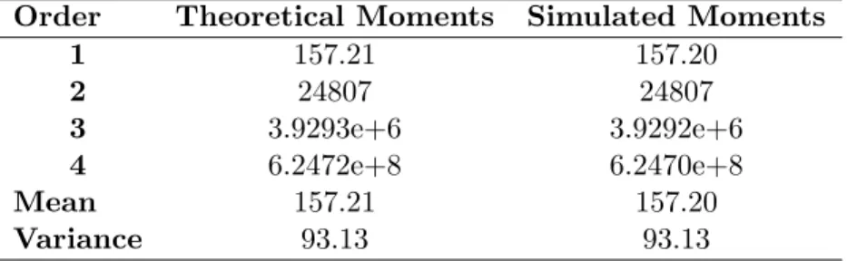
Table 8 presents the theoretical …rst four moments, calculated as explained previously, and those obtained by Monte Carlo simulation. This ensures that our theoretical formulas give the exact moments.
Table 8: Comparison of theoretical and simulated moments Order Theoretical Moments Simulated Moments
1 157.21 157.20 2 24807 24807 3 3.9293e+6 3.9292e+6 4 6.2472e+8 6.2470e+8 Mean 157.21 157.20 Variance 93.13 93.13
C
Inverse gamma approximation
This appendix shows how we obtain the pricing formula using the inverse gamma approximation. The density function of a gamma random variable X of parameters ( ; ) ; X s G ( ; ) ; is given by:
g (x j ; ) =
x 1exp x
( ) ; x 0
where > 0; > 0 and ( ) is the Gamma function.
Proposition 1Let X be a gamma random variable with parameters ( ; ) : Then, the random variable Y = X1; follows an inverse gamma distribution, Y s GR( ; ) ; and its density function is given by:
gR(y j ; ) = 1 y2g 1 yj ; = exp y1 y +1 ( ); y > 0; ; > 0: (17)
Proposition 2The non-centered moments of the random variable Y s GR( ; ) are given by: 0
n(gR) =
1
n( 1) ( 2) ::: ( n); n = 1; 2; 3; ::: (18)
We price the basket option by approximating the sum of lognormal variables by an inverse gamma distribution. We match the two …rst moments
0 1(v) = 01(gR) = 1 ( 1) and 0 2(v) = 02(gR) = 1 2( 1) ( 2);
the option price P (t; T )R+11max (x KB; 0) v (x) dx is approximated by: VgammaB = P (t; T ) Z +1 KB (x KB) gR( xj ; ) dx = P (t; T ) Z +1 KB (x KB) x 2g 1 x ; dx = P (t; T ) Z 1 KB 0 1
y KB g ( yj ; ) dy from the change of variable y = 1 x = P (t; T ) 1 ( 1) Z 1 KB 0 g ( yj 1; ) dy KB Z 1 KB 0 g ( yj ; ) dy ! since 1 yg ( yj ; ) = 1 ( 1)g ( yj 1; ) = P (t; T ) 1 ( 1) G 1 KB 1; KB G 1 KB ; leading to Equation (6).
D
Edgeworth-lognormal expansion
This appendix shows how we obtain the pricing formula using an Edgeworth expansion around the lognormal distribution. Matching the …rst two moments, the lognormal density used is given by
a (x) = p1 2 1 1 xexp 1 2 ln x 2! (19) where and are de…ned at lines (8e) and (8f) respectively. Following Jarrow and Rudd (1982), the unkown basket density function can be approximated by:
v (x) = a (x) + 2(v) 2(a) 2! d2a (x) dx2 3(v) 3(a) 3! d3a (K) dx3 +( 4(v) 4(a)) + 3 ( 2(v) 2(a)) 2 4! d4a (x) dx4 + (x) ; (20)
where (x) is an error term and i(h) ; i = f1; 2; 3; 4g are the …rst four cumulants of the density function
h = fv; ag de…ned by the system of Equations (5). Jarrow and Rudd (1982) state that, in general, there is no bound on the error term resulting from an Edgeworth expansion. Consequently, the error does not necessarily decrease with the expansion’s order. Given that the two …rst moments are the same for the true density and for the approximated density, Equation (20) becomes
v (x) = a (x) 3(v) 3(a) 3! d3a (K) dx3 + 4(v) 4(a) 4! d4a (x) dx4 + (x) : (21)
The basket option price P (t; T )R+1
1 max (x KB; 0) v (x) dx can thus be approximated by:
Vlog normalB = P (t; T ) Z +1 KB (x KB) a (x) 3 (v) 3(a) 3! d3a (x) dx3 + 4(v) 4(a) 4! d4a (x) dx4 dx:
Using the fact that
Z +1 KB (x KB) dja dxj (x) dx = dj 2a dxjB 2(KB) for j 2;
we obtain Vlog normalB = P (t; T ) Z +1 KB (x KB) a (x) dx 3 (v) 3(a) 3! da dx(KB) + 4(v) 4(a) 4! d2a dx2(KB) : (22)
Notice that the …rst integral in Equation (22) is very similar to a Black and Scholes price.
References
[1] Barraquand, J., 1995. "Numerical Valuation of High Dimensional Multivariate European Securities". Management Science, 41, 12, 1882-1891.
[2] Barton, D. E. and Dennis, K. E. R., 1952. "The Conditions Under Which Gram-Charlier and Edgeworth Curves are Positive de…nite and Unimodal," Biometrika, 39, 425-427
[3] Baxter, M. and Rennie, A., 1996. "Financial Calculus, An Introduction to Derivative Pricing". Cam-bridge, New York.
[4] Black, F. and Scholes, M., 1973. "The Pricing of Options and Corporate Liabilities". The Journal of Political Economy, 81, 3, 637-659.
[5] Brigo, D., Mercurio, F., Rapisarda, F. and Scotti, R., 2004. "Approximated Moment-Matching for Basket-options Pricing". Quantitative Finance, 4, 1-16.
[6] Broadie, M. and Detemple, J., 1996. "American Option Valuation: New Bounds, Approximations and a Comparison of Existing Methods". The Review of Financial Studies, 9, 4, 1211-1250.
[7] Carmona, R. and Durrleman, V., 2003. "Pricing and Hedging Multivariate Contingent Claims", Working paper, Princeton University.
[8] Castellacci, G. and Siclari, M.J., 2003. "Asian Basket Spreads and Other Exotic Averaging Options". Energy Power Risk Management.
[9] Curran, M., 1994. "Valuing Asian and Portfolio Options by Conditioning on the Geometric Mean Price". Management Science, 40, 12, 1705-1711.
[10] Dahl, L.O., 2000. "Valuation of European Call Options on Multiple Underlying Assets by Using a Quasi-Monte Carlo Method. A Case with Baskets from Oslo Stock Exchange". In Proceedings AFIR 2000, 10, 239-248.
[11] Dahl, L.O. and Benth, F.E., 2001. "Valuation of Asian Basket Options with Quasi-Monte Carlo Tech-niques and Singular Value Decomposition". Pure Mathematics, 5, 1-21.
[12] Datey, J.Y., Gauthier, G. and Simonato, J.G., 2003. "The Performance of Analytical Approximations for the Computation of Asian-Quanto-Basket Option Prices". The Multinational Finance Journal, 7, 1, 55-82.
[13] Deelstra, G., Liinev, J. and Vanmaele, M., 2004. "Pricing of Arithmetic Basket Options by Condition-ing". Insurance: Mathematics and Economics, 34, 1, 1-23.
[14] Dionne, G., Gauthier, G. and Ouertani, N., 2006. "Basket Options on Heterogeneous Underlying Assets". Working paper, HEC Montréal (forthcoming).
[15] Flamouris, D. and Giamouridis, D., 2004. "Valuing Exotic Derivatives with Jump Di¤usions: The Case of Basket Options". Working Paper, Athens University of Economics and Business.
[16] Gentle, D., 1993. "Basket Weaving". Risk, 6, 6, 51-52.
[17] Harrison, J.M. and Pliska, S.R., 1981. "Martingales and Stochastic Integrals in the Theory of Continuous Trading". The Stochastic Processes and Their Applications, 11, 261-271.
[18] Hill, I., Hill, R. and Holder, R., 1976. "Fitting Johnson Curves by Moments". Applied Statistics, 25, 2, 180-192.
[19] Huynh, C.B., 1994. "Back to Baskets". Risk, 5, 59-61.
[20] Jarrow, R. and Rudd, A., 1982. "Approximate Option Valuation for Arbitrary Stochastic Processes". Journal of Financial Economics, 10, 3, 347-369.
[21] Johnson, N.L., 1949. "Systems of Frequency Curves Generated by Methods of Translation". Biometrika, 36, 149-176.
[22] Ju, N., 2002. "Pricing Asian and Basket Options via Taylor Expansion". The Journal of Computational Finance, 5, 3, 79-103.
[23] Laurence, P. and Wang, T.H., 2004. "What’s a Basket Worth?". Risk, 17, 2, 73-77.
[24] Milevsky, M.A. and Posner, S.E., 1998a. "Asian Options, the Sum of Lognormals and the Reciprocal Gamma Distribution". The Journal of Financial and Quantitative Analysis, 33, 3, 409-422
[25] Milevsky, M.A. and Posner, S.E., 1998b. "A Closed-Form Approximation for Valuing Basket Options". The Journal of Derivatives, 5, 4, 54-61.
[26] Milevsky, M.A. and Posner, S.E., 1999. "Another Moment for the Average Option". Derivatives Quarterly, 47-53.
[27] Pellizzari, P., 2001. "E¢ cient Monte Carlo Pricing of European Options Using Mean Value Control Variates". Decisions in Economics and Finance, 24, 107-126
[28] Posner, S.E. and Milevsky, M.A., 1999. "Valuing Exotic Options by Approximating the SPD with Higher Moments". The Journal of Financial Engineering, 7, 2, 109-125.
[29] Rubinstein, M., 1994. "Return to Oz". Risk, 7, 67-71.
[30] Vanmaele, M., Deelstra, G. and Liinev, J., 2004. "Approximation of Stop-Loss Premiums Involving Sums of Lognormals by Conditioning on Two Variables". Insurance: Mathematics and Economics, 35, 343-367.
[31] Vyncke, D., Goovaerts, M. and Dhaene, J., 2003. "An Accurate Analytical Approximation for the Price of a European-Style Arithmetic Asian Option", Working paper, K.U. Leuven, Dept. of Applied Economics, Belgium
[32] Wan, H., 2002. "Pricing American-Style Basket Options by Implied Binomial Tree", Working paper, Haas School of Business, University of California at Berkeley