HAL Id: hal-00362877
https://hal.archives-ouvertes.fr/hal-00362877
Submitted on 19 Feb 2009
HAL is a multi-disciplinary open access
archive for the deposit and dissemination of
sci-entific research documents, whether they are
pub-lished or not. The documents may come from
teaching and research institutions in France or
abroad, or from public or private research centers.
L’archive ouverte pluridisciplinaire HAL, est
destinée au dépôt et à la diffusion de documents
scientifiques de niveau recherche, publiés ou non,
émanant des établissements d’enseignement et de
recherche français ou étrangers, des laboratoires
publics ou privés.
Supervision of an industrial plant subject to a maximal
duration constraint
Abdourrahmane Atto, Claude Martinez, Saïd Amari
To cite this version:
Abdourrahmane Atto, Claude Martinez, Saïd Amari. Supervision of an industrial plant subject to
a maximal duration constraint. 9th International Workshop on Discrete Event Systems, May 2008,
Göteborg, Sweden. pp.254-259. �hal-00362877�
Supervision of an industrial plant subject to a maximal duration
constraint
Abdourrahmane M. ATTO
Claude MARTINEZ
Sa¨ıd AMARI
Abstract— This paper presents a method for the supervision of an industrial plant. This supervision is aimed at guaranteeing the respect of a maximal duration constraint for some specific processing, and is addressed by considering a discrete event system model for this industrial plant. In this associated model, the time constraint is reduced to elementary constraints whose contributions are taken into account in the state equation of the system, yielding a constrained state equation for the plant. Supervisors are then synthesized by looking for solutions of this constrained state equation.
Keywords: Discrete event systems, (max, +) algebra, time constraints, supervisor, control.
I. INTRODUCTION
This work concerns the supervision of a manufacturing unit that produces rubber hoses for the automotive industry. The development of this industry requires optimization of its productivity, while respecting a strict temporal constraint for specific processing. The sizing of this industrial plant has been solved and validated via computational simulations in [1], and the resource optimization for the manufacturing unit has been treated in [2]. The problem addressed in this paper concerns the supervision of the plant in order to guarantee the respect of a strict temporal constraint for the thermal treat-ments involved. The supervision is aimed at guaranteeing that this time constraint is met without impacting significantly the production rate of the manufacturing unit. It is shown that this supervision can be performed thanks to analytical techniques.
The industrial plant studied can be modelled as a Discrete Event System (DES). Several approaches have been proposed for the analysis of DES these last few decades [3]. A DES can be modelled with a Timed Event Graph (TEG) [4], [5] when it represents phenomena requiring synchronisations and excluding competition as well as conflict. The analysis of such a system can then be described with linear equations in (max, +)-algebra [4], [6]. The industrial plant under consideration satisfies these assumptions. Thus, in order to guarantee the time constraint imposed, we propose solutions based on the constrained(max, +) state equation of the TEG model of the plant.
Performance evaluation is of great interest in the literature on the (max, +)-algebra topic [4], [6], [7]. In this appli-cation, the performance of a supervisor will be measured according to the maximum production throughput of the supervised plant. According to this particular performance
EMIG Niamey, [email protected]
IUT Nantes, [email protected] ENS Cachan, [email protected]
measure, we can classify supervisors between those which slow down the production throughput and those which pre-serve this production rate. The cycle time of such a plant modelled as a TEG corresponds to the eigenvalue of the matrix associated with its graph [6], [8], [9], the production throughput is the inverse of the cycle time. Similar problems of meeting time constraints have been recently addressed with different approaches[10], [11], [12], [13].
This work is organised as follows. Section II briefly recalls the fundamentals of (max, +) algebra, section III presents a TEG model for the plant and gives its corresponding linear(max, +) model. Section IV addresses the supervision problem and provides a simple way for synthesizing super-visors for time constrained systems. This section provides 3 supervisors for the manufacturing plant and classifies them by showing that some preserve the production throughput of the plant, in comparison to that of the non-supervised plant. Finally, section V gives a conclusion and addresses perspectives to extend this work.
II. (max, +)ALGEBRA
This section briefly recalls the fundamentals of(max, +) algebra, which is largely used for the analysis of DES. Further details on this theory may be found in [4], [6], [14], [15]. In what follows,D denotes a set.
Definition 1 (Monoid): A monoid is an algebraic set with an associative internal operation and an identity element.
Definition 2 (Semiring): (D, ⊕, ⊗) is a semiring if: • (D, ⊕) is a commutative monoid. Its identity element
is denoted by� (null element).
• (D, ⊗) is a monoid. Its identity element is denoted by e (unit element).
• Multiplication⊗ distributes over addition and every x ∈ D is such that x ⊗ � = � ⊗ x = �.
Definition 3 (Dioid): A dioid(D, ⊕, ⊗) is an idempotent semiring (everyx ∈ D is such that x ⊕ x = x).
Hereafter, the producta ⊗ b will be denoted a.b or ab when there is no possible confusion.
Example 1: Examples of dioids:
• Let R be the set of real numbers. (R ∪ {−∞}, max, +) is a commutative dioid for which� = −∞ and e = 0. This dioid is denoted by Rmax and is called(max, +) algebra.
• Let (D, ⊕, ⊗) be a dioid and Dn×n the set of square matrices of order n over D. (Dn×n, ⊕, ⊗) is a dioid called a matrix dioid. The sum and the matrix product are defined as follows: ifA = (Aij), B = (Bij), then (A ⊕ B)ij = Aij⊕ Bij and(A ⊗ B)ij=�nk=1Aik⊗
Proceedings of the 9th International Workshop on Discrete Event Systems Göteborg, Sweden, May 28-30, 2008
Bkj. The null element of the matrix dioid is the matrix composed of�. The unit matrix is the matrix with e on the main diagonal and � elsewhere.
III. TEGREPRESENTATION AND LINEAR(max, +) MODEL FOR A MANUFACTURING UNIT
A Petri net consists of places, directed arcs, and transi-tions. Directed arcs connect places and transitions (there is no direct connection between two places or between two transitions). TEGs are a subclass of Petri Nets in which every place is connected to only one input and one output transitions. According to the nature of the problem tackled in this paper, we focus on the particular case where crossing transitions is instantaneous. In such cases, temporisations are set only over places [5]. The temporisation associated with each place corresponds to the minimum duration of a specific process running in this place and marked by a token. Each transitionxjis associated with a function that gives the firing time for thekth occurrencex
j(k).
A nice example of TEG is that of the manufacturing unit of the industrial plant under consideration. This unit specialises in manufacturing rubber tubes for automotive equipment and is represented in figure 1. This figure represents three
con-1 2 3 A I O E
Fig. 1. Manufacturing unit.
veyor belts connected in loops. Loops 1 and 2 are identical. Each one is composed of a loading station (A, on loop 2) where parts subject to heat treatment are fixed on specific pallets, a unloading station (E) where parts are dismounted, and a furnace (IO cells). The furnace itself consists of two parts, a heating zone and a cooling zone. The parts are subjected to high temperatures during the time they spent in the first half of the furnace. Then, they are cooled in the second half. After cooling of parts, pallets are brought to the unloading station where an operator removes the parts from the pallets and dispatches them in batches towards another unit of the production workshop. The transport device is not always available for the evacuation of treated parts and this could cause an accumulation of pallets at the unloading station. In such cases, saturation may occur at the entry of the unloading station, causing the system to block. The pallets present in the furnace then exceed their processing time and the embarked products are burned and lost. Thus, for this application, the time spent in the heating zone is critical: the maximal heating time should not be exceeded even when
non-evacuation of treated products occurs at the unloading station.
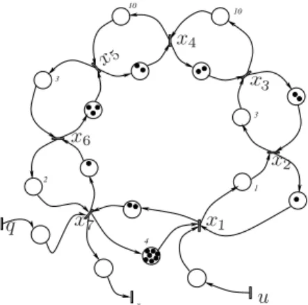
Loops 1 and 2 being identical, we can restrict our attention in one loop (2 in the sequel). We adopt an analytical approach to solve the supervision problem for this application. This manufacturing unit reveals synchronisations between loops. Indeed, loading pallet is possible only if an empty pallet and parts to supply it are present at the loading station A. In the same way, availability of the transport device is necessary at the unloading station to take away the treated parts (station E) and make available an empty pallet for forthcoming use. This type of industrial plant requiring synchronisations can be modelled as a TEG. The TEG model of this application is that of figure 2. In this graph, transitions are associated
y 4 1 3 10 10 3 2 u q x1 x2 x3 x4 x5 x6 x7
Fig. 2. TEG model for loop 2 of the industrial plant.
with the following events: • u: arrival of the parts;
• x1: beginning of the loading operation; • x2: starting transport to the furnace;
• x3: entry to the heating zone of the furnace; • x4: entry to the cooling zone of the furnace; • x5: starting transport to the evacuation zone; • x6: beginning of the unloading operation; • x7: part evacuation;
• q: transport device (may be present or absent). • y: departure of the parts.
The input transition u models the arrival of parts to be treated and the transitionq models the transport device for evacuating finished parts. When the transport device fails, saturation can occur because of non-evacuation of treated products. The output transition y corresponds to actually treated and evacuated parts. Crossing transition xi corre-sponds to the occurrence of an event, for example, crossing x1 corresponds to the beginning of the loading operation on a pallet, x2 to the end of this operation and the beginning of transport to the furnace. Operation durations are indicated close to places; for example, the transfer of a pallet from the loading station to the entry of the furnace (station I) is about 3 time units.
Tokens (in places) model the resources of the manufac-turing unit: pallets, operators, capacity of conveyors, etc. For instance, the transfer time from unloading station E
to loading station A is four time units. In addition, there are actually seven free pallets and there remain two places available on the conveyor (in the graph of figure 2).
The state vector,x, of this TEG is composed of transitions x1, x2, · · · , x7; and the input vector, v, is composed of transitions u and q. The state and output equations that describe the dynamic behaviour of the TEG of figure 2 are given in (max, +)-algebra by
x1(k + 1)= x2(k) ⊕4x7(k − 6) ⊕u(k + 1), x2(k + 1)=1 x1(k + 1)⊕ x3(k − 1), x3(k + 1)=3 x2(k + 1)⊕ x4(k − 1), x4(k + 1)=10x3(k + 1)⊕ x5(k − 1), x5(k + 1)=10x4(k + 1)⊕ x6(k − 2), x6(k + 1)=3 x5(k + 1)⊕ x7(k), x7(k + 1)=2 x6(k + 1)⊕ x1(k − 1) ⊕q(k + 1), y(k) = x7(k). (1)
In these equations, ⊕ denotes the max operator and the multiplication corresponds to the natural element addition in the set of real numbers (see [4], [6] for further details about (max, +)-algebra). These equations yield a matrix representation where statex(k) at time k depends on states x(k), x(k−1), x(k−2), x(k−3), x(k−7) and on input v(k). However, there exists a simplified representation of the TEG state of the form:x(k+1) = A0x(k+1)⊕Ax(k)⊕Bv(k+1). Indeed, a place with m tokens and temporisation α is equivalent tom places, each of them having only one token and temporisation αi, with � αi = α. According to this decomposition, the TEG model of the manufacturing unit is that of figure 3 (reduction from depth7 to depth 1).
y 1 3 10 10 3 2 4 u q x1 x2 x3 x4 x5 x6 x7 x8 x9 x10 x11 x12 x13 x14 x15 x16 x17 x18 x19
Fig. 3. Simplified model for loop 2 of the manufacturing unit.
The dynamic behaviour of the simplified TEG obtained (figure 3) is described by a system of the form:
�
x(k + 1) = H0x(k + 1) ⊕ H1x(k) ⊕ K0v(k + 1), y(k) = Sx(k),
(2) where matricesK0,H0,H1andS are omitted here because of their large size and the limited length of the present paper.
After reduction (using the Kleene star operator, see [6], [4]), system Eq. (2) is equivalent to:
�
x(k + 1) = Hx(k) ⊕ Kv(k + 1),
y(k) = Sx(k), (3) where H and K are given below. In these matrices, e = 0 denotes the unit element; and the null element, −∞, is replaced by a dot. H= 0 B B B B B B B B B B B B B B B B B B B B B B B B B B B B B @ . e . . . e . 1 . . . e . . . 1 . 4 . . . 3 e . . . 4 . 14 . . . 13 10 e . . . 14 . 24 . . . 23 20 10 e . . . 24 . 27 . . . . e 26 23 13 3 . . . 27 . 29 . . . . 2 28 25 15 5 . e . . . 29 . . e . . . . . . . e . . . . . . . . e . . . . . . . e . . . . . . . e . . . . e . . . . . . . 4 . . . . . . . e . . . . . . . . e . . . . . . . e . . . . . . e . . . . . e . 1 C C C C C C C C C C C C C C C C C C C C C C C C C C C C C A , and K= „ e 1 4 14 24 27 29 . . . . . . . e . . . . «t , wheret denotes matrix transposition.
IV. SUPERVISION OF THE INDUSTRIAL PLANT
A. Maximal duration constraints
The minimum duration of tokens in places is expressed by temporisations of these places. On the other hand, if we wish to express a maximum duration in a place, we must then add an additional constraint. Consider the TEG represented in figure 4. s xj xi xg τ (� τmax) β r
Fig. 4. Temporal constraint
Letpij be the place linking transition tj to transition ti, andpig the place linking transition tg to transition ti. The marking (number of tokens) of placepij isr. If we want to enforce a maximum time durationτmax to tokens in place pij, then the following inequality must be satisfied:
xi(k) � τmaxxj(k − r). (4) In addition, according to the graph of figure 4, transition ti firing is governed by:
wheres is the number of tokens in place pig, τ � τmax is the temporisation of placepij, andβ is the temporisation of placepig.
From Eqs. (4) and (5) we derive the (necessary and sufficient) condition under which a token will not exceed the duration constraintτmax in place pij:
βxg(k − s) � τmaxxj(k − r). (6) Note that for TEGs, a place with m > 1 tokens can be decomposed inm places with one token. For this reason, we focus on the special case where s − r = 1. The maximum duration constraint Eq. (4) is then expressed in the following form:
βxg(k − 1) � τmaxxj(k). (7) The next example shows how to express the maximum duration constraint in the form of Eq. (7).
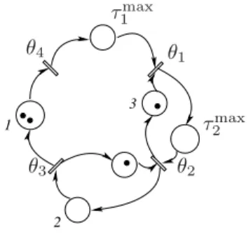
Example 2: Consider the TEG given in figure 5. Durationsτmax
1 andτ max
2 are the normal durations of tokens
3 1 2 θ1 θ2 θ3 θ4 τmax 1 τmax 2
Fig. 5. TEG with two duration constraints.
in corresponding places and these durations should not be exceeded. The constraints are:
(a) θ1(k) � τ max 1 θ4(k), and (b) θ2(k) � τ max 2 θ1(k). These constraints are respected if:
(a) true if 3θ2(k − 1) � τ max 1 θ4(k), (b) true if θ3(k − 1) � τ max 2 θ1(k), that is, if „ � � e � � 3 � � « θ(k) � „ τmax 2 � � � � � � τmax 1 « θ(k + 1), withθ = (θ1θ2θ3θ4) t .
Consider a TEG governed by a state equation of the form (general state representation)
�
x(k + 1) = Ax(k) ⊕ Bv(k + 1),
y(k) = Cx(k). (8) Assume that we want to impose on this TEG, a set of time constraints of the form
Ex(k) � F x(k + 1). (9) whereE and F are � × n matrices, � being the number of constraints andn the length of the state vector x.
Supervisors guaranteeing that the constraints Eq. (9) are met can be calculated by applying a state modification (constrained state equation) given by
x(k + 1) = (A ⊕ M )x(k) ⊕ Bv(k + 1), (10) whereM (supervision matrix) is a matrix satisfying
E � F M. (11) B. Constraint expression for the industrial plant
The supervision is aimed at preventing parts being lost because of possible failure in the transport device. The (max, +)-equation that governs the time spent by a part in the heating zone of the furnace is derived from the dynamic behaviour of the simplified TEG of figure 3 and is:
x4(k + 1) = 10x3(k + 1) ⊕ x10(k). (12) To avoid losing parts, a product should not exceed 10 time units in the heating zone of the furnace (place that links transitionx3 to transitionx4 in figures 2 and 3). Thus, the constraint will be respected by forcing
x4(k + 1) = 10x3(k + 1), (13) Taking Eq. (12) into account, condition Eq. (13) will be satisfied iff: x10(k) � 10x3(k + 1). (14) Denoting Q1= ` . . . e . . . ´ , Q2= ` . . 10 . . . ´ ,
the constraint condition Eq. (14) is thus of the form Eq. (9): Q1x(k) � Q2x(k + 1).
C. Supervision of the manufacturing unit
The dynamic behaviour of the manufacturing unit is de-scribed with the (max, +) system Eq. (3). The maximum duration constraint imposes Q1x(k) � Q2x(k + 1). A supervisor guaranteeing respect of the duration constraint can be calculated by searching for a matrixM0(supervision matrix) satisfying
Q1�Q2M0. (15) The only non null element ofQ1 being(Q1)1,10 = e, it is sufficient to consider the solutions of:
e � 19 � j=1 (Q2)1,j(M0)j,10, (16) that is, e � 10(M0)3,10. (17) The smallest positive (least restrictive) solution of the latter equation is (M0)3,10 = e. The supervision obtained from this solution involves adding to the graph of figure 3, a place having a single token (with no temporisation because (M0)3,10 = e ≡ 0) from transition x10 to transitionx3.
Let mx3 be the state of transition x3 after supervision. Firing of transitionmx3 is then subject to
mx3(k + 1) = x3(k + 1) ⊕ x10(k). (18)
Transition x10 being an auxiliary variable derived from the expansion of the original model of the manufacturing unit (represented by the graph of figure 2), we do not have access to this transition in practice: it is neither controllable, nor observable [16]. But from Eq. (3) we derive thatx10(k) = x5(k − 1), and equation Eq. (18) becomes
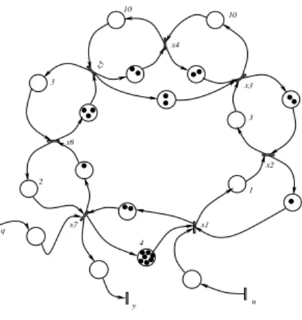
mx3(k + 1) = x3(k + 1) ⊕ x5(k − 1). (19) The resulting graph modification involves adding a single place with two tokens from transition x5 to transition x3. State modification driven by Eq. (19) leads to the supervisor represented in figure 6. This supervision involves imposing only two tokens in the circuit x3 → x5 → x3 which corresponds to the IO cells of the plant (figure 1), that is, the whole furnace (heating and cooling zone). It is easy to check that if we do this, no product will remain more than10 time units in the heating zone of the furnace because there will be a free place in the cooling zone. This supervision guarantees that parts (a maximum of two parts) entering the furnace cannot be lost even when saturation occurs at the evacuation station. x5 x2 x7 x3 x4 x6 x1 q u y 4 1 3 10 10 3 2
Fig. 6. First supervision.
In a similar way, we can obtain other supervisors from Eq. (19) and by taking into account other equations of Eq. (1) (for commandability reasons). Indeed, from the fifth equation of Eq. (1), we havex5(k −1) = 10x4(k −1)⊕x6(k −4). In this equation,10x4(k − 1) represents the normal incrementation of the process due to the dynamic behaviour of the TEG, and x6(k − 4) represents availability of a resource (conveying to the unloading station). Non-evacuation of a part treated affects the availability of the resource: there is no more place at the unloading station to receive new parts and treated parts accumulate in the conveyor. It follows that x5(k − 1) = x6(k − 4). From this latter equation and Eq. (19), we thus obtain the state modification:
mx3(k + 1) = x3(k + 1) ⊕ x6(k − 4). (20) This new supervision involves adding a single place with five tokens from transitionx6 to transitionx3. This leads to the supervision presented in figure 7. The supervisor imposes a maximum of five tokens in circuit x3 → x6 → x3. Thus,
imposing five tokens in this circuit makes it possible to guarantee that no parts will remain more than10 time units in the heating zone: five places are available in the circuit x4→ x6→ x4. x5 x2 x7 x3 x4 x6 x1 q u y 4 1 3 10 10 3 2
Fig. 7. Second supervision.
Finally, and in a similar way, a third supervisor is cal-culated from Eq. (20) and the sixth equation of Eq. (1). Indeed, we have x6(k − 4) = 3x5(k − 4) ⊕ x7(k − 5), where 3x5(k − 4) represents the normal incrementation of a process due to the dynamic behaviour of the TEG and x7(k −5) represents availability of a resource (unloading op-erator). Non-evacuation of treated parts only affects resource availability and it follows thatx6(k − 4) = x7(k − 5). We thus obtain from this equation and Eq. (20) the corresponding state modification:
mx3(k + 1) = x3(k + 1) ⊕ x7(k − 5). (21) By proceeding in this way, the supervision involves imposing six tokens in circuit x3 → x7 → x3. The supervision obtained is given in figure 8.
x5 x2 x7 x3 x4 x6 x1 q u y 4 1 3 10 10 3 2
Fig. 8. Third supervision.
D. Classification of supervisors
This section discusses the classification of supervisors synthesised in section IV-C. Classification is addressed by comparing the production throughput yielded by systems
“TEG+supervisor”, in comparison to the production through-put of the non-supervised manufacturing unit. For this pur-pose, we compute cycle times associated with the TEGs of figures 2, 6, 7 and 8. Recall that the cycle time is the inverse of the production throughput.
Letλ be the cycle time of the non-supervised manufactur-ing unit (figure 2). The followmanufactur-ing procedure (see [8] or [17]) makes it easy to determine λ: for every circuit i (sequence of vertices and arcs which allows a direct connection fromi toi) of the graph, determine the ratio
λi=
Sum of cycle temporisations
Number of tokens in the cycle. (22) Then,λ is the maximum of λi.
From the above procedure, the cycle time of the non-supervised unit is:
λ = max{33 7 , 1 1, 3 2, 10 2 , 10 2 , 3 3, 2 1, 0 13} = 5, (23) and the cycle times are λ�
max{λ, 20/2} = 10, λ�� = max{λ, 23/5} = 5 and λ���
= max{λ, 25/6} = 5 of the unit supervised according to figures 6, 7 and 8 respectively.
The cycle time λ�
of the supervised TEG of figure 6 is greater thanλ. Thus, the supervision represented in figure 6 affects the production throughput of the industrial plant. In contrast, λ��
= ��
= λ: supervisors represented in figures 7 and 8 preserve the initial production throughput of the industrial plant. Comparing the TEGs in figures 7 and 8, the cycle time yielded by adding the supervisor’s place, are23/5 and 25/6, but both supervisors lead to the same resulting throughput for the plant and they are therefore equivalent according to production throughput criteria.
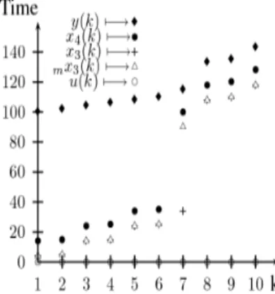
In order to illustrate the plant functioning with and without supervision, assume that the unloading operator may not be present before 100 time units have passed. Figure 9 shows the firing of transitions u, x3, x4, and y for the non-supervised plant and mx3 replaces x3 for the supervised plant, with the third supervisor (figure 8). We observe that the delay between firingx3(7) and x4(7) is 86 for the non-supervised plant: products are lost, while supervision ensures that the time constraint is met, which is 10 time units in the place that links transitionsmx3(k) to x4(k).
V. CONCLUSION
This paper presents a method for the supervision of a manufacturing plant subject to strict time constraints. The method proposed involves injecting the constraint in the state equation of the TEG model associated with the plant and solving the constrained state equation just obtained. This analysis makes it possible to synthesise supervisors aimed at guaranteeing maximum duration constraints. In order to classify supervisors, the use of performance criterion such as the cycle time could be considered. The approach used in this work for a specific TEG can be extended by considering general states and time constraint expressions. This generalisation will be addressed in future work.
Fig. 9. Behaviour of the plant in both unsupervised and supervised cases.
Note that the duration between firings of x3(7) and x4(7) exceeds the
time constraints (10 time units) in the case of the non-supervised plant.
This problem no longer exists for the supervised plant (mx3(7))
REFERENCES
[1] C. Martinez and P. Castagna, “Sizing of an industrial plant using tight
time constraints using complementary approaches:(max, +) theory
and computer simulation,” Elsevier, Simulation Practice and Theory, vol. 11, pp. pp 75–88, 2003.
[2] S. Amari, I. Demongodin, J. Loiseau, and C. Martinez, “Sizing and cycle time of an industrial plant using dio¨ıd algebra,” t. M. on Advanced Computer Systems Production System Design Supply Chain Management (ACS’02-SCM), Ed., 2002, pp. pp 99–106. [3] C. Cassandras and S. Lafortune, Introduction to discrete event systems,
K. Academic, Ed. Kluwer Academic, 1992.
[4] S. Gaubert, “Th´eorie des syst´emes lin´eaires dans les dio¨ıdes,” Ph.D.
dissertation, ´Ecole des Mines de Paris, 1992.
[5] T. Murata, “Petri nets: Properties, analysis and applications,” I. Pro-ceedings, Ed., vol. 77, no. 4, 1989, pp. pp 541–580.
[6] F. Baccelli, G. Cohen, G. Olsder, and J. Quadrat, Synchronization and
Linearity, Wiley, Ed. Wiley, 1992.
[7] G. Cohen, P. Moller, J. Quadrat, and M. Viot, “Algebraic tools for the performance evaluation of discrete event systems,” I. P. S. issue on Discrete Event Systems, Ed., 1985.
[8] G. Cohen, D. Dubois, J. Quadrat, and M. Viot, “Analyse du com-portement p´eriodique des syst`emes de production par la th´eorie des dio¨ıdes,” INRIA, Tech. Rep. 191, 1983.
[9] S. Gaubert, “Resource optimization and (min,+) spectral theory,” IEEE Trans. on Automatic Control, vol. 40, no. 11, pp. pp 1931–1934, 1995. [10] P. Spacek, M. Manier, and A. Moudni, “Control of an electroplating line in the max and min algebras,” International Journal of Systems Science, vol. 30, no. 7, pp. pp 759–778, 1999.
[11] J. Kim and T. Lee, “Schedule stabilization and robust timing control for time-constrained cluster tools,” I. I. C. on Robotics and T. Au-tomation, Taipei, Eds., 2003, pp. pp 1039–1044.
[12] S. Amari, J. Loiseau, and I. Demongodin, “Control of linear min-plus systems under temporal constraints,” t. I. C. on Decision, Control, and S. the European Control Conference 2005, Seville, Eds., 2005, pp. pp 7738–7743.
[13] L. Houssin, S. Lahaye, and J. Boimond, “Just in time control of con-strained (max, +)-linear systems,” Journal of Discrete Event Dynamic Systems, vol. 17, pp. pp 159–178, 2007.
[14] G. Cohen, “Dioids and discrete event systems,” in Lect. Notes. in Control and Inf. Sci, P. of the 11th Conf. on Anal. and O. of Systems:
Discrete Event Systems, Eds., no. 199. Springer, Sophia Antipolis,
1994.
[15] L. Libeaut, “Sur l’utilisation des dio¨ıdes pour la commande des syst`emes `a ´ev´enements discrets,” Ph.D. dissertation, ECN - Universit´e de Nantes, 1996.
[16] C. Commault, “Feedback stabilisation of some event graph models,” IEEE Trans. on Automatic Control, 1998.
[17] H. Hillion and J. Proth, “Performance evaluation of job-shopsystems using timed event-graphs,” IEEE Trans. on Automatic Control, vol. 34, no. 1, pp. 3–9, 1989.