Measuring atmospheric CO₂ from space using Full Spectral Initiation (FSI) WFM-DOAS

HAL Id: hal-00296010

https://hal.archives-ouvertes.fr/hal-00296010

Submitted on 30 Aug 2006

HAL is a multi-disciplinary open access

archive for the deposit and dissemination of

sci-entific research documents, whether they are

pub-lished or not. The documents may come from

teaching and research institutions in France or

abroad, or from public or private research centers.

L’archive ouverte pluridisciplinaire HAL, est

destinée au dépôt et à la diffusion de documents

scientifiques de niveau recherche, publiés ou non,

émanant des établissements d’enseignement et de

recherche français ou étrangers, des laboratoires

publics ou privés.

Spectral Initiation (FSI) WFM-DOAS

M. P. Barkley, U. Frieß, P. S. Monks

To cite this version:

M. P. Barkley, U. Frieß, P. S. Monks. Measuring atmospheric CO2 from space using Full Spectral

Initiation (FSI) WFM-DOAS. Atmospheric Chemistry and Physics, European Geosciences Union,

2006, 6 (11), pp.3517-3534. �hal-00296010�

www.atmos-chem-phys.net/6/3517/2006/ © Author(s) 2006. This work is licensed under a Creative Commons License.

Chemistry

and Physics

Measuring atmospheric CO

2

from space using Full Spectral

Initiation (FSI) WFM-DOAS

1_{EOS, Space Research Centre, Department of Physics & Astronomy, University of Leicester, Leicester, LE1 7RH, UK}

2_{Department of Chemistry, University of Leicester, Leicester, LE1 7RH, UK}

*_{now at: Institute of Environmental Physics, Heidelberg, Germany}

Received: 6 December 2005 – Published in Atmos. Chem. Phys. Discuss.: 10 April 2006 Revised: 26 June 2006 – Accepted: 24 August 2006 – Published: 30 August 2006

Abstract. Satellite measurements of atmospheric CO2

con-centrations are a rapidly evolving area of scientific research which can help reduce the uncertainties in the global car-bon cycle fluxes and provide insight into surface sources

and sinks. One of the emerging CO2 measurement

tech-niques is a relatively new retrieval algorithm called Weight-ing Function Modified Differential Optical Absorption Spec-troscopy (WFM-DOAS) that has been developed by Buch-witz et al. (2000). This algorithm is designed to measure the

total columns of CO2(and other greenhouse gases) through

the application to spectral measurements in the near infrared (NIR), made by the SCIAMACHY instrument on-board EN-VISAT. The algorithm itself is based on fitting the logarithm of a model reference spectrum and its derivatives to the log-arithm of the ratio of a measured nadir radiance and so-lar irradiance spectrum. In this work, a detailed error as-sessment of this technique has been conducted and it has been found necessary to include suitable a priori information within the retrieval in order to minimize the errors on the

retrieved CO2columns. Hence, a more flexible

implementa-tion of the retrieval technique, called Full Spectral Initiaimplementa-tion (FSI) WFM-DOAS, has been developed which generates a reference spectrum for each individual SCIAMACHY obser-vation using the estimated properties of the atmosphere and surface at the time of the measurement. Initial retrievals over Siberia during the summer of 2003 show that the measured

CO2columns are not biased from the input a priori data and

that whilst the monthly averaged CO2distributions contain a

high degree of variability, they also contain interesting spa-tial features.

Correspondence to: P. S. Monks

(psm7@le.ac.uk)

1 Introduction

The carbon cycle is one of the most important physical sys-tems on the Earth and its response to increased levels of

atmospheric CO2 and to global warming is one of the

fac-tors that will shape the future climate. In the natural cycle, carbon is continually transported between the atmosphere, ocean and terrestrial biosphere through fluxes that are of or-der of tens of billion tons per year (Intergovernmental Panel on Climate Change, 2001). Over the last 200 years humans have perturbed this natural cycle by adding comparatively small, but nevertheless significant amounts of carbon into the atmosphere through the burning of fossil fuels, deforestation and by the industrial production of cement, lime and ammo-nia. Consequently during this period the concentration of

atmospheric CO2has risen by about 30%, soaring from 270

to 370 ppmv (parts per million by volume). Only approxi-mately half of the total anthropogenic carbon emitted into the atmosphere actually remains there, the rest being absorbed by the oceans and terrestrial biosphere (Sabine et al., 2004). Carbon that eventually reaches the deep oceans is considered to be removed from the climate system for several hundred years whereas that sequestered by the biosphere may subse-quently be released back to the atmosphere over much shorter timescales. The variability and efficiency of the oceanic and terrestrial fluxes will therefore be critical in determining

fu-ture atmospheric CO2levels.

Currently these fluxes are estimated using inverse meth-ods that employ transport models coupled with surface mea-surements of the atmospheric concentration (e.g. R¨odenbeck et al., 2003). However, such models are hampered firstly by the accuracy of the meteorological fields that drive them and secondly by the sparseness and inhomogeneous

geo-graphical distribution of the approximately one hundred CO2

measurement sites that provide the observational constraints

(GLOBALVIEW-CO2, 2005). Although this approach firmly

1990; Ciais et al., 1995), it is somewhat limited as it cannot fully resolve the North American and Eurasian components nor can it determine the extent of the fluxes in the South-ern Oceans (Gurney et al., 2002). Knowledge of such re-gional scale fluxes and the processes that control them can be vastly improved through sampling the atmosphere more comprehensively. The optimal way to achieve this is to make observations from space.

However, this is a challenging observational problem as

CO2 is considered to be well mixed within the atmosphere

owing to its long lifetime. As it is chemically inert, its dis-tribution is influenced by transport processes and through the spatial and temporal variability of both natural and anthro-pogenic surface fluxes. Seasonal and geographical trends and gradients are evident, not only at the surface but also within the free troposphere and lower stratosphere, typically with an observed variability of about 1–20 ppmv (Nakazawa et al., 1991, 1992; Conway et al., 1994; Anderson et al., 1996; Nakazawa et al., 1997; Vay et al., 1999; Kuck et al., 2000; Levin et al., 2002; Matsueda et al., 2002; Sidorov et al.,

2002). That aside, total columns of CO2exhibit about only

half the variability at the surface with the diurnal fluctuations rarely exceeding 1 ppmv (Olsen and Randerson, 2004). Such

small fluctuations in the CO2concentration will only

there-fore produce correspondingly small changes in radiance at the top of the atmosphere (Mao and Kawa, 2004). Since carbon dioxide is a strong absorber, any space-borne sensor will need to detect such minor responses against what is a dominant background signal. The detection of small radi-ance changes against this strong background requires mea-surements to be made at high precision, challenging the in-strumental limits of the current suite of available sensors. If satellite observations are to improve over the existing ground network, monthly averaged column data at a precision of 1% (2.5 ppmv) or better, for an 8◦×10◦footprint are needed (Rayner and O’Brien, 2001).

Over the last several years various sensitivity analyses have been undertaken to assess if this 1% precision is

at-tainable by satellite instruments. These have mostly

fo-cussed on the retrieval of total columns from either the near infrared (NIR) using differential absorption optical spec-troscopy (DOAS) (Dufour and Br´eon, 2003; Buchwitz and Burrows, 2004; Buchwitz et al., 2005b) or from the close

ex-amination of the CO2emission bands in the thermal infrared

(Ch´edin et al., 2003). Light in the thermal IR originates from the mid-troposphere in contrast to the reflected sunlight of the near infrared. Thus the near surface sensitivity of the NIR makes it the ideal spectral region for observing surface fluxes (even though the absorption bands at 4 µm and 15 µm are much stronger). In addition the NIR is less sensitive to temperature and water vapour.

Since the launch of the SCIAMACHY instrument on-board the European ENVISAT satellite, there is now an

ability to measure total columns of CO2 and other

green-house gases from spectral measurements in the NIR.

SCIA-MACHY CO2 retrievals have been performed initially by

Buchwitz et al. (2005b), using a relatively new retrieval al-gorithm called “Weighting Function Modified Differential Optical Absorption Spectroscopy” (WFM-DOAS) and also by Houweling et al. (2005) using the Iterative Maximum Likelihood Method (IMLM), (Schrijver, 1999). In this pa-per the SCIAMACHY/WFM-DOAS approach is used but developed further with the aim of increasing the precision

and accuracy of space-borne CO2 retrieval. An initial

as-sessment of this algorithm’s sensitivity is given, highlighting the necessity for the inclusion of suitable a priori informa-tion within the retrieval in order to constrain the errors on

the retrieved CO2columns. Furthermore, a modified

WFM-DOAS CO2retrieval algorithm called “Full Spectral

Initia-tion” (FSI) WFM-DOAS is introduced that uses the known properties of the atmosphere and surface at the time of the SCIAMACHY observation to obtain the best linearization point for each retrieval.

The structure of this paper is as follows. In Sect. 2

the SCIAMACHY instrument is briefly described before the WFM-DOAS retrieval technique and an error assessment of its performance is discussed in Sect. 3. In Sect. 4 the FSI WFM-DOAS retrieval algorithm is introduced with some ini-tial results shown in Sect. 5. The paper finishes with a sum-mary in Sect. 6.

2 The SCIAMACHY instrument

The SCanning Imaging Absoprtion spectroMeter for Atmo-spheric CHartographY (SCIAMACHY) is a passive hyper-spectral UV-VIS-NIR grating spectrometer (Bovensmann et al., 1999). It was launched onboard the ENVISAT satel-lite in March 2002 into a polar sun-synchronous orbit, cross-ing the Equator on its descendcross-ing node (i.e. southwards) at 10:00 a.m. local time. The instrument covers the spec-tral range 240–2380 nm, non-continuously, in eight separate channels, with a moderate resolution of 0.2–1.4 nm. From its orbit, SCIAMACHY can observe the Earth from three dis-tinct viewing geometries nadir, limb and lunar/solar occul-tation, with the majority of the orbit consisting of measure-ments in an alternating limb and nadir sequence. The total

columns of CO2are derived from nadir observations in the

NIR, focussing on a small wavelength window within

chan-nel six, centered on the CO2band at 1.57 µm. The radiation

in this wavelength interval consists of solar energy either re-flected from the surface or scattered from the atmosphere. In nadir mode, the atmosphere directly below the sensor is viewed producing retrievals with good spatial but poor ver-tical resolution. A characteristic set of observations consists of the nadir mirror scanning across track for 4 s followed by a fast 1 s back-scan. This is repeated for either 65 or 80 s according to the orbital region. The ground swath viewed

has fixed dimensions of 960×30 km2, (across × along track).

is 60×30 km2, corresponding to an integration time of 0.25 s. Global coverage is achieved at the Equator within 6 days.

3 Assessment of the WFM-DOAS retrieval algorithm

3.1 WFM-DOAS

The WFM-DOAS algorithm (Buchwitz et al., 2000; Buch-witz and Burrows, 2004) defined in Eq. (1), is based on a linear least squares fit of the logarithm of a model reference spectrum I_irefand its derivatives, plus a quadratic polynomial

Pi, to the logarithm of the measured sun normalized intensity

I_imeas. ln I_imeas(Vt) − " ln I_iref( ¯V) + ∂ln I ref i ∂ ¯VCO2 ·( ˆVCO2 − ¯VCO2) +∂ln I ref i ∂ ¯VH2O ·( ˆVH2O− ¯VH2O) + ∂ln I_iref ∂ ¯VTemp ·( ˆVTemp− ¯VTemp) +Pi(am) # 2

≡ kRESik2 → min w.r.t ˆVj & am (1)

The subscript i refers to each detector pixel of wavelength λi

and the true, model and retrieved vertical columns are repre-sented by Vt=(V_CO2t , V_H2t _O, V_Tempt ), ¯V=( ¯VCO2, ¯VH2O, ¯VTemp)

and ˆVj respectively (where subscript j refers to the variables

CO2, H2O and temperature). Here VTempis not a vertical

col-umn as such, but rather a scaling factor applied to the vertical temperature profile. Each derivative (or column weighting function) represents the change in radiance as a function of a relative scaling of the corresponding trace gas or temperature profile. Effectively the column weighting functions are re-placing the absorption cross sections found in normal DOAS methods. In order to retrieve carbon dioxide derivatives for CO2, H2O and (optionally) temperature are required. In the

case of the temperature derivative, the term ( ˆVTemp− ¯VTemp)

represents the scaling difference of the entire temperature profile. The fit parameters are the trace gas columns ˆVCO2

and ˆVH2O, the temperature scaling factor ˆVTempand the

poly-nomial coefficients am.

Although an initial error analysis was performed by Buch-witz and Burrows (2004) a more thorough study has been conducted, and summarized here, to assess possible biases and retrieval errors. It is not the aim of this paper to repeat their efforts but rather to highlight the most important sources of inaccuracy. To achieve this, synthetic measurements for a given atmospheric state and instrument set-up were gener-ated using the radiative transfer model SCIATRAN (Rozanov et al., 2002). Simulated retrievals were then performed using a standard reference spectrum, so that in each case the

re-trieved CO2column could be compared to its true value. This

reference spectrum was constructed using the U.S. Standard

atmosphere (McClatchey et al., 1972) together with a default

aerosol scenario (unless indicated otherwise). The CO2

pro-file was scaled to coincide with its current concentration of 370 ppmv. Aerosols were parameterized by the LOWTRAN scheme (Kneizys et al., 1986, 1996) the default setting being a spring/summer season with maritime aerosols in the bound-ary layer (visibility 23 km and humidity 80%). Background tropospheric and stratospheric aerosol conditions were as-sumed in conjunction with a normal mesospheric loading. Both the solar zenith and the relative azimuth angles (both 45◦) and the albedo at 0.2 were kept constant throughout the studies (unless indicated). Each spectrum was created on a high resolution wavelength grid and then convolved with a Gaussian slit function of 1.4 nm (FWHM) before being in-terpolated onto the SCIAMACHY wavelength grid. The fit-ting window used throughout this sensitivity analysis was confined to the wavelength region 1561.03–1585.39 nm (see

Sect. 4) which, besides the CO2band, contains some weak

water vapour absorption lines. Weighting functions for CO2

and H2O, together with the quadratic polynomial were

al-ways included in the WFM-DOAS fit. However for each scenario the simulated retrieval was performed both with and without the temperature weighting function, thus allowing its contribution to be assessed. In this sensitivity study, the relative column error Erel, that is the percentage difference

between the retrieved CO2column ˆVCO2 and the actual

col-umn V_COt

2, is used to gauge the accuracy of each simulated

retrieval (Eq. 2). Erel= ˆ VCO2−V t CO2 V_COt 2 ×100% (2)

3.2 Sensitivity to CO2vertical profile

The CO2 profile associated with the U.S. Standard

atmo-sphere has a uniform volume mixing ratio of 370 ppmv, up to an altitude of 80 km. For the tropical regions, where ver-tical mixing is rapid, this is a fair representation. For higher latitudes however, the shape of the profile is more strongly influenced by dynamics and biospheric activity thus varying seasonally (Anderson et al., 1996; Nakazawa et al., 1997). To ascertain the sensitivity of the algorithm to the vertical

CO2distribution, simulated retrievals were performed using

spectra generated from profiles more representative of the global latitudinal and seasonal CO2 distribution (illustrated

in Fig. 1), taken from a newly prepared climatology

(Reme-dios et al., 2006). In each simulation the CO2 profile was

interpolated onto the U.S. Standard pressure scale and used in conjunction with the U.S. Standard temperature and water vapour profiles.

The results from these simulations show that the shape of

the CO2 profile used to create the model reference spectra

is important (Fig. 2). Using a uniform CO2profile tends to

lead to an over-estimation of the true CO2concentration

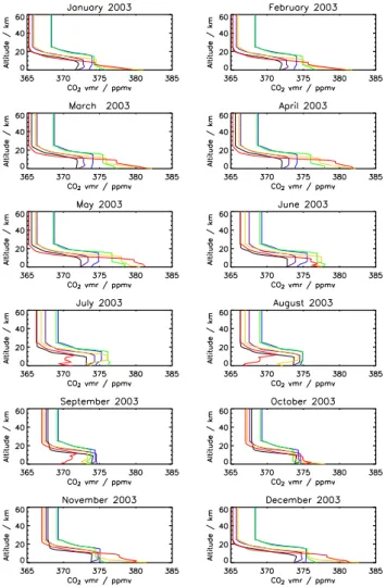
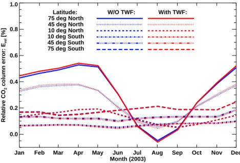
Fig. 1. Vertical CO2profiles used in the sensitivity analysis. This data set, for 2003, contains a total of 72 CO2profiles, constructed from the flask measurements made by the GLOBALVIEW network. Each month has six profiles centered on the latitudes 75◦N (red), 45◦N (yellow), 10◦N (green), 10◦S (blue), 45◦S (purple) and 75◦S (black), each representative of a 30◦latitude band.

relative error in the retrieved column varies throughout the year and is most pronounced in the Northern Hemisphere where it follows the seasonal cycle, peaking in the month

of April at ∼0.5%. In the Southern Hemisphere, where

the CO2distribution is dominated by inter-hemispheric

mix-ing, this seasonal variation is not observed and the error is smaller, typically less than 0.2%. Failure to use realistic a

priori CO2 vertical profiles within the WFM-DOAS

algo-rithm will therefore introduce time-dependent biases. How-ever, for SCIAMACHY and model comparisons, this bias can be minimized by applying an averaging kernel correc-tion to the model data (see, e.g. Barkley et al., 2006). The WFM-DOAS averaging kernels, which peak in the planetary boundary layer, highlight the sensitivity of SCIAMACHY to the lower troposphere (see Buchwitz et al., 2005a).

3.3 Sensitivity to temperature and water vapour profiles

The U.S. standard atmosphere, used to generate the baseline scenario, represents an average climatology whereas the real environment itself is obviously more varied especially be-tween the distinct latitude bands of the tropics, mid latitudes and sub-polar regions. Water vapour and temperature profiles representative of these areas (McClatchey et al., 1972) were consequently used to produce a series of simulated measure-ments in a similar manner to Buchwitz and Burrows (2004). However, to create a much wider range of atmospheric states both the CO2and H2O trace gas profiles were also multiplied

by constant factors (where the CO2profile here, refers to that

of the U.S. Standard atmosphere). In an addition to this, a further set of simulated measurements was created from 16 ECMWF (un-scaled) temperature and water vapour profiles selected from the months of January and July 2003. These were chosen on the basis of being strongly deviant from the U.S. standard atmosphere (see Fig. 3).

These simulations reveal that the accuracy of the retrieved

CO2column is highly dependent on the inclusion of the

tem-perature weighting function within the WFM-DOAS fit. If the temperature derivative is included, then in the case of the regional profiles (Table 1) the errors are less than 1% even

when there is coincidental uniform scaling of the CO2

pro-file. These results are consistent to those presented in Buch-witz and Burrows (2004). When more realistic ECMWF pro-files are used to generate the synthetic measurements, these errors are larger typically <1.5%, without any additional

scaling of the CO2concentration (Table 2). Using a

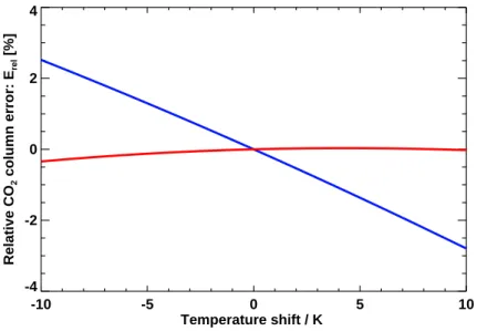
clima-tological mean profile to produce the baseline spectrum is hence inadequate, suggesting that a priori knowledge of the temperature and water vapour profiles is needed when apply-ing WFM-DOAS to real SCIAMACHY spectra. Even if the reference spectra are created from assimilated atmospheric profiles, the temperature derivative must always be included within the retrieval to limit this source of error. This is also clearly demonstrated by examining the retrieval around the temperature linearization point. To accomplish this, a third set of synthetic measurements was created by applying small temperature shifts of 1 K to the U.S. Standard atmosphere (up to a maximum of ±10 K). The subsequent retrievals re-veal that not fitting the temperature derivative can produce a

relative error in the CO2column of as much as ±1.3% for

a uniform ±5 K difference between the true and reference temperature profiles (Fig. 4). If the temperature weighting function is fitted, this error is kept to less than 0.1%.

3.4 Sensitivity to the combined effect of using alternative

CO2, H2O and temperature vertical profiles

Sections 3.2 and 3.3 have shown that sufficient knowledge

of the CO2, temperature and water vapour profiles is

nec-essary to produce accurate retrievals. It is possible to

Table 1. Relative errors produced in the retrieved CO2column created from using alternative temperature and water vapour profiles. Scaling factors of 0.95, 0.97, 1.0, 1.03 and 1.05 applied to the CO2column yield mixing ratios of 351.5 ppmv, 358.9 ppmv, 370 ppmv, 381.1 ppmv and 388.5 ppmv respectively. No TWF: temperature weighting function not fitted. TWF: temperature weighting function fitted.

Climatology Water vapour Relative column error (%)

Scaling CO2Column scaling

0.95 0.97 1.00 1.03 1.05 No TWF TWF No TWF TWF No TWF TWF No TWF TWF No TWF TWF 0.5 −2.72 −0.29 −2.68 −0.26 −2.66 −0.25 −2.68 −0.28 −2.71 −0.32 Tropical 1.0 −2.78 −0.32 −2.73 −0.29 −2.70 −0.28 −2.71 −0.30 −2.74 −0.34 1.5 −3.03 −0.46 −2.98 −0.42 −2.94 −0.40 −2.94 −0.42 −2.96 −0.45 0.5 −3.17 −0.82 −3.00 −0.67 −2.79 −0.49 −2.64 −0.37 −2.56 −0.32

Mid Lat Summer 1.0 −3.20 −0.84 −3.02 −0.69 −2.81 −0.51 −2.65 −0.39 −2.57 −0.33

1.5 −3.35 −0.94 −3.17 −0.78 −2.94 −0.60 −2.78 −0.47 −2.70 −0.40

0.5 1.69 −0.04 1.86 0.12 2.06 0.31 2.20 0.45 2.26 0.52

Mid Lat Winter 1.0 1.68 −0.05 1.85 0.11 2.05 0.31 2.19 0.45 2.26 0.51

1.5 1.66 −0.06 1.83 0.11 2.03 0.30 2.17 0.44 2.24 0.51

0.5 −1.57 −0.54 −1.40 −0.39 −1.18 −0.20 −1.03 −0.07 −0.95 −0.01

Sub Arc Summer 1.0 −0.02 −0.57 −1.42 −0.41 −1.20 −0.22 −1.04 −0.08 −0.96 −0.02

1.5 −1.70 −0.63 −1.51 −0.47 −1.29 −0.28 −1.12 −0.13 −1.04 −0.07

0.5 3.74 −0.31 3.91 −0.13 4.11 0.08 4.26 0.23 4.33 0.32

Sub Arc Winter 1.0 3.73 −0.31 3.90 −0.13 4.11 0.08 4.25 0.24 4.32 0.32

1.5 3.72 −0.31 3.89 −0.13 4.10 0.08 4.26 0.24 4.32 0.32

Table 2. The relative column error produced in the retrieved CO₂column brought about from using ECMWF temperature and water vapour profiles instead of the U.S. Standard atmosphere. Each ECMWF profile number corresponds to the indexing in Fig. 3. The first and second columns show the error from using the temperature and water vapour profiles individually whilst the final column shows their combined effect.

Temperature Water Vapour Total Error [%] Error % Error % ECMWF Profile No TW TW No TW TW No TW TW 1 1.02 −0.70 0.00 0.00 1.04 −0.70 2 0.98 −0.75 0.00 0.00 1.01 −1.50 3 3.27 0.93 −0.03 −0.02 3.31 0.90 4 3.81 1.16 −0.03 −0.02 3.86 1.17 5 4.81 −0.88 −0.04 −0.01 4.87 −0.89 6 5.19 −0.47 −0.04 −0.02 5.26 −0.48 7 −3.78 −1.13 −0.47 −0.27 −3.99 −1.24 8 2.33 0.93 −0.04 −0.01 2.35 0.94 9 −4.10 −1.33 −0.07 −0.03 −4.04 −1.29 10 −3.16 −1.28 −0.25 −0.15 −4.00 −1.31 11 −3.79 −1.15 −0.40 −0.22 −3.96 −1.24 12 −2.57 −0.39 0.03 0.01 −2.57 −0.39 13 −2.43 −0.32 0.03 0.01 −2.43 −0.32 14 −2.63 −0.39 0.02 0.01 −2.66 −0.41 15 −2.77 −0.27 −0.03 −0.02 −2.72 −0.24 16 −2.80 −0.28 −0.03 −0.02 −2.74 −0.25

Jan Feb Mar Apr May Jun Jul Aug Sep Oct Nov Dec Month (2003) 0.0 0.2 0.4 0.6 0.8 1.0 Relative CO 2 column error: E rel [%]

Latitude: W/O TWF: With TWF: 75 deg North 45 deg North 10 deg North 10 deg South 45 deg South 75 deg South

Fig. 2. The relative errors in the retrieved CO2column for 75◦N (solid), 45◦N (dotted), 10◦N (dashed), 10◦S (dash dot), 45◦S (dash dot dot) and 75◦S (long dashes) produced by using CO2profiles other than the U.S. Standard atmosphere (associated with the reference spectrum), with the simulated retrievals performed both with (red) and without (blue) the temperature weighting function.

180 200 220 240 260 280 300 320 Temperature / K 0 10 20 30 40 50 60 Altitude / km 10 100 1000

H2O Volume mxing ratio / ppmv

0 10 20 30 40 50 60 Altitude / km Profile: 1 Profile: 2 Profile: 3 Profile: 4 Profile: 5 Profile: 6 Profile: 7 Profile: 8 Profile: 9 Profile: 10 Profile: 11 Profile: 12 Profile: 13 Profile: 14 Profile: 15 Profile: 16

Fig. 3. The ECMWF temperature profiles (left) and corresponding water vapour profiles (right) used in the sensitivity analysis, together with the U.S. standard atmosphere (black dashed line).

atmospheric profiles by interpolating the CO2profiles, from

the new climatology (Sect. 3.2), onto the appropriate tropi-cal, mid-latitude and sub-arctic regional profiles. The conse-quent simulations show that relative errors, in the retrieved columns, on the order of 0.5% can be produced (Fig. 5). Un-like the analysis in Sect. 3.2, the temperature derivative has a

much bigger effect. Whilst in the tropics these errors are al-most constant throughout the year, at mid and high latitudes they vary seasonally. During the winter months the mid-latitude columns are systematically overestimated by about 0.75% as compared to the summer where they are underesti-mated by an average of 0.13%. These biases will increase

-10 -5 0 5 10 Temperature shift / K -4 -2 0 2 4 Relative CO 2 column error: E rel [%]

Fig. 4. The sensitivity of the WFM-DOAS algorithm to the temperature linearization point, shown here as a temperature shift of the U.S. Standard Atmosphere, for simulations performed both with/without (red/blue) the temperature weighting function.

Jan Feb Mar Apr May Jun Jul Aug Sep Oct Nov Dec

Month (2003) -4.0 -2.0 0.0 2.0 4.0 6.0 8.0 Relative CO 2 column error: E rel [%]

Latitude Band : W/O TWF: With TWF: Sub-arctic

Mid-latitude Tropics

Fig. 5. The relative column error produced by using realistic monthly CO2profiles and temperature and water vapour profiles represen-tative of the Northern Hemisphere tropics (dotted), mid-latitudes (solid) and sub-arctic (dashed), for simulated retrievals performed both with/without (red/blue) the temperature weighting function.

if the CO2 profiles are interpolated onto the more lifelike

ECMWF profiles. Retrievals performed without using real-istic CO2profiles and realistic temperature and water-vapour

profiles will therefore result in the terrestrial biosphere fluxes in the Northern mid-latitudes being overestimated. Since the

natural variability of atmospheric CO2total columns is only

about 3% these errors are not negligible.

3.5 Sensitivity to the surface elevation and pressure

The surface pressure must be carefully considered in any

CO2 retrieval algorithm. Firstly, because gradients in the

atmospheric CO2 concentration created by variations in the

surface topography and low altitude weather systems can often mask those produced by surface fluxes (Kawa et al., 2004) and secondly because the measurement is sensitive to pressure, owing to the broadening of absorption lines

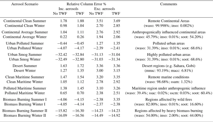
Table 3. Aerosol error analysis. Inc. Aerosols = Simulated retrievals performed using a reference spectrum with the default aerosol scenario. Exc. Aerosols = Simulated retrievals performed using a reference spectrum without any aerosols present. The component contributions are defined as: waso = watersoluble, inso = insoluble, ssam = sea salt accumulation mode, sscm = sea salt coarse mode, mnuc = mineral nucleation mode, macc = mineral accumulation mode. The biomass burning scenarios were taken from Holzer-Popp et al. (2002). The ex-tinction coefficients within the planetary boundary layer (0–2 km) for the urban smog and biomass burning I & II scenarios were 19.49 km−1, 1.50 km−1and 4.00 km−1.

Aerosol Scenario Relative Column Error % Comments Inc. aerosols Exc. aerosols

No TWF TWF No TWF TWF

Continental Clean Summer 1.78 1.88 3.51 3.69 Remote Continental Areas Continental Clean Winter 0.98 1.04 2.70 2.85 (waso: 99.998%; inso: 0.002%) Continental Average Summer 1.04 1.11 2.76 2.92 Anthropogenically influenced continental areas

Continental Average Winter 0.22 0.26 1.94 2.06 (waso: 45.79%; inso: 0.01%; soot: 54.20%) Urban Polluted Summer −0.44 −0.45 1.27 1.35 Polluted urban areas

Urban Polluted Winter −4.07 −4.17 −2.39 −2.41 (waso: 31.39%; inso: 0.01%; soot: 68.6%) Urban Smog Summer −32.42 −32.84 −31.13 −31.04 Highly polluted urban areas

Urban Smog Winter −32.49 −32.80 −31.03 −31.34 (waso: 31.39%; inso: 0.01%; soot: 68.6%) Desert Summer 1.63 1.72 3.36 3.36 Desert regions (e.g. Sahara, Gobi)

Desert Winter 1.27 1.35 3.00 3.15 (mnuc: 93.19%; macc: 6.81%) Clean Maritime Summer 1.47 1.54 3.20 3.35 Remote marine conditions

Clean Maritime Winter 1.05 1.12 2.78 2.92 (waso: 98.68%; ssam: 1.32%) Polluted Maritime Summer 1.38 1.45 3.10 3.26 Maritime region under anthropogenic influence

Polluted Maritime Winter 0.65 0.70 2.38 2.51 (waso: 39.4%; ssac: 0.02%; sscm: 0.03%; soot: 60.4%) Biomass Burning Summer I −4.06 −4.15 −2.38 3.35 Regions affected by wild fires

Biomass Burning Winter I −4.05 −4.14 −2.37 −2.38 (waso: 82.00%; inso: 0.01%; soot: 16.60%) Biomass Burning Summer II −15.82 −16.30 −14.23 −14.23 Regions affected by heavy biomass burning Biomass Burning Winter II −16.09 −16.56 −14.49 −14.92 (waso: 54.00%; inso: 2.00%; soot: 44.00%)

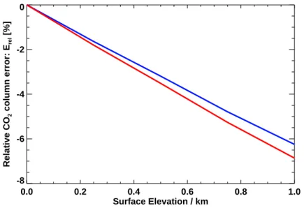
column as a function of the surface pressure was investi-gated by varying the surface elevation within the SCIATRAN model. Inspection of the results (Fig. 6) shows that the re-trieved column is systematically under-estimated when the surface elevation is increased relative to that used in the refer-ence scenario. The magnitude of this error is approximately

−0.31% per 50 m increase in surface elevation, when the

temperature weighting function is not fitted, as opposed to approximately −0.34% per 50 m when it is included. The magnitude of this error is almost identical to that found by Buchwitz et al. (2005b).

3.6 Sensitivity to the surface albedo

The Earths surface reflectance within the near infra-red can vary from as little as 0.001 over the oceans to as much 0.4 over the desert (Dufour and Br´eon, 2003). This affects not only the overall amount of solar radiation reflected back to space (and subsequently the signal to noise ratio of

SCIA-MACHY measurements) but also the relative depth of CO2

and H2O absorption lines by influencing the path-length

trav-eled by the photons (see Buchwitz and Burrows, 2004). To gauge this effect, the column error as a function of the

sur-face reflectance was examined using a reference spectrum produced with an albedo of 0.1 (so as to be consistent with current implementations of WFM-DOAS Buchwitz et al., 2005b). Variations in the surface albedo alone, from 0.05 to 0.4, can cause an error in the retrieved column of up to 2% (Fig. 7). The errors increase further still at very low albedos. This simple test, which doesn’t account for the coupling be-tween the surface reflectance and aerosols (Houweling et al., 2005), demonstrates that employing a fixed albedo within the algorithm will introduce (what are essentially unnecessary) errors.

3.7 Sensitivity to aerosols

Retrievals of CO2 in the near infra-red are affected by the

presence of aerosols (Dufour and Br´eon, 2003). For exam-ple, systematic errors caused by Saharan dust, have already

been clearly identified in CO2columns retrieved from

SCIA-MACHY (Houweling et al., 2005). Aerosols can both scatter and absorb light depending on their composition. Aerosol scattering can either shorten the photon path-length leading

to an underestimation of the CO2 column or alternatively,

path length thereby causing an overestimation (Houweling et al., 2005). To determine their influence on WFM-DOAS, a set of scenarios were created based on the aerosol types defined by Hess et al. (1998) using a parameterization de-veloped by Hoogen (1995). Aerosol extinction profiles were taken (and adapted) from the LOWTRAN library (Kneizys et al., 1996). These aerosols were confined to the boundary layer with background tropospheric and stratospheric condi-tions assumed. Retrievals simulated using the default sce-nario show that the errors are lower than 2%, except in ex-treme cases, and that they increase if the temperature deriva-tive is included within the fit (Table 3). For other surface albedos (other than the default of 0.2) these errors will be different (e.g. Houweling et al., 2005). The background ma-rine conditions associated with the reference spectrum how-ever produces biases when applied to contrasting conditions, for example with urban, biomass burning and desert

scenar-ios. This may have repercussions for trying to estimate CO2

emissions over large urban areas or regions affected by wild fires. However, the inclusion of some background aerosols within the reference spectrum is clearly better than retrievals performed on the basis of an aerosol free atmosphere.

3.8 Fitting of height resolved weighting functions

The non-linearity of DOAS fitting within the near infra-red spectral region, owing to strong absorbers and the effects of pressure broadening, was clearly identified by Frankenberg et al. (2005b). To account for this difficulty, scaling fac-tors for different height layers were used within the IMAP retrieval algorithms constrained state vector. To determine whether the sensitivity of WFM-DOAS could be improved by using a similar approach, the trace gas columns and as-sociated weighting functions of the reference spectrum, were grouped into three individual height layers: 0–3 km, 3–12 km and 12 km to top of the atmosphere (each column derivative being simply the sum of a set of height resolved weighting functions). The simulated retrievals were then repeated using the (unconstrained) weighting functions for the three discrete altitude ranges and the resulting errors compared to those obtained using the original column derivatives. In some in-stances, using this approach did increase the sensitivity of the WFM-DOAS algorithm. However, the results from these simulations were very inconsistent, varying very much on the scenario implemented in each synthetic retrieval. As a result, it is difficult to draw any conclusions regarding this alterna-tive method.

4 Full Spectral Initiation (FSI) WFM-DOAS

The WFM-DOAS algorithm is able to detect changes in the

atmospheric CO2concentration. However if the CO2column

is retrieved using a reference spectrum created from a sce-nario that differs from the true atmospheric state, significant

errors could be introduced. As demonstrated, factors which affect the calculated model spectrum are the surface albedo, surface pressure, aerosols and the vertical profiles of CO2,

water vapour and temperature. When varied alone each of these parameters creates an error in the column of typically less than about 2%. However, in the real atmosphere none are known exactly, thus the errors propagate accordingly and are especially significant when considering the high precision measurements that are needed to observe the small gradients

associated with atmospheric CO2. To reduce these errors a

reference spectrum that is very close to the real measurement must be used, i.e. as much “a priori” information must be included in the retrieval as possible. It is on this basis that a modified retrieval algorithm called Full Spectral Initiation or (FSI)-WFM-DOAS has been developed. In FSI, a refer-ence spectrum is generated for every single SCIAMACHY measurement to obtain the best linearization point for the re-trieval. Subsequent iterations are not performed, in order to limit the computational time. Were this not an issue, then the

retrieved CO2vertical column density would be fed back into

the algorithm iteratively. To calculate the best possible ref-erence spectrum all the known or rather estimated properties of the atmosphere and surface at the time of the observation, serve as input for the radiative transfer model. Once the sun-normalized radiance is obtained, a WFM-DOAS fit is then performed and the vertical column retrieved.

The FSI algorithm is applied to calibrated radiances us-ing the fittus-ing window 1561.03–1585.39 nm. This region was chosen in order to minimize interference from water vapour and not to extend into channel 6+, where the Indium Gal-lium Arsenide (InGaAs) detectors were doped with higher amounts of Indium leading to different behavioural charac-teristics (Lichtenberg et al., 2005). The number of fitting points within this micro-window is usually thirty-two, with each detector pixel spanning a wavelength interval of 0.7 nm. Owing to the broad slit function of this channel (see Sect. 5),

SCIAMACHY does not fully resolve the CO2 absorption

bands. This spectral interval is also advantageous in that, unlike channels 7 and 8, it is unaffected by orbital varia-tions of the dark current and the build up of ice-layers on the detectors (as discussed by Gloudemans et al., 2005). It is also stable with regard to so called “dead and bad pix-els” created by thermal and radiation degradation (Kleipool, 2004). The SCIAMACHY pixel mask however, is checked and if necessary, updated for each orbit using the standard deviations of the dark current, as proposed by Frankenberg et al. (2005a). Detector pixels are also discarded if erro-neous spikes occur in the measured radiance. All measure-ments have been corrected for non-linear effects (Kleipool, 2003b) and the dark current (Kleipool, 2003a). The FSI algo-rithm also uses a solar reference spectrum with improved cal-ibration, provided to the SCIAMACHY community by ESA, courtesy of Johannes Frerick (ESA, ESTEC), in preference to that in the official L1C product. An optimized systematic shift, based on the inspection of the fit residuals, of 0.15 nm

0.0 0.2 0.4 0.6 0.8 1.0 Surface Elevation / km -8 -6 -4 -2 0 Relative CO 2 column error: E rel [%]

Fig. 6. The relative column error produced as a function of the surface elevation, for simulations performed both with/without (red/blue) the temperature weighting function. Here the retrieved CO2column is systematically under-estimated.

0.0 0.1 0.2 0.3 0.4 0.5 0.6 0.7 Surface Albedo [-] -15 -10 -5 0 5 Relative CO 2 column error: E rel [%]

Fig. 7. The relative column error produced as a function of the surface albedo, assuming background maritime aerosols and for a solar zenith angle of 45◦. In this instance the errors produced by fitting (red) and not fitting (blue) the temperature weighting function are barely discernible.

is applied to the observed spectra to align it to the synthetic radiances calculated by SCIATRAN. To improve the qual-ity of the FSI spectral fits, the latest version of the HITRAN molecular spectroscopic database has been implemented in the radiative transfer model (Rothman et al., 2005). Each SCIAMACHY observation has an associated reference spec-trum created from several sources of atmospheric and surface

data. The CO2profile is selected from the new climatology

(Sect. 3.2) and is chosen according to the time of the observa-tion and the latitude band in which the ground pixel falls. To

obtain the closest atmospheric state to the observation tem-perature, pressure and water vapour profiles, derived from

operational 6 hourly ECMWF data (1.125◦_×1.125◦_{grid), are}

interpolated onto the local overpass time and centre of the SCIAMACHY pixel. To determine the linearization point for the surface albedo, a look-up table of mean radiances, for the defined fitting window, has been generated as a func-tion of both the surface reflectance and solar zenith angle. From using the mean radiance of the SCIAMACHY obser-vation and the solar zenith angle at the corresponding time,

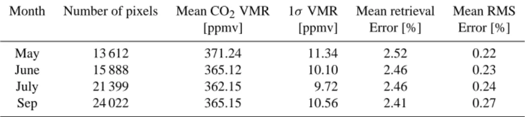
Table 4. Summary of FSI WFM-DOAS retrieval results for the Siberian test region (see Fig. 14) during the summer of 2003. Month Number of pixels Mean CO2VMR 1σ VMR Mean retrieval Mean RMS

[ppmv] [ppmv] Error [%] Error [%] May 13 612 371.24 11.34 2.52 0.22 June 15 888 365.12 10.10 2.46 0.23 July 21 399 362.15 9.72 2.46 0.24 Sep 24 022 365.15 10.56 2.41 0.27

it is possible to infer an approximate value for the albedo. To account for aerosols, three scenarios are incorporated into the retrieval algorithm. Maritime and rural scenarios are imple-mented over the oceans and land respectively. In both cases, the boundary layer visibility is 23 km. If a major city occurs within the SCIAMACHY footprint then an urban scenario is selected with a reduced visibility of 5 km. For all three cases the LOWTRAN aerosol model is employed, with the relative humidity set to 80% in summer and 70% in winter. Background conditions are assumed for the free troposphere, stratosphere and mesosphere. This representation of the local aerosol conditions however, is still quite limited.

The viewing geometry of SCIAMACHY allows it to scan

to ±30◦around the nadir line of sight. Unfortunately every

model spectrum must be calculated for the exact nadir po-sition, as the computational time for off axis spectra is very high. To account for the increased path-length in off-axis viewing geometry, a correction has been be applied to the final retrieved column (Buchwitz et al., 2000). This is not an ideal solution, as it can cause an over correction of up to 2–3% for pixels at the extremities (Buchwitz and Burrows, 2004). All SCIAMACHY observations are cloud screened prior to retrieval processing, with cloud contaminated pixels flagged and disregarded using the current version of the Hei-delberg Iterative Cloud Retrieval Utilities (HICRU) database (Grzegorski et al., 2005). Where gaps occur in this database or if the HICRU algorithm fails then an alternative method is employed which uses the polarization measurement devices, specifically PMD1, flagging a pixel if a pre-defined threshold (set at 70 000 BU) is exceeded (de Beek et al., 2004). Back-scans along with observations that have solar zenith angles

greater than 75◦are also excluded. All columns are

normal-ized to the ECMWF surface pressure to produce a column volume mixing ratio (VMR).

5 Preliminary results

The calculation of a reference spectrum for each SCIA-MACHY observation, whilst felt necessary, is still time-consuming at approximately 5 min per ground pixel. This means that, at this stage, FSI-WFM-DOAS can only be ap-plied to selected “target regions” that are of particular sci-entific interest. In this first demonstration of the FSI

algo-rithm, Siberia has been chosen as an example test region,

specifically the area bounded by the latitudes 48◦_N–80◦_N

and the longitudes of 45◦E–180◦E, with just the summer

months processed (excluding August during which SCIA-MACHY underwent a decontamination phase to remove ice on the NIR detectors). To ensure only valid retrievals are ex-amined, only columns that have retrieval errors less than 5% and lie within a quite broad range of 340–400 ppmv are ac-cepted (column VMRs lying outside this range are likely to originate from undetected clouds or from aerosol scattering). These results are summarized in Table 4. In this initial anal-ysis, comparisons to chemical transport models, for example the TM3 model (Heimann and K¨orner, 2003) or ground sta-tion data are not made, as such data will be used in future research to determine the precision and accuracy of the FSI algorithm (Barkley et al., 2006). Instead the focus is on the quality of the spectral fits and possible errors and biases as-sociated with the FSI WFM-DOAS retrieval. Hence, in this study neither the retrieved columns (in molecules per cm2) or the normalized columns (in ppmv), have had scaling factors applied as in other studies (e.g. Yang et al., 2002 or Buch-witz et al., 2005b), thus only the CO2spatial distribution can

really be discussed.

The spectral fits produced by the FSI algorithm are

promising, with a typical fit shown in Fig. 8. The CO2 fit

indicates that there is good sensitivity to the CO2 vertical

column unlike temperature, where the fit is much worse. If the retrievals are repeated but this time only fitting the CO2

and H2O weighting functions, then the magnitude of the

ver-tical columns increases but their relative spatial distribution remains the same. Fitting the temperature derivative there-fore only creates a negative offset, suggesting that the current algorithm is more sensitive to other factors, possibly calibra-tion issues. Nevertheless, it is always included, following the sensitivity study presented in Sect. 3. By averaging over all retrievals, the mean fit residual should ideally reflect only measurement noise. However, this is not the case, illustrated by Fig. 9, as it contains quite stable systematic structures, the origin of which has yet to be clarified. It is most likely that such features will be reduced (or removed) by improving the calibration of the SCIAMACHY spectra and through contin-ually including the latest spectroscopic data in the radiative transfer model. The residuals are also strongly influenced by the slit function used in the convolution of the reference

Fig. 8. A typical example of a FSI WFM-DOAS fit. Top panel: The reference spectrum (blue) generated by the retrieval (from the a priori data), the sun-normalized radiance measured by SCIAMACHY (black diamonds) and the FSI WFM-DOAS fit (red) to this measurement. Following three panels: (i) The CO2fit. This shows CO2total column weighting function (WF) and the CO2fit residuum (red diamonds), which is the CO2WF plus the difference between the measurement and fit (i.e. the fit residual) (ii–iii) Similar but for H2O and temperature. Bottom panel: The fit residual with a root-mean-square (RMS) difference of 0.13%.

1560 1565 1570 1575 1580 1585 1590 Wavelength [nm] -0.02 -0.01 0.00 0.01 0.02 Residual [-]

Michael Barkley, ULeic. (FSI WFM-DOAS V1)

Mean Residual (Black line)

Fig. 9. FSI WFM-DOAS fit residuals for the Siberian test region during May 2003, over-plotted with the mean fit residual (black). The mean RMS error is 0.22%. The detector pixel, of wavelength 1576.72 nm, is omitted in the retrieval as this always worsens the quality of the fit and increases the error on the retrieved column.

60 80 100 120 140 160 180 Longitude 50 55 60 65 70 75 80 Latitude

CO2 Vertical Column Density [x10 21

molec. cm-2 ]

<6.000 6.375 6.750 7.125 7.500 7.875 8.250 8.625 >9.000

Michael Barkley, ULeic. (FSI WFM-DOAS v1.1) CO2 Climatology

60 80 100 120 140 160 180 Longitude 50 55 60 65 70 75 80 Latitude

CO2 Vertical Column Density [x10 21

molec. cm-2 ]

<6.000 6.375 6.750 7.125 7.500 7.875 8.250 8.625 >9.000

Michael Barkley, ULeic. (FSI WFM-DOAS v1.1) SCIAMACHY NIR (Fitting Window: 1561.03-1585.39 nm)

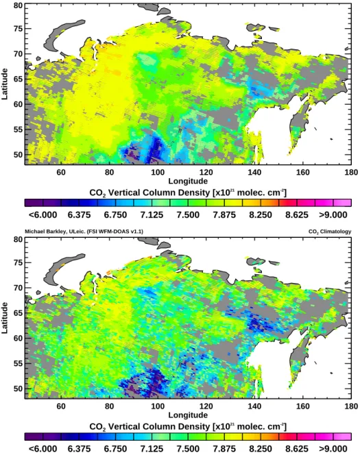
Fig. 10. Top panel: a priori CO2columns used in the retrieval for June, 2003, constructed from the CO2climatology. Bottom panel: The FSI WFM-DOAS retrieved CO2columns for the same month.

spectra and weighting functions. From close examination of the fit residuals, a Gaussian slit function of width 1.4 nm has been implemented as this yields the lowest retrieval er-rors and best fits. The root-mean-square (RMS) error, over the time-period considered, is extremely consistent at about 0.2% showing that the FSI algorithm is very stable (Table 4). Although the algorithm uses several sources of a priori in-formation it is important to ensure that the retrieved columns are not biased from the input data. This is especially

rele-vant with regards to the a priori CO2vertical columns, the

surface albedo and surface pressure. The a priori and

re-trieved CO2vertical columns for June (Fig. 10) demonstrate

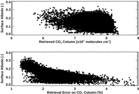
that whilst the spatial distribution of input columns is moder-ately smooth (essentially following the surface topography) the measured columns exhibit much more variation. The cor-relation between the two sets of columns, though relatively high at 0.82, is acceptable considering the low variability in the total column (Fig. 11). For the surface albedo no such correlation is found (Fig. 12), although the retrievals errors increase when the surface reflectance becomes progressively lower (i.e. as SCIAMACHYs signal to noise ratio decreases). Concerning the input ECMWF surface pressure, the corre-lation with the retrieved vertical column densities is again,

Fig. 11. The retrieved CO2columns as a function of the a priori CO2columns (shown in Fig. 10) for June 2003. The red line indicates a one-to-one relationship. The linear correlation coefficient between the data is 0.82.

5 6 7 8 9 Retrieved CO2 Column [x10 21 _{molecules cm}-2_] 0.0 0.1 0.2 0.3 0.4 Surface Albedo [-] 1 2 3 4 5

Retrieval Error on CO2 Column [%]

0.0 0.1 0.2 0.3 0.4 Surface Albedo [-]

Fig. 12. Top panel: The retrieved CO2columns, shown here for the month of May, haven’t any dependency on the a priori surface albedo. Bottom panel: The retrieval errors clearly increase when the a priori surface reflectance is small.

being well mixed in the atmosphere. If comparisons are made to the surface elevation (Fig. 13) however, which is on a finer resolution grid, then a slight bias is noticeable in that a significant fraction of the columns lie below the 3% (and indeed 5%) variability associated with the U.S. Stan-dard atmosphere. This in itself, is not indicative that retrieval algorithm produces this bias as it is possible that a large

num-ber of these low column densities may still be partially cloud contaminated. Alternatively, these low values may be a cali-bration related effect. The origin of this systematic underes-timation requires further examination. Checks for trends and biases in the retrieved CO2columns related to the

longitudi-nal and latitudilongitudi-nal distribution of the ground pixels, the line of sight and solar zenith angles and the a priori and retrieved

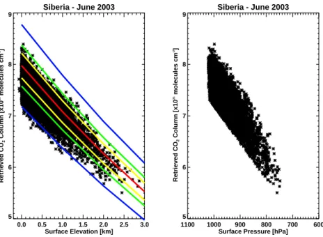
Siberia - June 2003 0.0 0.5 1.0 1.5 2.0 2.5 3.0 Surface Elevation [km] 5 6 7 8 9 Retrieved CO 2 Column [x10 21 molecules cm -2] Siberia - June 2003 1100 1000 900 800 700 600

Surface Pressure [hPa] 5 6 7 8 9 Retrieved CO 2 Column [x10 21 molecules cm -2]

Fig. 13. Left: Comparison between the surface elevation and the retrieved CO2columns. The surface elevation is taken from the GLOBE Digital Elevation Model (DEM) (http://www.ngdc.noaa.gov/mgg/topo/globe.html) and averaged to a 0.25◦×0.25◦grid. The linear corre-lation coefficient is −0.815. Over-plotted are the variations, of the vertical column density with surface elevation, for the U.S. Standard atmosphere (red), the U.S. Standard atmosphere ±3% variability in the total column (yellow), the U.S. Standard atmosphere ±5% variability (green) and the U.S. Standard atmosphere ±10% variability (blue). Right: The variation of the retrieved CO₂column with the a priori ECMWF surface pressure, which has a correlation coefficient of 0.82.

water vapour columns were also performed. In all circum-stances no correlation was found. This analysis was also

re-peated for the retrieval error associated with CO2 columns

with again, no biases detected.

Having considered the quality of the FSI retrieval algo-rithm, its results are shown in Fig. 14 with all normalized

columns averaged on to a 1◦×1◦grid. The most noticeable

feature of these monthly fields is the fairly high variability

of the CO2concentration, with the 1σ deviation about each

monthly mean being ∼10 ppmv. Whilst some of this vari-ability may be realistic it is probable that some of the

de-viations may be removed by normalizing the retrieved CO2

columns with oxygen (O2) columns, instead of the surface

pressure. By taking the ratio with oxygen, which can also be retrieved from SCIAMACHY, the effects of aerosols and clouds on the light path may cancel out. This so-called dry mixing ratio denoted XCO2(=CO2/O2×0.295) is used to

re-duce systematic errors in satellite retrievals and is already im-plemented by Buchwitz et al. (2005b) and proposed for the future Orbiting Carbon Observatory (OCO) mission (Crisp et al., 2004). However, fundamental differences between the radiative transfer and the averaging kernels of the respective

CO2 and O2 spectral fitting regions suggests that a proxy,

derived from an wavelength interval closer to the 1.57 µm

CO2 band, would be more beneficial. This not

withstand-ing, distinct evolving patterns within the CO2 distribution

are visible, for example there is an enhanced region over the

Yablononvyy mountain range (approximately 115◦E 49◦N)

in May and what seems to be a persistent dip in the CO2

concentration over the West Siberian Plain in the vicinity

of 75◦_{E 60}◦_{N. Similarly the seasonal uptake of CO}

2 by

the biosphere appears to be detectable with a decline in the concentration from May to July before increasing again by

September. Whether these features are created by CO2

sur-face fluxes is yet unproven and warrants further investigation. Nevertheless it is encouraging that some structure within the

CO2fields is visible and may possibly provide information

on important carbon processes occurring within the Siberian region. As more SCIAMACHY data is processed, the iden-tification of CO2surface fluxes will be the goal of future

re-search efforts.

6 Conclusions

The ability of the WFM-DOAS retrieval algorithm to

mea-sure total columns of atmospheric CO2has been closely

ex-amined. A detailed sensitivity analysis has been performed that has identified several non-negligible error sources and time dependent biases which affect the accuracy of the

re-trieved CO2columns. These inaccuracies originate from

us-ing a reference spectrum which is created from a differus-ing atmospheric state to that of the measurement. To minimize

60 80 100 120 140 160 180 Longitude 50 55 60 65 70 75 80 Latitude

CO2 Volume Mixing Ratio [ppmv]

<350.00 355.00 360.00 365.00 370.00 375.00 380.00 385.00 >390.00 SCIAMACHY/FSI CO2 - May 2003 60 80 100 120 140 160 180 Longitude 50 55 60 65 70 75 80 Latitude

CO2 Volume Mixing Ratio [ppmv]

<350.00 355.00 360.00 365.00 370.00 375.00 380.00 385.00 >390.00 SCIAMACHY/FSI CO2 - June 2003

60 80 100 120 140 160 180 Longitude 50 55 60 65 70 75 80 Latitude

CO2 Volume Mixing Ratio [ppmv]

<350.00 355.00 360.00 365.00 370.00 375.00 380.00 385.00 >390.00 SCIAMACHY/FSI CO2 - July 2003 60 80 100 120 140 160 180 Longitude 50 55 60 65 70 75 80 Latitude

CO2 Volume Mixing Ratio [ppmv]

<350.00 355.00 360.00 365.00 370.00 375.00 380.00 385.00 >390.00 SCIAMACHY/FSI CO2 - Sept 2003

Fig. 14. Normalized CO₂columns, retrieved over the Siberian test region for the summer of 2003, averaged on to a 1◦×1◦grid.

Initiation (FSI) WFM-DOAS has been developed, the foun-dation of which is the use of a priori data to obtain the best possible linearization point for the retrieval. The FSI algo-rithm has then been applied to SCIAMACHY observations with both the quality of the spectral fits and possible biases

assessed. Although some of the CO2columns appear to be

under-estimated there isn’t any evidence of a priori influence in the retrieved data. Preliminary results for the summer months over Siberia have shown that the retrieved monthly fields exhibit a significant amount of variability but that some structure in the CO2concentration is visible.

Acknowledgements. The authors would like to thank J. Burrows

and the team at IUP Bremen for providing such a useful instrument and for supplying preliminary SCIAMACHY data. Many thanks go to M. Buchwitz and C. Frankenberg for giving very helpful advice and comments. We are also grateful to M. Grzegorski for providing the HICRU cloud data and A. Rozanov for supplying the radiative transfer model SCIATRAN. We would like to thank ESA for supplying the SCIAMACHY data, all of which was processed by DLR, and the British Atmospheric Data Centre (BADC) for supplying the ECMWF operational data set. The authors finally wish to thank both the Natural Environment Research Council (NERC) and CASIX (the Centre for observation of Air-Sea Interactions and fluXes) for supporting M. Barkley through grant ref: NER/S/D/200311751.

Edited by: A. Hofzumahaus

References

Anderson, B. E., Gregory, G. L., Collins Jr., J. E., Sachse, G. W., Conway, T. J., and Whiting, G. P.: Airborne observations of spa-tial and temporal variability of tropospheric carbon dioxide, J. Geophys. Res., 101, 1985–1997, 1996.

Barkley, M. P., Monks, P. S., Frieß, U., Mittermeier, R. L., Fast, H., K¨orner, S., and Heimann, M.: Comparisons between SCIA-MACHY atmospheric CO2retrieved using (FSI) WFM-DOAS to ground based FTIR data and the TM3 chemistry transport model, Atmos. Chem. Phys. Discuss., 6, 5837–5425, 2006,

http://www.atmos-chem-phys-discuss.net/6/5837/2006/. Bovensmann, H., Burrows, J. P., Buchwitz, M., Frerick, J., N¨oel, S.,

Rozanov, V. V., Chance, K. V., and Goede, A.: SCIAMACHY – mission objectives and measurement modes, J. Atmos. Sci., 56, 127–150, 1999.

Buchwitz, M. and Burrows, J. P.: Retrieval of CH₄, CO, and CO₂ total column amounts from SCIAMACHY near-infrared nadir spectra: Retrieval algorithm and first results, in: Remote Sens-ing of Clouds and the Atmosphere VIII, ProceedSens-ings of SPIE, edited by: Sch¨afer, K. P., Com`eron, A., Carleer, M. R., and Pi-card, R. H., 5235, 375–388, 2004.

Buchwitz, M., Rozanov, V. V., and Burrows, J. P.: A near infrared optimized DOAS method for the fast global retrieval of atmo-spheric CH4, CO, CO2, H2O, and N2O total column amounts from SCIAMACHY/ENVISAT-1 nadir radiances, J. Geophys. Res., 105, 15 231–15 246, 2000.

Buchwitz, M., de Beek, R., Bramstedt, K., N¨oel, S., Bovensmann, H., and Burrows, J. P.: Global carbon monoxide as retrieved from SCIAMACHY by WFM-DOAS, Atmos. Chem. Phys., 4, 1945– 1960, 2004,

http://www.atmos-chem-phys.net/4/1945/2004/.

Buchwitz, M., de Beek, R., Burrows, J. P., Bovensmann, H., T.Warneke, Notholt, J., Meirink, J. F., Goede, A. P. H., Bergam-aschi, P., K¨orner, S., Heimann, M., and Schulz, A.: Atmospheric methane and carbon dioxide from SCIAMACHY satellite data: initial comparison with chemistry and transport models, Atmos. Chem. Phys., 5, 941-962, 2005a.

Buchwitz, M., de Beek, R., N¨oel, S., Burrows, J. P., Bovensmann, H., Bremer, H., Bergamaschi, P., K¨orner, S., and Heimann, M.: Carbon monoxide, methane and carbon dioxide columns re-trieved from SCIAMACHY by WFM-DOAS: year 2003 initial data set, Atmos. Chem. Phys., 5, 3313–3329, 2005b.

Ch´edin, A., Saunders, R., Hollingsworth, A., Scott, N. A., Ma-tricardi, M., Etcheto, J., Clerbaux, C., Armante, R., and Crevoisier, C.: The feasibility of monitoring CO₂ from high-resolution infrared sounders, J. Geophys. Res., 108, 4064, doi:10.1029/2001JD001443, 2003.

Ciais, P., Tans, P. P., Trollier, M., White, J. W., and Francey, R. J.: A large Northern Hemisphere terrestrial CO2sink indicated by the13C/12C ratio of atmospheric CO2, Science, 269, 1098–1101, 1995.

Conway, T. J., Tans, P. P., Waterman, L. S., Thoning, K. W., Kitzis, D. R., Masarie, K. A., and Zhang, N.: Evidence for interannual variability of the carbon cycle from the National Oceanic and Atmospheric Administration/Climate Monitoring and Diagnostic Laboratory Global Air Sampling, J. Geophys. Res., 99, 22 831– 22 855, 1994.

Crisp, D., Atlas, R., Br´eon, F.-M., Brown, L., Burrows, J., Ciais, P., Connor, B., Doney, S., Fung, I., Jacob, D., Miller, C., O’Brien, D., Pawson, S., Randerson, J., Rayner, P., Salawitch, R., Sander, S., Sen, B., Stephens, G., Tans, P., Toon, G., Wennberg, P., Wofsy, S., Yung, Y., Kuang, Z., Chudasama, B., Sprague, G., Wiess, B., Pollock, R., Kenyon, D., and Schroll, S.: The Orbit-ing Carbon Observatory (OCO) mission, Adv. Space Res., 34(4), 700–709, 2004.

de Beek, R., Gloudemans, A., Schrijver, H., Frankenberg, C., Grze-gorski, M., Wagner, T., and Buchwitz, M.: Retrieval algorithm development for EVERGREEN using SCIAMACHY: Status and analyses for optimization, Technical Note (EU Contract EVG1-CT-2002-00079),TN-EVG-TASK1-RET-001, 2004.

Dufour, E. and Br´eon, F.: Spaceborne estimate of atmospheric CO2 column by use of the differential absorption method: error anal-ysis, Appl. Opt., 42, 3595–3609, 2003.

Frankenberg, C., Platt, U., and Wagner, T.: Retrieval of CO from SCIAMACHY onboard ENVISAT: detection of strongly pol-luted areas and seasonal patterns in global CO abundances, At-mos. Chem. Phys., 5, 1639–1644, 2005a.

Frankenberg, C., Platt, U., and Wagner, T.: Iterative maximum a posteriori (IMAP)-DOAS for retrieval of strongly absorbing trace gases: Model studies for CH4and CO2retrieval from near infrared spectra of SCIAMACHY onboard ENVISAT, Atmos. Chem. Phys., 5, 9–22, 2005b.

GLOBALVIEW-CO2: Cooperative Atmospheric Data Integration Project – Carbon Dioxide, CD-ROM, NOAA CMDL, Boulder, Colorado [Also available on Internet via anonymous FTP to ftp:

//ftp.cmdl.noaa.gov, Path:ccg/co2/GLOBALVIEW], 2005. Gloudemans, A. M. S., Schrijver, H., Kleipool, Q., van den Broek,

M. M. P., Straume, A. G., Lichtenberg, G., van Hees, R., Aben, I., and Meirink, J. F.: The impact of SCIAMACHY near-infrared instrument calibration on CH4 and CO total columns, Atmos. Chem. Phys., 5, 2369–2383, 2005,

http://www.atmos-chem-phys.net/5/2369/2005/.

Grzegorski, M., Frankenberg, C., Platt, U., Sangahvi, S., Fournier, N., Stammes, P., and Wagner, T.: Application of the HICRU cloud algorithm on SCIAMACHY: design and intercomparision, Geophys. Res. Abstr., 7, 08316, 2005.

Gurney, K. R., Law, R. M., Denning, A. S., Rayner, P. J., Baker, D., Bousquet, P., Bruhwilerk, L., Chen, Y.-H., Ciais, P., Fan, S., Fung, I. Y., Gloor, M., Heimann, M., Higuchi, K., John, J., Maki, T., Maksyutov, S., Masariek, K., Peylin, P., Pratherkk, M., Pakkk, B. C., Randerson, J., Sarmiento, J., Taguchi, S., Taka-hashi, T., and Yuen, C.-W.: Towards robust regional estimates of sources and sinks using atmospheric transport models, Nature, 415, 626–630, 2002.

Heimann, M. and K¨orner, S.: The Global Atmospheric Tracer Model TM3, Model Description and Users Manual Release 3.8a, Tech. Rep. 5, Max Planck Institute for Biogeochemistry (MPI-BGC), Jena, Germany, 2003.

Hess, M., Koepke, P., and Schult, I.: Optical properties of aerosols and clouds: The software package OPAC, Bull. Am. Meteorol. Soc., 75, 831–844, 1998.

Holzer-Popp, T., Schroedter, M., and Gesell, G.: Retrieving aerosol optical depth and type in the boundary layer over land and ocean from simultaneous GOME spectrometer and ATSR-2 radiome-ter measurements, 1. Method description, J. Geophys. Res., 107, 4578, doi:10.1029/2001JD002 013, 2002.

Hoogen, R.: Aerosol Parameterization in GOMETRAN ++, In-stit¨ute fur Umweltphysik, Univ. of Bremen, Germany, Internal report, 1995.

Houweling, S., Hartmann, W., Aben, I., Schrijver, H., Skidmore, J., Roelofs, G.-J., and Br¨eon, F.-M.: Evidence of systematic errors in SCIAMACHY-observed CO2due to aerosols, Atmos. Chem. Phys., 5, 3003–3013, 2005,

http://www.atmos-chem-phys.net/5/3003/2005/.

Intergovernmental Panel on Climate Change: Climate Change 2001: Synthesis Report: Third Assessment Report of the Inter-governmental Panel on Climate Change, Cambridge University Press, New York, 2001.

Kawa, S. R., Erickson-III, D. J., Pawson, S., and Zhu, Z.: Global CO2transport simulations using meteorological data from the NASA data assimilation system, J. Geophys. Res., 109, D18312, doi:10.1029/2004JD004554, 2004.

Kleipool, Q.: Algorithm Specification for Dark Signal Determina-tion, Tech. rep., SRON-SCIA-30 PhE-RP-009, SRON, 2003a. Kleipool, Q.: Recalculation of OPTEC5 Non-Linearity, Report

con-taining the NL correction to be implemented in the data proces-sor, Tech. rep. SRON-SCIA-PhE-RP-013, SRON, 2003b. Kleipool, Q.: SCIAMACHY: Evolution of Dead and Bad Pixel

Mask, Tech. Report SRON-SCIA-PhE-RP-21, SRON, 2004. Kneizys, F. X., Shettle, E. P., Abreu, L. W., Chetwynd, J. H.,

An-derson, G. P., Gallery, W. O., Selby, J. E. A., and Clough, S. A.: A users guide to LOWTRAN 7, Tech. rep. Air Force Geophysics Laboratory AFGL, 1986.

Chetwynd, J. H., Shettle, E. P., Berk, A., Bernstein, L., Robert-son, D., Acharya, P., Rothman, L., Selby, J. E. A., Allery, W. O., and Clough, S. A.: The MODTRAN 2/3 report and LOWTRAN 7 model, Tech. rep., Philips Laboratory, Hanscom AFB, 1996. Kuang, Z., Margolis, J., Toon, G., Crisp, D., and Yung, Y.:

Space-borne measurements of atmospheric CO2by high-resolution NIR spectrometry of reflected sunlight: An introductory study, Geo-phys. Res. Lett., 29, 1716, doi:10.1029/2001GL014298, 2002. Kuck, L. R., Smith Jr., T. S., Balsley, B. B., Helmig, T.,

Con-way, T. J., Tans, P. P., Davis, K., Jensen, M. L., Bognar, J. A., Vazquez Arrieta, R., Rodriquez, R., and Birks, J. W.: Mea-surements of landscape fluxes of carbon dioxide in the Peruvian Amazon by vertical profiling through the atmospheric boundary layer, J. Geophys. Res., 105, 22 137–22 146, 2000.

Levin, I., Ciais, P., Langenfelds, R., Schmidt, M., Ramonet, M., Sidorov, K., Tchebakova, N., Gloor, M., Heimann, M., Schulze, E., Vygodskaya, N., Shibistova, O., and Lloyd, J.: Three years of trace gas observations over the EuroSiberian domain derived from aircraft sampling – a concerted action, Tellus, 54B, 696– 712, 2002.

Lichtenberg, G. , Kleipool, Q., Krijger, J. M., van Soest, G., van Hees, R., Tilstra, L. G., Acarreta, J. R., Aben, I., Ahlers, B., Bovensmann, H., Chance, K., Gloudemans, A. M. S., Hoogeveen, R. W. M., Jongma, R., Nol, S., Piters, A., Schri-jver, H., Schrijvers, C., Sioris, C. E., Skupin, J., Slijkhuis, S., Stammes, P., and Wuttke, M.: SCIAMACHY Level1 data: Cal-ibration concept and in-flight calCal-ibration, Atmos. Chem. Phys. Discuss., 5, 8925–8977, 2005,

http://www.atmos-chem-phys-discuss.net/5/8925/2005/. Mao, J. and Kawa, S. R.: Sensitivity studies for space-based

mea-surement of atmospheric meamea-surement of atmospheric total col-umn carbon dioxide by reflected sunlight, Appl. Opt., 43, 914– 927, 2004.

Matsueda, H., Inoue, H. Y., and Ishii, M.: Aircraft observations of carbon dioxide at 8–13 km altitude over the western Pacififc from 1933 to 1999, Tellus, 54B, 1–21, 2002.

McClatchey, R. A., Fenn, R. W., Selby, J. E. A., Volz, F. E., and Garing, J. S.: Optical properties of the atmosphere, 3rd ed., Env-iron. Res. Pap. 411, AFCRL-72-0497, Air Force Cambridge Res. Lab., Bedford, Mass., 1972.

Nakazawa, T., Miyashita, K., Aoki, S., and Tanaka, M.: Tempo-ral and spatial variations of upper tropospheric and lower strato-spheric carbon dioxide, Tellus, 43B, 106–117, 1991.

Nakazawa, T., Murayama, S., Miyashita, K., Aoki, S., and Tanaka, M.: Longitudinally different variations of lower tropospheric car-bon dioxide concentrations over the North Pacific Ocean, Tellus, 44B, 161–172, 1992.

Nakazawa, T., Sugawara, S., Inoue, G., Machida, T., Makshyutov, S., and Mukai, H.: Aircraft measurements of the concentrations of CO2, CH4, N2O and CO in the troposphere over Russia, J. Geophys. Res., 102, 3843–3859, 1997.

O’Brien, D. M. and Rayner, P. J.: Global observations of the car-bon budget, 2. CO₂column from differential absorption of re-flected sunlight in the 1.61µm band of CO2, J. Geophys. Res., 107(D18), 4354, doi:10.1029/2001JD000617, 2002.

Olsen, S. C. and Randerson, J. T.: Differences between sur-face and column atmospheric CO2 and implications for carbon cycle research, J. Geophys. Res., 109, D02 301, doi:10.1029/2003JD003968, 2004.

Rayner, P. J. and O’Brien, D. M.: The utility of remotely sensed CO2concetration data in surface source inversions, Geophys. Res. Lett., 28, 175–178, 2001.

Remedios, J. J., Parker, R. J., Panchal, M., Leigh, R. J., and Cor-lett, G.: Signatures of atmospheric and surface climate variables through analyses of infrared spectra (SATSCAN-IR), Proceed-ings of the first EPS/METOP RAO Workshop, ESRIN, 2006. R¨odenbeck, C., Houweling, S., Gloor, M., and Heimann, M.: CO₂

flux history 1982–2001 inferred from atmospheric data using a global inversion of atmospheric transport, Atmos. Chem. Phys., 3, 1919–1964, 2003,

http://www.atmos-chem-phys.net/3/1919/2003/.

Rothman, L., Jacquemart, D., Barbe, A., Benner, C. D., Birk, M., Brown, L. R., Carleer, M. R., Chackerian Jr., C., Chance, K., Coudert, L. H., Dana, V., Devi, V. M., Flaud, J.-M., Gamache, R. R., Goldman, A., Hartmann, J.-M., Jucks, J. W., Maki, A. G., Mandin, J.-Y., Massie, S. T., Orphal, J., Perrin, A., Rinsland, C. P., Smith, M., Tennyson, J., Tolchenov, R. N., Toth, R. A., Vander Auwera, J., Varanasi, P., and Wagner, G.: The HITRAN 2004 molecular spectroscopic database, J. Quant. Spectrosc. Ra-diat. Transfer, 96, 193–204, 2005.

Rozanov, V. V., Buchwitz, M., Eichmann, K. U., de Beek, R., and Burrows, J. P.: SCIATRAN – a new radiative transfer model for geophysical applications in the 240–2400 nm spectral region: The pseudo-spherical version, presented at COSPAR 2000, Adv. Space Res., 29(11), 1831–1835, 2002.

Sabine, C. L., Freely, R. A., Gruber, N., Key, R. M., Lee, K., Bullister, J. L., Wanninkhof, R., Wong, C. S., Wallace, D. W. R., Tilbrook, B., Millero, F. J., Peng, T.-H., Kozyr, A., Ono, T., and Roso, A. F.: The Oceanic Sink for Anthropogenic CO2, Science, 305, 367–371, 2004.

Schrijver H.: Retrieval of carbon monoxide, methane and nitrous oxide from Sciamachy measurements in: Proc. European Sym-posium on Atmospheric Measurements from Space, ESA WPP-161 1, ESTEC Noordwijk, The Netherlands, 285–294, 1999. Sidorov, K., Sogachev, A., Langend¨orfer, U., Lloyd, J.,

Nepomni-achii, I. L., Vygodskaya, N. N., Schmidt, M., and Levin, I.: Sea-sonal variability of greenhouse gases in the lower troposphere above the eastern European taiga (Syktyvkar, Russia), Tellus, 54B, 735–748, 2002.

Tans, P. P., Fung, I. Y., and Takahashi, T.: Observational constraints on the global atmospheric CO2 budget, Science, 247, 1431– 1438, 1990.

Vay, S., Anderson, B. E., Conway, T. J., Collins Jr., J. E., Blake, D. R., and Westberg, D. J.: Airborne observations of tropospheric CO2distribution and its controlling factors over the South Pacific Basin, J. Geophys. Res., 101, 1985–1997, 1999.

Yang, Z. H., Toon, G. C., Margolis, J. S., and Wennberg, P. O.: Ground based inversion of CO₂ column densi-ties from solar spectra, Geophys. Res. Lett., 29, 1339, doi:10.1029/2001GL014537, 2002.