HAL Id: hal-01396290
https://hal.sorbonne-universite.fr/hal-01396290
Submitted on 12 Mar 2020
HAL is a multi-disciplinary open access
archive for the deposit and dissemination of
sci-entific research documents, whether they are
pub-lished or not. The documents may come from
teaching and research institutions in France or
abroad, or from public or private research centers.
L’archive ouverte pluridisciplinaire HAL, est
destinée au dépôt et à la diffusion de documents
scientifiques de niveau recherche, publiés ou non,
émanant des établissements d’enseignement et de
recherche français ou étrangers, des laboratoires
publics ou privés.
Massimiliano Casaletti, Guido Valerio, Ronan Sauleau, Matteo Albani
To cite this version:
Massimiliano Casaletti, Guido Valerio, Ronan Sauleau, Matteo Albani. Mode-Matching Analysis of
Lossy SIW Devices. IEEE Transactions on Microwave Theory and Techniques, Institute of
Electri-cal and Electronics Engineers, 2016, 64 (12), pp.4126-4137. �10.1109/TMTT.2016.2605667�.
�hal-01396290�
Abstract— In this paper, the authors present a method for the analysis of lossy Substrate Integrated Waveguide (SIW) structures. The analysis is achieved through the cylindrical-wave mode expansion of the field and a mode matching technique to enforce boundary conditions on the post surfaces. We introduce an approximated formulation of the previous exact procedure, valid in the microwave regime, and numerically examine a number of microwave devices using both approximated and exact analyses. These devices include filters, couplers, phase shifter, etc. Results are presented for the scattering parameters and compared to those obtained with commercial software in terms of accuracy and computational time.
Index Terms— conductor losses, Green’s functions, method of moments (MoM), SIW
I. INTRODUCTION
ith an ever-increasing number of micro- and millimeter-wave devices being built in substrate-integrated waveguide (SIW) technology [1]-[4], and their inevitably increasing complexity (e.g., [5]-[7]), there is need for a fast and accurate method of analyzing and optimizing such devices. Moreover, with the shift of applications of this attractive technology to higher frequency bands (even as high as the D-band [8]), one needs to accurately assess conductor losses, which become the dominant loss mechanism in SIW-based devices at higher frequencies [9], significantly degrading the performance of devices, e.g., lowering the gain of slotted arrays or increasing the insertion loss of SIW-filters. This is especially important when low-cost fabrication techniques relying on low-conductivity metals are employed. In addition, the conductor roughness, especially of the ground plates, starts to play a role in the overall loss, further increasing it. This is particularly important for specific manufacturing technology as Low Temperature Co-fired Ceramic (LTCC) or low cost inkjet processes [10].
Over the past years, several methods for the analysis of SIW devices have been proposed, ranging from finite-difference schemes [11], equivalent-width waveguide methods [12],
Manuscript received 23/03/2015; revised DATE.
The authors would like to thank the Agence Nationale de la Recherche (grant ANR 2010 VERS 001301, grant ANR 12-EMMA-0041-01) and DGCIS (FUI 10, DENOTEIC).
M. Casaletti and G. Valerio are with the Sorbonne Universités, UPMC Univ. Paris 06, UR2, L2E, F-75005, Paris, France (e-mail: [email protected], [email protected]).
R. Sauleau is with the Institute of Electronics and Telecommunications of Rennes (IETR), UMR CNRS 6164, University of Rennes 1, 35042 Rennes, France (e-mail: [email protected]).
M. Albani is with the Dipartimento di Ingegneria dell’Informazione Università degli Studi di Siena, Via Roma 56, 53100, Siena, Italy (e-mail: [email protected]).
boundary integral-resonant method [13] and integral-equation-based methods [14]-[19]. However, most of these methods lack in generality, being applicable mostly to shielded PEC structures mimicking conventional rectangular waveguides [9], [17], [18], dealing with electrically thin cylindrical scatterers [14], or operating in the Transverse Magnetic (TM) mode regime [15]-[18]. This is a hindrance to designing, since one has to consider carefully the effect of all relevant modes [20]-[22], which may be induced at discontinuities in the system under consideration, and, more importantly, since the geometry may in general be irregular and quite complex. Furthermore, the losses were modeled using approximations of severely restricted validity, mostly by effective or empirically determined surface impedances as in [9] and [12]. In [16], losses were incorporated into an approximate mode-matching analysis of single-waveguide SIW structures. However, only the basic coaxial feed was used to excite the structures under study, limiting the analysis to the study of TM modes only. Moreover, the coaxial feeds were approximately modeled as magnetic currents radiating into an infinite perfectly electric conductor (PEC) parallel-plate waveguide (PPW). This may be valid when the conductivity of the ground plane is high, but when this is not the case, this approximation yields inaccurate feeding fields as the coaxial feed may induce higher-order modes in the waveguide. Also, the connecting vias were considered to be exclusively PEC, thus avoiding coupling between Transverse Electric (TE) and TM modes, which can be significant when low-conductivity metal is used.
Therefore, one needs a general, reliable and efficient analysis tool that could take into account properly the aforementioned effects and consequently be used in design and optimization. The authors have recently proposed a hybrid Method of Moments (MoM)/Mode-Matching (MM) method [21],[23], capable of accurately analyzing stacked planar SIW structures with the possible presence of coupling or radiating slots etched in conducting plates. Here we extend the
mode-matching part, which can be subsequently used as the building
block in the MoM framework (e.g., [23]), to incorporate conductor losses in a rigorous manner. The resulting code provides a reliable full-wave tool to design and optimize SIW devices by rigorously taking into account losses. A significant reduction of computation time and memory usage is achieved with respect to commercial software, especially when large structures are considered and need to be optimized.
The formulation of the problem in terms of lossy eigenfunctions is similar to the one presented in [24], where only slots in a PPW are considered in the absence of vertical posts. The formulation has been described with no mathematical details and no results in [25]. The need of
non-Mode-Matching Analysis of Lossy SIW Devices
Massimiliano Casaletti, Member, IEEE, Guido Valerio, Member, IEEE,
Ronan Sauleau, Senior Member, IEEE, and Matteo Albani, Senior Member, IEEE
orthogonal vertical eigenfunctions in the presence of lossy plates has been introduced in [26], together with preliminary numerical results of a structure not shown in this paper. However, details on the actual implementation are discussed here for the first time.
To be more specific, we model both the conductor losses and small metal surface roughness using the Leontovich boundary condition [27], granting the description of lossy or rough metal surfaces as surface impedances. This allows one to derive analytically the necessary scalar Green’s functions, and, subsequently, a set of scalar potentials from which the PPW dyadic admittance Green’s function can be obtained through differentiation [28]. The lossy metal vias are modeled either as lossy-dielectric cylinders, or as surface impedances, whose scattered fields can be found by enforcement of the impedance boundary conditions on their respective surfaces. In addition, we consider the effect of placing a coaxial feed over a lossy plane through the application of the equivalence principle in a rigorous manner.
The paper is organized as follows. Section II gives a brief outline of the derivation of both the necessary Green’s functions and the vector wave functions with special emphasis on the underlying mathematical structure.
In Section III, mode coupling in lossy SIW is quantitatively studied, while in Section IV an approximated mode-matching approach is derived, based on previous section results. Section V deals with the definition and computation of input parameters. Finally, in Section VI, we validate the results of numerical analysis by comparison against an FEM-based commercial code in terms of accuracy and computation time.
II. MATHEMATICAL BACKGROUND
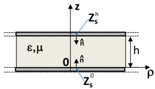
Fig. 1. Lateral view of a lossy PPW
In typical microwave applications, SIW channels are obtained by drilling commercial metalized dielectric substrates, and then filling the holes with conducting materials (or dielectric) in order to implement the cylindrical posts. This procedure leads to structures that use the same kind of metallization for both top and bottom planes. Moreover, at this frequency regime, the roughness of the metallization can be in general neglected. All these considerations lead to the use of the Leontovich equivalent boundary condition for the metallic planes
(
1)
/ 2( )
s s
Z = + j ωµ σ (1)
where
σ
is the conductivity,ω
is the angular velocity ands
µ
is the permeability. Other type of surfaces (such as thin metals [29], rough surfaces [30][31] or partially reflecting surfaces [32]) can be modeled through an equivalent impedance. For the sake of brevity, in this work only lossy metal plates will be considered henceforth.The structure under analysis consists of a PPW, defined by two horizontal lossy metallic plates placed at a distance h, laterally unbounded, filled by a dielectric medium (see Fig. 1). Inside the PPW an arbitrary number of vertical cylindrical posts can be placed, either of penetrable or impenetrable medium.
From a computational point of view, it is of paramount importance to choose the most effective representation according to the kind of field. In this view, the cylindrical eigenmode expansion of the field seems to be the appropriate choice [33]. The fields scattered by these posts can be modeled by linear sums of vector modes with unknown amplitude, while the incident field on the posts can be computed through a Green’s function represented in terms of eigenfunctions expansion [33]. The scattered amplitudes are then found by imposing boundary conditions on the post surfaces.
Vector functions are defined as in [30, Sec. 7.2]
( )
( )
( )
( )
ˆ , 1 ˆ , TM TE k = ∇ Φ = ∇ ∇ Φ M r z r N r z r × × × (2)referring to the transverse (with respect to z) magnetic field TMz and TEz polarization, respectively. The scalar Φ
functions must satisfy the scalar Helmholtz equation.
Assuming a
e
j tω time harmonic dependence, it can be solvedby conventional means, through separation of variables in cylindrical coordinates r≡
(
ρ φ
, , z)
(in anticipation of the presence of circular cylindrical scatterers), yielding( )
(
)
(
)
( )
(2) , m m t n t jn t mn m t m n J k c e z H k ρ φ ρρ
ρ
− Φ = ψ r (3)with t =TM/TE, where Jn and (2)
n
H are n-th order Bessel and second kind Hankel functions describing the radial dependence of fields inside and outside the posts, respectively.
m
t
k
ρ , mt z
k
are the m-th TM/TE mode transverse propagation constants and the z functions are eigenvalues of the Sturm-Liouville problem( )
( )
2 2 2 zt t 0 d k z dz + ψ = (4)subject to the following boundary conditions on the conductor plates
z
ρ
h
0
ε,µ
Z
shZ
s0 n n ^ ^(
)
( )
(
)
( )
0, 0, ˆ ˆ 0, ˆ ˆ 1 0. TM s z h TE s z h d j Z z dz Z d z j dz ωε ωµ = = − ⋅ ψ = − ⋅ ψ = n z n z (5)Since the coefficients of the terms in the boundary conditions are complex, this defines a nonself-adjoint Sturm-Liouville problem [30, Sec. 5.3]. If we wish to construct complete orthonormal sets based on these solutions in order to construct arbitrary fields, we need normalized eigenfunctions. This can be accomplished through a suitable choice of the coefficients
m
c . Using the L2-Hermitian inner product the eigenfunctions
ψ of the adjoint problem are obtained from a Helmholtz operator having a complex conjugate wavenumber and adjoint boundary conditions at the conducting plates.
Since the solutions ψ to the adjoint TM/TE problems are the complex conjugate of ψ , the normalization can be performed through the bi-orthogonality relationship as [22, Sec. 5.3]
( ) ( )
* 0 , h , t t t t m n m z n z dzδ
mn ψ ψ = ψ∫
ψ = (6)with t =TM/TE and
δ
mn denoting the Kronecker’s symbol1
mn
δ = when m n= or δ =mn 0 when m n≠ . This procedure leads to
(
)
(
)
( )
(
)
( )
( )
( )
( )
* 2 2 * 2 2 cos sin 2 , 2 sin cos 2 . 2 m m m m m m TM TM TM m z s z TM TM m m TM TM TM m s m s z TE TE TE m z s z TE TE m m TE TE TE m s m s z Z k z jZ k z h Z Z jZ Z k h Z k z jZ k z h Z Z jZ Z k h + ψ = ψ = − + − ψ = ψ = − − (7) where m , m TM TE m m TM z TE z Z k Z k ωµ ωε= = are the modal impedance of the
m-th TM/TE mode, respectively and TMm , TEm
z z
k k are the m-th solution (eigenvalues) of the following dispersion equations
(
)
(
)
(
)
( )
2 2 2 2 tan 2 0 tan 2 0 m m TM TM TM s m z m s TE TE TE s m z m s j Z Z k z Z Z j Z Z k z Z Z + + = + + = . (8)The field scattered by the posts in the whole SIW structure is thus expressed as a discrete sum of vector cylindrical waves defined as
( )
(
)
(
)
post 1 1 , , , , , , m m m m N TM TM TM s mnl n z l l m n TE TE TM mnl n z l A k k z A k k z ρ ρ +∞ +∞ = = =−∞ = − + − ∑ ∑ ∑
H r M ρ ρ N ρ ρ (9)where, for the vector eigenfunctions (2) the Bessel function
n
J is used for the field inside the posts, while the second kind Hankel function ( )2
n
H is used elsewhere.
Having obtained orthonormal bases for the eigenfunction expansion, we proceed to derive the dyadic magnetic Green’s function, given in [28],[24] as
(
)
(
)
( )
(
)
(
)
( )
(
) (
)
2 2 , 2 2 , 0 , 1 1 ˆˆ 1 , 4 1 , , , , , , 1 , , , , , , m m m m m m m m m m PPW HM t t t n TM TM TM TM m n z mn z TM m n n TE TE TE TE m n z mn z TE m n j k k k z k k z k k k z k k z k ρ ρ ρ ρ ρ ρ δ +∞ ∞ − = =−∞ +∞ ∞ − = =−∞ ∇ ∇ ′ = − + − ′ + × ∇ − ′ ′ − ′ ′ +∑ ∑
∑ ∑
G r r zz r r M ρ M ρ N ρ N ρ (10)Thus, the incident magnetic field radiated by a magnetic source JM distributed on a surface S′ is obtained as the
convolution of (10) with JM, resulting in
(
)
(
)
(
)
, 0 , 1 , , , , , , , m m m m PPW TM TM TM m n mn z m n TE TE TE m n mn z m n v k k z v k k z ρ ρ +∞ ∞ − = =−∞ +∞ ∞ − = =−∞ = ′ ′ ′ ′ ′ +∑ ∑
∑ ∑
H r r M ρ N ρ (11) where( )
( )
(
)
( )
0 2 2 ' 1 , , , , 4 m m m n r t t t t mn t mn z q M S v k k z d r kρ ρ ωε ε − ′ ′ ′ ′ = −∫
P ρ ρ− ⋅J r (12) with TM mn = mn P M , TE mn = mn P N .For a given source, the expansion coefficients for the field are found through a MM procedure by imposing boundary conditions on the post surfaces, as explained in next Section.
III. DETERMINATION OF THE COEFFICIENTS OF THE
SCATTERED FIELD EXPANSION
(a) (b)
Fig. 2. Vector eigenfunction expansion of the scattered field from: (a) impenetrable post; (b) penetrable post.
Once the dyadic Green’s function and vector wave functions are known, one can proceed to the formulation of the MM/MoM problem, since all types of fields (impressed and scattered) on the post surfaces can be described efficiently. A resolvable system of linear equations is obtained by imposing
xq yq q ρ q a ˆq n TM mnq A TE mnq A Zs ˆq n TM mnq A TE mnq A TM mnq B TE mnq B ( )q, ( )q ε µ q ρ
the appropriate boundary conditions.
A. Impenetrable posts
To determine the field scattered by an impenetrable post (Fig. 2a) of radius aq, described by a non-dispersive
impedance condition Zs, we impose the following boundary
condition on the surface of the post
( )
( )
TOT TOT ˆ ˆ ˆ q q q× ρ ρ− =′ a =Zs q× ×q ρ ρ− =′ a ρ E r ρ ρ H r (13)where ρˆq is the radial unit vector directed from the center of the post toward the exterior of the post, and ETOT and HTOT are
the total electric and magnetic fields, respectively. For Z =s 0
condition (13) resort to the PEC post case.
The fields are expanded through cylindrical wave functions as in (9). From the two scalar components of the vector identity (13) a couple of linear equations is obtained for the unknowns t
mnq
A . They are expressed as a series of azimuthal modes with linear phase around the q-th cylinder. From the orthogonality of the azimuthal eigenfunctions
e
jnφ (see [21])we can obtain two linear equations for each azimuthal harmonic
n
(
,)
n TM TE n
mnq mnq
f Aφ A =tφ , f Azn
(
mnqTM,ATEmnq)
=tzn (14)The two equations come from the φ and the z components of (13); fn
φ and fzn are linear functions of AmnqTM and AmnqTE , tφn
and n z
t are known quantities depending on the excitation current. For each harmonic
n
, (14) can then be projected on them
-th adjoint vertical eigenfunction tm
ψ
in order to obtain a linear system having the same number of equations and unknowns. The obtained equations contains the scalar products between different polarization eigenfunctions:, , ,
TE TM TM TE
m′ m m ′ m
ψ ψ ψ ψ .
If Z =s 0, (13) and (14) both reduce to the simpler case of a PEC post, where the TE and TM polarizations are decoupled.
B. Penetrable posts
Fig. 3. Incident scattered and transmitted field in a penetrable post.
To determine the field scattered from a penetrable (possibly lossy) post, whose radius is aq and complex dielectric
constants are ( )q , ( )q r r
ε
µ
, the continuity of the tangential electric and magnetic fields are imposed on the post surface (Fig. 3)ˆ PPW
( )
ˆ Posts( )
ˆ ( )( )
q q q q× + q× ρ ρ− =′ a = q× ρ ρ− =′ a ρ E r ρ E r ρ E r (15)( )
( )
( )( )
PPW Posts ˆ ˆ ˆ q q q q× + q× ρ ρ− =′ a = q× ρ ρ− =′ a ρ H r ρ H r ρ H r (16)where the superscripts ‘PPW’, ‘Posts’, and ‘q’ stand respectively for the fields excited in the PPW in the absence of the posts, for the fields scattered by all the posts, and for the field inside the q-th post under analysis. The fields in the waveguide are expanded through the Hankel function formulation of (9), while the field inside each cylinder is expanded through the Bessel function expression. Note that, if the post is metallic, a null field is retained inside the post, and only the electric field continuity (15) is used.
Each equation (15)-(16) can be projected along the
φ
and the z directions, thus obtaining a system of four scalar equations for the unknown coefficient TM TE/mnl
A and TM TE/
mnl
B .
These scalar equations are then projected on the basis of harmonic functions describing the azimuthal dependence of field around the considered cylinder. For each harmonic
n
, the two equations resulting from the components of (15) are(
,)
n TM TM n mnl mnl e A Bφ =tφ (17)(
, , ,)
n TM TE TM TE n z mnl mnl mnl mnl z e A A B B =t (18)and the two equations resulting from the components of (16) are
(
,)
n TE TE n mnl mnl h A Bφ =sφ (19)(
, , ,)
n TM TE TM TE n z mnl mnl mnl mnl z h A A B B =s (20)where e and h are linear functions of TM TE/
mnl
A and TM TE/
mnl
B , and t and s are known quantities depending on the excitation current. The four equations can then be projected on the vertical eigenfunctions
ψ
in order to obtain a linear system having the same number of equations and unknowns.Specifically, a careful choice of the eigenfunctions should be done in order to obtain stable solutions even for large losses in the cylinder. In fact, we can have eigenfunctions defined
inside the q-th post (where wavenumbers are referred to the
post dielectric), namely ( )q m
ψ , and eigenvalues defined in the PPW (where wavenumbers are referred to the PPW dielectric), namely ψm. It turns out that the best strategy is to project (17) and (19) on ψm, and (18) and (19) on ( )q
m ψ
(
,)
, 1 , 1 n TM TM TM n TM mnl mnl m m e A Bφ ψ = tφ ψ (21) xq yq q ρ q a ˆq n EPosts,HPosts ( )q, ( )q E H PPW PPW E H EM Source(
,)
, 2 , 2 n TE TE TE n TE mnl mnl m m h A Bφ ψ = sφ ψ (22)(
)
( ) ( ) 2 2 , , , , TE q TE q n TM TE TM TE n z mnl mnl mnl mnl m z m e A A B B ψ = t ,ψ (23)(
)
( ) ( ) 1 1 , , , , TM q , TM q n TM TE TM TE n z mnl mnl mnl mnl m z m h A A B B ψ = s ψ (24)We can derive explicit expressions for TM mnl
B from (21) and for TE
mnl
B from (22), and substitute them into (23) and(24). Using the bi-orthogonality relationship (6) we finally obtain two scalar equations for the unknowns TM
mnl
A and TE mnl
A . It turns out that with the above-mentioned testing choice, these expressions are composed only by terms having ratio of Bessel/Hankel functions of eigenvalue of the same medium. Thus, also with a large imaginary part of the argument the terms remain numerically stables.
In order to enforce (21)-(24), the computation of the following scalar products is required
( ) ( ) ( ) ( ) 1 2 1 2 1 2 , , , , , , , , , , , TM q TE TM TM TE TM m m m m w m TE q TE q TM q TE TM TE w m w m w m ′ ′ ψ ψ ψ ψ ψ ,ψ ′ ′ ψ ψ ψ ψ ψ ψ (25)
where ψmis the m-th TM or TE vertical eigenfunction in the
dielectric substrate, while ( )q m
ψ is the eigenfunction relative to the q-th dielectric post.
IV. APPROXIMATED MMFORMULATION
In this section we use an approximation of (25) in order to simplify the MM procedure developed in the previous section. Starting form analytical expressions (7), these products can be calculated rigorously in closed form and approximated as a series expansion for good conductive PPW walls.
In standard microwave applications, good conductors are characterized by small values of the ratioR ηs , where
( )
2s s
R =
ωµ
σ
and η= µ ε . Under this hypothesis, the wavenumbers solution of (8) can be approximated as in [24](
)
(
)
(
)
0 3 1 4 2 3 4 3 4 2 2 2 = 2 2 1,2, 2 = 2 1,2, m n j TM z s j TM z s j TE z s k R e h k m h R e m m n k n h R e n h π π π η ω εµ ω π η εµ π π π η εµ ω = + = … + = (26)Using (26) in the inner products (25) asymptotic expressions can be obtained for the coupling between different PPW modes for small values of R ηs .
(
)
(
)
(
)
(
)
( )(
)
(
)
( )(
)
(
)
2 , , 2 , , 2 , , 2 , , , , TM TE TM TE m n s m n s TE TM TM TE n m s m n s TM q TM TM TM m n s m n s TE q TE TE TE m n s m n mn mn mn mn s R O R R O R R O R R O R α η η α η η α η η α η δ δ δ δ η ′ ′ ψ ψ = + ∆ + ′ ′ ψ ψ = − + ∆ + ψ ,ψ = + ∆ + = ψ ,ψ + ∆ + (27)where α = 2 /µ εej34π and the amplitudes
,
m n
∆
depend on physical and geometrical parameters as shown in the appendix. For microwave applications the scalar products (25) can be safely approximated by the first terms of (27). In other words, (27) states that for typical microwave applications the scalar wavefunctions tm
ψ
of lossy SIW have the same properties as for the case of a lossless SIW. This means that the wave-vectors defined by (7) are quasi-orthogonal.A. Impenetrable posts
The field scattered by an impenetrable post of radius aq,
described by a non-dispersive impedance condition Zs under
the assumption (27) has to verify on the surface the following conditions for every couple of indexes
(
m n,)
(
)
( )(
)
( ) ( )(
)
(
)
(
)
( )(
)
( ) ( ) 2 2 -1, 2 2 1, 2 post lq m m m q m m m m m m post lq m m N j n n TM TM TM TM z r q mnl n n q l l l n TM TM TM mnq z n q TE TE TE TE q n q n q N j n n TE TE mnl n n q l l l q n TE TE mnq q n nk J k a A H k a e nA k H k a a jkk J k a k J k a A H k e A a jkk H k φ ρ ρ ρ ρ ρ ρ ρ φ ρ ρ ρ ϑ +∞ − − = ≠ =−∞ +∞ − − − = ≠ =−∞ + ′ + + × − ′ +∑ ∑
∑ ∑
ρ ρ(
)
( )(
)
(
)
(
)
(
)
2 2 2 , , m m m m m m m m m TE TE TE q n q TE TE TE TE TE m n q n q n q TM TM TM m n z n q a k H k a v a k J k a jkk J k a nv k J k a ρ ρ ρ ρ ρ ρ ρ ϑ ϑ − − + ′ = − − − (28)(
)
(
)
( )(
)
( ) ( )(
)
( )(
)
(
)
( )(
)
( ) 2 2 2 1, 2 2 2 1 m m m m post lq m m m m m lq m m m TM TM TM TM q n q n q N j n n TM TM mnl n n q l l l q n TM TM TM TM TM mnq q n q n q j n n TE TE TE TE z n q mnl n n q l l n a jk J k a kk J k a A H k e A a jk H k a kk H k a jnk J k a A H k e ρ ρ ρ ρ φ ρ ρ ρ ρ ρ φ ρ ρ ϑ ϑ ϑ +∞ − − − = ≠ =−∞ +∞ − − − = =−∞ − + ′ × − ′ + − + + −∑ ∑
∑
ρ ρ ρ ρ ( )(
)
(
)
(
)
(
)
1 1 1 2 1 1 1 1 1 1 1 , 2 , , post m m m m m m m m N l q TE TE TE m nq z n q TM TM TM TM TM m n q n q n q TE TE TE m n z n q jnA k H k a v a kk J k a jk J k a jnv k J k a ρ ρ ρ ρ ρ ρ ϑ ϑ ϑ ≠ − − + ′ = − + −∑
(29)where ϑ=Zs ζ , and ζ = µ µ ε ε0 r 0 r .
Eqs.(28)-(29) are valid also for PEC posts (ZS = =ϑ 0). In this particular situation, (28)-(29) reduce to
(
)
( )(
)
( ) ( )(
)
(
)
2 1, 2 , post lq m m m m N j n n TE TE TE n q mnl n n q l l l q n TE TE TE TE mnq n q m n n q J k a A H k e A H k a v J k a φ ρ ρ ρ ρ +∞ − − − = ≠ =−∞ − ′ − ′ ′ + = −∑ ∑
ρ ρ (30)(
)
( )(
)
( ) ( )(
)
(
)
1 1 2 1, 2 , post lq m m m m N j n n TM TM TM n q mnl n n q l l l q n TM TM TM TM mnq n q m n n q J k a A H k e A H k a v J k a φ ρ ρ ρ ρ +∞ − − − = ≠ =−∞ − − + = −∑ ∑
ρ ρ (31) B. Penetrable postsThe field scattered by a penetrable (possibly lossy) post, whose radius is aq and complex dielectric and magnetic
constants are ( )q , ( )q
r r
ε
µ
, have to grant the continuity of the total tangential electric and magnetic fields. These latter conditions, together with (27), lead to the following equations( )
(
)
(
( ))
( ) ( )(
)
(
( ))
(
)
( )(
)
( )(
)
( ) ( ) ( )(
)
(
( ))
( ) 2 2 2 2 2 2 2 2 2 2 2 2 2 2 2 2 2 2 1, 2 m m m m m m m m post lq m m m m m TE q TE TE TE q n q r n q n q TE q TE TE q TE r n q n q n q N j n n TE TE m nl n n q l l l q n q TE TE q TE r n q n q TE m nq TE q r J k a k J k a J k a k H k a J k a H k a A H k e k H k a J k a A k H ρ ρ ρ ρ ρ ρ ρ ρ φ ρ ρ ρ ρ ρ µ µ µ µ +∞ − − − = ≠ =−∞ ′ ′ − ′ ′ × − ′ +∑ ∑
ρ ρ ( )(
)
(
( ))
( ) ( ) ( ) ( )(
)
( )(
)
( )(
)
( ) ( ) 2 2 2 2 1 1 1 1 1 2 2 1 1 2 1 1 1 1 1 2 2 2 1, 2 1 1 m m m m m m m m m m m m post lq m m TE q TE n q n q TM TM q TM q TM TM n q z z TM q TM TM q TE TE q z n q N j n n TM TM m nl n n q l l l q n n TM m nq q k a J k a J k a k k k k jn ka k k k k H k a A H k e H k jn A ka ρ ρ ρ ρ ρ ρ ρ ρ ρ φ ρ ρ +∞ − − − = ≠ =−∞ − ′ + − ′ × − +∑ ∑
ρ ρ(
)
( ) ( )(
)
( ) ( ) ( ) ( )(
)
(
( ))
( ) ( )(
)
(
( ))
(
)
( )(
)
2 2 1 1 1 1 2 2 1 1 1 1 2 2 2 2 2 2 2 2 2 2 2 , 2 2 , 1 m m m m m m m m m m m m m m m m m TM q TM TM TM TM q q z z TM q TM TM q TE TE z n q q TE TE TE q TE r n q n q n q TE m n TE q TE TE q TE r n q n q n q TM m n a k k k k k k H k a k k k J k a J k a J k a v k H k a J k a H k a jn v k ρ ρ ρ ρ ρ ρ ρ ρ ρ ρ ρ ρ ρ ρ µ µ − − − ′ ′ ′ = − − ′ ′ − ( ) ( ) ( ) ( )(
)
( )(
)
2 2 1 1 1 1 1 2 2 1 1 1 1 1 2 1 m m m m m m m m m m TM TM q TM q TM TM n q z z TM q TM TM q TE TE q z n q J k a k k k k a k k k k H k a ρ ρ ρ ρ ρ ρ ρ − ′ (32)(
)
( )(
)
( )(
)
(
( ))
( ) ( )(
)
(
( ))
( )(
)
( ) ( ) ( )(
)
(
( ))
( ) 1 1 1 1 1 1 1 1 1 1 1 1 1 1 2 2 2 1, 2 1 m m m m m m m m post lq m m m m m q TM q TM TM TM n q r n q n q TM q TM q TM TM n q r n q n q N j n n TM TM mnl n n q l l l q n q TM TM TM q r n q n q TM m nq TM q r J k a k J k a J k a H k a k H k a J k a A H k e k H k a J k a A k ρ ρ ρ ρ ρ ρ ρ ρ φ ρ ρ ρ ρ ρ ε ε ε ε +∞ − − − = ≠ =−∞ ′ ′ − ′ ′ × − ′ + −∑ ∑
ρ ρ ( )(
)
(
( ))
( ) ( )(
)
( )(
)
( )(
)
( ) 1 1 2 2 2 2 1 2 1 2 2 1 2 2 2 2 2 1 1 2 2 2 1, 1 1 m m m m m m m m m m post lq m m m m TM q TM n q n q TE TE q TE TE n q z z TM TE q TE TM q z n q N j n n TE TE m nl n n q l l l q n TE TE z z TE m nq TM q H k a J k a J k a k k k jn ka k k k H k a A H k e k k k jn A ka k ρ ρ ρ ρ ρ ρ ρ φ ρ ρ ρ +∞ − − − = ≠ =−∞ ′ + − ′ × − + −∑ ∑
ρ ρ ( ) ( ) ( )(
)
( )(
)
(
)
( )(
)
( )(
)
(
( ))
( ) ( )(
)
(
( ))
( ) 2 2 2 1 2 2 1 1 1 1 1 1 1 1 1 2 2 2 1 1 2 2 , 2 2 , 1 m m m m m m m m m m m m m m m m m TE TE q n q TE q TE TM n q z q TM q TM TM TM n q r n q n q TM m n TM TM q TM TM q n q r n q n q TE q TE TE z z TE m n TM q H k a H k a k k J k a k J k a J k a v H k a k H k a J k a k k k jn v ka k k ρ ρ ρ ρ ρ ρ ρ ρ ρ ρ ρ ρ ρ ρ ε ε − − ′ ′ ′ = − − ′ ′ − − ( )(
)
( )(
)
2 2 1 2 2 2 m m m m TE n q TE q TE TM n q z J k a H k a k ρ ρ ′ (33)C. Determination of the expansion coefficients
Let the structure under analysis be composed by
N
posts. In order to numerically solve the equations (28)-(32), the number of retained azimuthally and vertical modesN
φ andz
N , respectively, can be chosen according to [21],[23]. Since vertical modes with different orders m are decoupled, it is possible to cast (28)-(32) for each value m= 1, ,Nz into the following matrix form
, , , , TM TM TM TE TM TM TE m m m m TE TM TE TE TE m m m + = T T A Ω T T A (34)
where Tm are the post interaction coupling matrices,
,
TTM TE m m
A A
is the unknown vector containing all the cylindrical waves coefficients and TM TE/m
Ω
is the excitation vector. The unknown field coefficients are then found by solving a Nzmatrix equations (33).V. INPUT PARAMETERS
In this Section we discuss the definition of excitation ports and the calculation of the input parameters, starting from the results obtained from the procedure described in the previous sections. Source modeling for specific geometries have been proposed in the past as in [21][34]. Here we follow the
formulation in [21]. We only outline the differences with the PEC walls case for a waveguide port excitation and a general excitation defined over the impedance walls (coaxial excitation, slots).
A. Waveguide Ports: Computation of the Input Parameters
The computation of the input parameters is performed according to the same approach presented in [21]. Once the j-th input port is fed wij-th j-the equivalent magnetic current hj, a
modal decomposition is performed on the total magnetic field
Hi at the i-th port for each i, by projecting Hi on the
rectangular waveguide modes hnm (the TE10 fundamental mode
is used in the following, being usually sufficient for our scopes). The field Hi can be decomposed in a field
(
)
01( )
PPW , TE
q j ⋅ j j
G r r h r excited in the absence of posts (i.e., computed through the PPW Green’s function) and a field
HPosts scattered by posts (determined through the mode
matching)
( )
(
)
( )
( )
( )
01 01 01 PPW TE TE TE Posts PPW Posts , q j q q q j qj w w q q q j j j j q P P P w q q q q P Y j Z Z dS dS Z dS Y Y ωε = ⋅ ⋅ ⋅ + ⋅ = +∫ ∫
∫
h r G r r h r h r H r (35)The computation of YPPW can be performed by moving on
the current h the derivatives present in the definition of the
Green’s function. The details are shown in [21], while an efficient computation of YPosts has been presented in [23].
However, the presence of impedance boundary condition on the PPW plates leads to a different integral expression for
YPPW. In fact in this new structure, since the TM and TE radial
wavenumbers are different, the z-derivative of the scalar potential
S
TE does not cancel out the scalar potentialS
TM.Following [24], after a lengthy calculation, the final expression for YPPW is
(
)
(
)
(
)
(
)
( )
(
)
( )
01 01 01 01 TE TE 2 TM 2 TE TE TE TE 2 TM , , , ˆ ˆ , q j q j q j PPW w w qj u q u j P P q j w w q j q q j j P P Z Z Y h h k S j k S G dS dS Z Z k h G h dS dS j ωµ ωµ ′ ′ = − ∂ ∂ − ′ ′ ′ + − ′ ′ − ⋅∫ ∫
∫ ∫
r r r r r r u u r r r r (36)where
G
TEis a dual TE Green’s function (appearing in [24] in connection with slot modeling). It corresponds to the current in a TE equivalent transmission line fed by a unit series voltage generator, as opposed to the conventional GTE Green’sfunction (a voltage in a TE equivalent transmission line fed by a unit shunt current generator) [28].
B. Coaxial Cables and slots: Computation of the Admittance Matrix
Coaxial cables can be described through equivalent currents placed on one of the PPW plates [21], as shown in Fig. 4a. However, due to the presence of losses, the equivalent input and output magnetic currents are not placed on PEC plates (i.e., short circuits), as required by the definition of the admittance matrix. In order to keep the formulation simpler and similar to that one of PEC case, only the magnetic currents defined over the uniform impedance wall are used as source (Fig. 4b). In a SIW system excited by N coaxial ports (with inner radius aj and outer radius bj), this particular
feeding choice leads to the equivalent network illustrated in Fig. 4c, where further impedances
(
)
1 ln 1 ln 1 1 2 2 2 j j j L j j b b Z j a a µ ωµ π ε π σ = = + (37)are connected to the input ports.
For this reason, once the output currents at each port are determined for each feeding configuration, we need to perform a post processing ready to compute the correct admittance matrix
Y
of the structure.Let us feed the i-th port with a voltage Vi, as shown in Fig.
4c. The procedure proposed in [21] allows computing the output current on the j-th port i
j
I . The ratio i /
j i
I V is the ij element of the matrix YL. On the other hand, the entries of
the admittance matrix
Y
are defined with respect to the voltages ˆii
V at the input of the N-port network, i.e., after each impedance ZL.
(a) (b)
(c)
Fig. 4. (a) Coaxial excitation’s equivalent electric and magnetic currents. (b) Magnetic sources defined over the impedance condition used in the mode-matching technique. (c) Equivalent Y model of the SIW device under analysis. s Z Meq eq J s Z eq M s Z i V j L Z i i I i j I 1 v 1i I i N I … … … … i L Z N L Z 1 L Z
Y
ˆi i V 1 ˆi V ˆi N V ˆi j VWe can write
ˆi = − L i+ i
V Z I V (38)
where we have defined the column vectors
1 1 ˆ 0 ˆ ˆ , , 0 ˆ i i i i i i i i i i i i N N V I V I V I V = = = V I V (39)
and the diagonal matrix
1 0 0 L L N L Z Z = Z . (40)
Since for every i
ˆ
i= ⋅ i
I Y V (41)
we can replace (38) into (41)
L
i = − ⋅ + ⋅i i
I Z Y I Y V (42)
Once N different simulations are performed, one for each excitation, we can define the following matrices
(
1 N)
,(
1 N)
= =
I I I V V V (43)
and the following relation holds
(
)
(
)
1L L
−
= ⋅ − ⇒ = ⋅ −
I Y V Z I Y I V Z I (44) By replacing in (44) the simulated results
I Y V
=
L⋅
, wefinally obtain a simple expression for the admittance matrix Y
(
)
1L L
−
= ⋅ ⋅ − ⋅
Y Y V V Z V (45)
If the same excitation is assumed for all the ports,
V
=
V
1
(1being the identity matrix) and
(
)
1 L L L − = ⋅ − Y Y 1 Z Y (46)An equivalent of the above mentioned procedure could be obtained in terms of equivalent currents, by using the results in [24]. A slot excitation can be described only with equivalent magnetic currents allowing the use of the procedure presented in [23] to study multi-waveguide SIW systems.
VI. NUMERICAL RESULTS
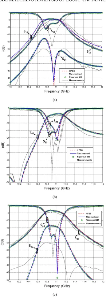
In this section we apply the rigorous and approximated proposed methods for the analysis of SIW microwave devices available in the scientific literature. Four examples have been selected in order to test different features of the method. All the results have been compared with numerical simulation performed with the finite elements commercial software Ansys HFSSTM 15. For the reader’s convenience the measured
parameters taken from the original articles are also included. The first example is a frequency-selective power combiner/divider [35]. The structure and the relevant geometrical parameters are given in Fig. 5. The structure is
composed by 108 copper posts and is fed by four waveguide ports, each one modeled through an array of PEC posts [21]. The S-parameters of the structures computed with the rigorous and approximated methods are compared to HFSSTM
simulations in Fig. 6. A very good agreement is found among all these methods and the measurements performed in [21]. The second example is the SIW right-angle corner proposed in [36]. It consists of 32 copper posts in a corner arrangement and 273 air posts working as an integrated lens. The transition is fed by 2 ports. The top view of the structure is shown in Fig. 7. The interest of this test case is the presence of a large number of dielectric posts. Fig. 8 compares the calculated scattering parameters. A very good agreement is obtained between the simulated transmission parameters S12. Small
differences in the reflection parameter S11 are due to the very
low level of this parameter.
The third example is a linear phase filter [37] composed by 80 copper posts and 4 rectangular slots acting as reactive loads. The complete structure is shown in
Fig. 9. The slots are modeled according to the method of moments approach described in [24] by using 5 entire domain basis functions for each slot. The slots admittances are modified according to Section V to rigorously take into account losses. The relevant results are plotted in Fig. 10.
The last example is a large system implementing a generalized Chebychev diplexer [38], composed by 414 copper posts and fed by 3 ports shown in Fig. 11. Also for this last case (see Fig. 12), a very good agreement between scattering parameters is obtained.
We report in Tables I and II the CPU time and used memory for the considered cases and compare them to those of HFSSTM. The data have been generated using a Personal
Computer with a 2.8 GHz Intel I7 870 CPU, while the proposed methods have been implemented in MatlabTM. The
actual implementation of the codes does not take advantage of multi-core or multi-CPU systems, but it can be parallelized.
Fig. 5. Geometry of the frequency-selective power combiner/divider [35]. Physical parameters of the substrate: height h = 0.508 mm, relative permittivity εr=2.33, loss tangent tanδ = 0.0012. All dimensions are expressed
(a)
(b)
(c)
Fig. 6. Comparison of the magnitude of the scattering parameters for the test structure represented in Fig. 5: this method (blue solid lines), rigorous method (green circles), HFSSTM (red dashed lines) and measurements (black dotted
lines). (a) S1X parameters, (b) S2X parameters, (c) S3X parameters. Measurements taken from [21].
Fig. 7. SIW right-angle corner [36]. Physical parameters of the substrate: height h = 0.508 mm, relative permittivity εr = 4.5, loss tangent tanδ = 0.002.
All dimensions are expressed in millimeters.
Fig. 8. Comparison of the magnitude of the scattering parameters for the structure represented in Fig. 7: this method (blue solid lines), rigorous method (green circles), HFSSTM (red dashed lines) and measurements (black dotted
lines). Measurements taken from [36].
Fig. 9. Geometry of the linear phase filter in quadruplet topology with frequency-dependent couplings [37]. Physical parameters of the substrate: height h=0.762, relative permittivity εr=3.46, loss tangent tanδ=0.0018. All
dimensions are expressed in millimeters.
These results demonstrate that the proposed algorithm is extremely efficient both in terms of computational and memory requirements. Moreover, since it does not need any meshing, it can play a key-role in design optimization procedures where geometrical parameters are changed.
3.26 2.36 0. 91 0.5 1 6. 37 0. 27 0. 2 Port 1 Port 2
Fig. 10. Comparison of the magnitude of the scattering parameters for the structure represented in Fig. 9: this method (blue solid lines), rigorous method (green circles), HFSSTM (red dashed lines) and measurements (black dotted
lines). Measurements taken from [37].
Fig. 11. Geometry of the generalized Chebyshev SIW diplexer [38]. Physical parameters of the substrate: height h= 0.762 mm, relative permittivity εr=3.46,
loss tangent tanδ = 0.0018. All dimensions are expressed in millimeters.
Fig. 12. Comparison of the magnitude of the scattering parameters for the structure represented in Fig. 11. This method (blue solid lines), rigorous method (green circles), HFSSTM (red dashed lines) and measurements (black
dotted lines). Measurements taken from [38].
TABLE I
CPU SIMULATION TIME ON A XEON E55402.83GHZ WITH 16GBYTE RAM
Structure Metallic / dielectric posts HFSS paper This Mesh Freq. Point
Power combiner 108 / 0 99 s 7 s 1.58 s
Matched corner 32 / 273 2012 s 585 s 9.04 s
Linear ph. Filter 80 / 0 585 s 137 s 9.76 s
Cheb. diplexer 414 / 0 746 s 35 s 10.2 s
TABLEII
MEMORY USED ON A XEON E55402.83GHZ WITH 16GBYTE RAM
Structure Metallic/dielectposts HFSS paper This Mesh Freq. Point
Power combiner 108 / 0 254 MB 252 MB 60 MB
Matched corner 32 / 273 4.55 GB 4.55 GB 200 MB
Linear ph. shifter 80 / 0 1.72 GB 1.71 GB 90 MB
Cheb. diplexer 414 / 0 1.02 GB 1.02 GB 320 MB
VII. CONCLUSION
We have presented here a rigorous approach for the full-wave analysis of lossy SIW devices. A modified boundary Green’s function taking into account the losses on the waveguide plates is used. Different kinds of boundary conditions are imposed on the later surface of the posts, according to their nature: good conducting posts are described through a Leontovich condition, while field continuity is imposed on the surface of dielectric posts, possibly lossy. A rigorous calculation of the input parameters is also given, for different kind of excitations. At microwaves regime, an approximated formulation based on the physical properties of these devices has been introduced. Numerical results relevant to real microwave devices making use of metallic and dielectric posts have been presented and validated by full-wave simulations with commercial software (HFSSTM). An
excellent agreement is obtained for all cases with reduced computational time and memory occupation, making this method suitable to be used in optimization procedures.
APPENDIX
In the following the superscripts (1) and (2) refer to media
with parameters ( )1, ( )1
r r
ε µ
and ( )2 , ( )2r r
ε
µ
, respectively.The amplitudes
∆
m n, in (27) depend on physical andgeometrical parameters as follow:
( ) ( )


![Fig. 5. Geometry of the frequency-selective power combiner/divider [35].](https://thumb-eu.123doks.com/thumbv2/123doknet/8186733.274873/9.918.476.843.759.1019/fig-geometry-frequency-selective-power-combiner-divider.webp)