HAL Id: cea-00430941
https://hal-cea.archives-ouvertes.fr/cea-00430941v2
Submitted on 13 Apr 2015
HAL is a multi-disciplinary open access
archive for the deposit and dissemination of
sci-entific research documents, whether they are
pub-lished or not. The documents may come from
teaching and research institutions in France or
abroad, or from public or private research centers.
L’archive ouverte pluridisciplinaire HAL, est
destinée au dépôt et à la diffusion de documents
scientifiques de niveau recherche, publiés ou non,
émanant des établissements d’enseignement et de
recherche français ou étrangers, des laboratoires
publics ou privés.
reconstructed from finite volume approximations of the
Laplace equation on Delaunay-Voronoi meshes
Pascal Omnes
To cite this version:
Pascal Omnes. On the second-order convergence of a function reconstructed from finite volume
ap-proximations of the Laplace equation on Delaunay-Voronoi meshes. ESAIM: Mathematical Modelling
and Numerical Analysis, EDP Sciences, 2011, 45 (4), pp.627–650. �10.1051/m2an/2010068�.
�cea-00430941v2�
RECONSTRUCTED FROM FINITE VOLUME APPROXIMATIONS OF THE
LAPLACE EQUATION ON DELAUNAY-VORONOI MESHES
Pascal Omnes
1, 2Abstract. Cell-centered and vertex-centered finite volume schemes for the Laplace equation with homogeneous Dirichlet boundary conditions are considered on a triangular mesh and on the Voronoi diagram associated to its vertices. A broken P1 function is constructed from the solutions of both
schemes. When the domain is two-dimensional polygonal convex, it is shown that this reconstruction converges with second-order accuracy towards the exact solution in the L2 norm, under the sufficient
condition that the right-hand side of the Laplace equation belongs to H1(Ω).
1991 Mathematics Subject Classification. 65N15, 65N30, 35J05.
Introduction
Finite volume schemes are popular methods to obtain approximations of the solutions of various types of partial differential equations. In the present work, we consider approximations by such schemes of the Laplace equation −∆u = f in a two-dimensional convex polygonal bounded domain Ω, associated with homogeneous Dirichlet boundary conditions. Starting from a given mesh covering Ω, we may distinguish three families of finite volume schemes. First, the principle of the so-called “cell-centered” schemes is to associate discrete unknowns with the cells of the mesh and to integrate the Laplace equation on each cell. Among various approaches, (which have been developed mainly for anisotropic diffusion, but which may of course be applied to the Laplace equation), we may cite [1,2,6,9,16,25,30–32]. The principle of the second family, the so-called “vertex-centered” schemes, is to associate discrete unknowns with the vertices of the primal mesh, and then integrate the Laplace equation on the cells of a dual mesh, centered on the vertices [4, 5, 10, 11, 24, 36]. More recently, a third family of schemes has emerged, which combines the previous two approaches, since these schemes associate unknowns with both the cells and the vertices of the mesh, and integrate the Laplace equation on both the cells of the primal and dual meshes [3, 13, 15, 18, 19, 26, 27, 34]. The originality of these schemes is that they work well on all kind of meshes, including very distorted, degenerating, or highly nonconforming meshes (see the numerical tests in [19]). Since these schemes are based on the definition of discrete gradient and divergence operators which verify a discrete Green formula, they are called “discrete duality finite volume” (DDFV) schemes.
In this work, we shall be interested in the convergence analysis in the L2 norm of a broken piecewise P 1
function constructed from the solutions of the first two families of schemes when the primal mesh is triangular,
Keywords and phrases:finite volume method, Laplace equation, Delaunay meshes, Voronoi meshes, convergence, error estimates
1 CEA, DEN, DM2S-SFME, F-91191 Gif-sur-Yvette Cedex, France. e-mail: pascal.omnes@cea.fr
2 Universit´e Paris 13, LAGA, CNRS UMR 7539, Institut Galil´ee, 99, Avenue J.-B. Cl´ement F-93430 VILLETANEUSE Cedex,
and the dual mesh is the Voronoi diagram associated to the vertices of the primal mesh. This broken piecewise P1 function is actually the solution of the associated DDFV scheme, and the analysis is thus performed with
the help of tools introduced for the third family in [19].
Let us first review how the above-mentioned three families of schemes are constructed. First, both sides of the Laplace equation are integrated on the cells of the primal and/or dual mesh; for each cell, the resulting left-hand side is then transformed into the integral of −∇u · n on the boundary of the cell, thanks to the Green formula. The evaluation of this boundary integral in terms of the discrete unknowns of the scheme is a key issue in the construction and analysis of any of these schemes.
As far as cell-centered schemes are concerned, a simple answer to this question is obtained in the case of so-called “admissible meshes” [22, Definition 9.1]. Roughly speaking, a mesh is said to be admissible if one may associate a point xK to each cell K of the mesh and a point xσto each boundary edge σ of the mesh such that
• The point xK lies inside K.
• For all pairs of neighboring cells K and L the segment [xKxL] is orthogonal to the common edge ∂K ∩∂L
of K and L.
• For any boundary cell K which has an edge σ on the boundary, the segment [xKxσ] is orthogonal to σ.
In that case, on the interface ∂K ∩ ∂L, the value of ∇u · n is approached in terms of the unknowns uK and uL
associated to the cells K and L, respectively, by the finite difference uL−uK
kxKxLk, if n is oriented from K to L. On the
boundary edge σ, with σ ⊂ ∂K ∩∂Ω, the approximation of ∇u·n is given by −uK
kxKxσk in the case of homogeneous
Dirichlet boundary conditions. The case of non admissible meshes, and/or anisotropic diffusion has recently drawn much attention as reported in the above-cited papers, but is out of the scope of this work. In the case of admissible meshes, the resulting scheme has as many unknowns as equations (one per cell) and is shown to possess a unique solution which converges to the solution with first-order accuracy in a discrete energy norm (if the solution itself belongs to H2(Ω) and with some additional constraints on the mesh, see [22, Definition 9.4]),
and, as a consequence of the discrete Poincar´e inequality (see [22, Lemma 9.1]), in the discrete L2 norm as
well, [22, Theorem 9.4]. Related results in the energy norm have been shown in [33, 37]. On the other hand, deriving necessary and/or sufficient conditions to obtain second-order accuracy in the discrete L2norm is still an
open issue on general admissible meshes. This issue has been positively answered in a very special case, namely for rectangular Cartesian grids when the point xK is the center of the rectangle K and under various regularity
assumptions over the solution of the Laplace equation. We refer for example to [23, 29, 38]. On Delaunay triangular meshes, when the points xK are the circumcenters of the triangles K, the answer is believed to be
true by some authors (see, e.g. [7]), based on numerical evidence. However, it has been shown in [35], by means of one-dimensional counter-examples, that second-order convergence in the discrete L2 norm may be lost if
the right-hand side of the Laplace equation does not belong to H1(Ω), or if the points xk associated to the
one-dimensional segments K are not properly chosen.
As far as vertex-centered schemes are concerned, a simple way to evaluate ∇u · n on the boundaries of the dual cells has been proposed in what is known as the Finite Volume Element (FVE) scheme, also named “box method” and may be explained in the following way in the case of a triangular primal mesh: each segment of the boundary of any dual cell is included in a triangle, in which u is approached locally by a standard Lagrange P1
finite element function uhconstructed with the help of the three unknowns located at the vertices of the triangle.
This way to proceed leads to a linear system with as many unknowns as equations (one per vertex) and is shown to possess a unique solution uhwhich converges to the solution with first-order accuracy in the standard energy
norm, as reported in [5, 10, 11]. Second order convergence of uh in the L2 norm has been shown in the special
case in which the dual cell is the barycentric dual cell constructed by connecting the barycenter of each triangle to the midpoints of its edges. Sufficient hypotheses for this result to hold are that the solution of the Laplace equation is in H2(Ω), and the right-hand f is in H1(Ω). The proofs of second-order accuracy in the L2 norm
explicitly use properties of the barycentric dual cell, and, thus, may not be extended to other constructions of the dual cells (see in particular [14, Assumption (1.4)], [21, page 1873], [20, Page 297]). Especially, second-order accuracy when the dual mesh is the Voronoi diagram associated to the vertices of the triangular primal mesh is an open issue.
Finally, DDFV schemes use a four-point gradient formula defined in [16] on the so-called “diamond cells”, whose diagonals are the primal and associated dual edges. Such schemes for the Laplace equation have been shown to converge in [19] on very general meshes, with first-order accuracy in the broken energy norm, as well as in the discrete L2(Ω) norm, provided the solution of the Laplace equation belongs to H2(Ω). Additional
convergence results for anisotropic and/or non linear diffusion and/or discontinuous coefficients may be found in [3, 8], see also [34]. For such schemes, an almost second-order accuracy result in the L2 norm was shown
(see [19, Theorem 7.2]) for homothetically refined triangular grids (see the definition in section 7 of [19]) in which the points xK associated to the primal cells K are their isobarycenters, under the supplementary
assumption that the right-hand side of the Laplace equation belongs to H1(Ω). Since the main argument in the
proof is that for homothetically refined triangular grids, almost all diamond-cells are parallelograms, the proof of [19, Theorem 7.2] may be adapted to the case of homothetically refined triangular grids in which the point xK associated to a triangle K is the circumcenter of K. However, second-order accuracy in the L2 norm on
more general meshes is an open issue, in particular on families of non homothetically refined triangular meshes. The aim of this article is to show that, when Ω is a two-dimensional convex polygonal bounded domain covered by a family of finer and finer triangular primal meshes (with some restrictions on the angles of the triangles), the DDFV function constructed from the solutions of the cell-centered and vertex-centered (on the Voronoi duals) schemes converges to the solution of the Laplace equation with second-order accuracy, under the sufficient condition that the right-hand side f belongs to H1(Ω). Therefore, though this result does not give a
complete answer to the above-mentioned open issues, it constitutes an important improvement over what was previously known. The tool we shall use to prove this, is the combination of the above-mentioned two schemes into a single DDFV scheme, which, in turn, is shown to be equivalent to a finite element-like scheme (only the right-hand side of the resulting linear system slightly differs). Then, the traditional Aubin-Nitsche lemma allows us to prove second-order convergence. The additional difficulty with respect to genuine finite element schemes is the lack of Galerkin orthogonality associated to finite volume schemes. The three main points in the proof are, first, that f is regular, second, that the diamond-cells are symmetric with respect to the dual edges, and, third, that since the point xK associated to a primal cell K is its circumcenter, it is equidistant from the
vertices of K. The regularity of f is used in Lemmas 4.12, 4.15 and 4.16; the symmetry of the diamond-cells in Lemma 4.13 and the equidistance of xK from the vertices of K in Lemma 4.14.
This article is constructed as follows. In section 1, we construct the primal and dual meshes and introduce some notations. In section 2, we present the finite volume schemes on the primal and dual meshes, while in section 3, we combine them into a single finite element-like scheme. This allows us to perform the error analysis in section 4. We discuss in Section 5 possible extensions of this technique to a more general diffusion equation. Conclusions are drawn in section 6.
1.
The primal and dual meshes and associated notations
We shall consider in what follows a two-dimensional bounded convex polygonal domain Ω covered by a family of triangulations T characterized by h := supK∈Tdiam(K).
Due to some technicalities in the proofs of our results, we shall state the following hypothesis
Hypothesis 1.1. We suppose that there exists an angle θ∗ > 0, not depending on h, such that any angle of
any triangle K in the triangulation is lower than (or equal to) π/2 − θ∗.
Note that this hypothesis immediately implies that, choosing the circumcenter of K for the point xK
asso-ciated to the triangle K and the midpoint of σ for the point xσ associated to the boundary edge σ, properly
defines an admissible mesh as defined in the introduction.
We shall use the following notations, summarized on Fig. 1, 2 and 3: For any K ∈ T , we shall denote by m(K) the area of K; we shall call EK the set of three edges of K. Then, E = ∪K∈TEK is the set of all
edges in the mesh. Further, Eext is the set of boundary edges, while Eint is the set of interior edges. For any
edge σ ∈ E, we shall call xσ the midpoint of σ. If σ ∈ Eint, we shall name K and L the two triangles such
x
L
σ
=K|L
x
KR
K
x
σ
n
KL
L
K
σ
σ
m
(σ)
d
d
K
Figure 1. Notations for two neighboring primal cells
will be denoted by nKLor, equivalently, by nKσ. Note that nKL= −nLK. If σ ∈ Eext, the unit normal vector
pointing outward K will be denoted by nKσ. The one-dimensional measure of σ will be denoted by m(σ). We
shall call xK the intersection of the orthogonal bisectors of the three edges of K and RK the distance from xK
to the vertices of K, which is the radius of the circle in which K is inscribed. For any σ ∈ EK, we shall denote
by VK,σ the convex hull of σ ∪ {xK}. The distance between xK and xσ will be denoted by dKσ. If σ = K|L,
we shall denote by dσ = dKσ+ dLσ the norm of (xK− xL). If σ ∈ Eext, dσ = dKσ is the norm of (xK− xσ).
We also consider the Voronoi (dual) mesh T∗ associated with the vertices of the primal triangulation T of Ω.
This mesh is obtained by joining the points xK to the points xL as soon as K and L are neighboring triangles
and the points xK to the points xσ as soon as σ ∈ Eext∩ EK. The elements of T∗ are denoted by K∗, L∗, etc.
Any K∗ ∈ T∗ is associated to a vertex x
K∗ of the primal mesh. We define Tint∗ as the set of dual elements
which are such that xK∗ ∈ Γ and we set T/ ext∗ = T∗\ Tint∗ . For any K∗ ∈ T∗, we shall denote by m(K∗) the
area of K∗; we shall call E
K∗ the set of edges of K∗. Then, E∗= ∪K∗∈T∗EK∗ is the set of all edges of the dual
mesh. Further, E∗
ext is the set of boundary edges of the dual mesh, while Eint∗ is the set of interior dual edges.
There is an obvious one-to-one correspondence between one given primal edge σ ∈ E and an interior dual edge σ∗ ∈ E∗
int. Indeed, for any σ = K|L ∈ Eint, we may associate σ∗ = [xKxL], while if σ ⊂ ∂K ∩ Γ ∈ Eext, we
may associate σ∗ = [x
Kxσ]. For any σ ∈ E we shall denote by Vσ,σ∗ the convex hull of σ ∪ σ∗. We note that if
σ = K|L ∈ Eintthen Vσ,σ∗ = VK,σ∪VL,σ. And if σ ⊂ ∂K ∩Γ ∈ Eext, then Vσ,σ∗ = VK,σ. For any σ∗∈ Eint∗ , with
σ∗= ∂K∗∩ ∂L∗, we shall write σ∗= K∗|L∗. The unit normal vector directed from K∗ to L∗will be denoted by
nK∗L∗, and we shall denote by VK∗,σ∗ the convex hull of σ∗∪ {xK∗}. Then there holds Vσ,σ∗ = VK∗,σ∗∪ VL∗,σ∗.
We shall denote by m(Vσ,σ∗) the area of Vσ,σ∗ and remark that
m(Vσ,σ∗) =
1
2m(σ)dσ. (1)
We first prove a lemma that will be useful in the error estimations Lemma 1.2. Let Hyp. 1.1 hold. Then:
L*
*x
KK*
L,* *σ K,* *σσ
*
*x
Lσ
Figure 2. Notations for neighboring dual cells
x
L
x
K
σ
*
K,
σ
L,
σ
σ
*
σ,
σ
=K|L
K,
σ
L,
σ
K
L
=
U
Figure 3. Notations for a diamond-cell
• Let σ = K|L or σ ⊂ ∂K ∩ Γ be any primal edge and let σ∗ = K∗|L∗ be its associated interior dual edge.
Then the smallest angle in the triangles xσxK∗xK and xσxL∗xK and in the triangles xσxK∗xL and xσxL∗xL
when they exist (i.e. if σ is an interior primal edge), is bounded by below by a strictly positive angle which depends only on θ∗, and thus independently of h.
2
θ
1θ
1θ
/2−
π
* Kx
x
σ Kx
d
K σσ
’’
σ
’’
β
α
x
σ’K
σ
m( )
m( )
Figure 4. Notations for lemma 1.2.
• There exists a constant C(θ∗), not depending on h, such that for any triangle K and any of its edges σ
there holds m(σ) dKσ ≤ diam(K) dKσ ≤ C(θ ∗).
Proof. The first point of the lemma is obvious. For the remaining two points, we refer to Fig. 4 for the notations,
and we prove the second point for the triangle xσxK∗xK only, since the proof is the same for the other three
cases.
Let us start by considering the triangle xKxσxσ′. Since xσxσ′ is parallel to σ′′, there holds
dKσ sin(π/2 − θ1) =||xσxσ′|| sin β = m(σ′′) 2 sin β so that dKσ≥ m(σ′′) sin(π/2 − θ 1) 2 sin β ≥ m(σ′′) sin(θ∗) 2 . (2)
Now, consider the triangle xσxK∗xK. There holds
tan(α) = 2dKσ m(σ) ≥ m(σ′′) m(σ) sin(θ ∗) =sin(θ2) sin(θ1)
sin(θ∗) ≥ sin(2θ∗) sin(θ∗), (3)
thanks to (2) and since sin(θ2) ≥ sin(2θ∗), as noticed in the first point of the lemma. Moreover, the other acute
angle in the triangle xσxK∗xK is equal to π/2 − α ≥ θ∗ since α ≤ θ2≤ π/2 − θ∗. This proves the second point
in the lemma. As far as the third point is concerned, a bound for m(σ)d
Kσ easily follows from the estimation (3)
2.
The finite volume schemes
We shall consider two finite volume schemes which approach the solution ˆu ∈ H1
0(Ω) of the Laplace equation
−∆u = f associated to homogeneous Dirichlet boundary conditions on Γ. The first scheme has unknowns uK
associated to the elements K of the primal mesh T . The second scheme has unknowns uK∗ associated to the
elements K∗ of the dual mesh T∗. Both of them are constructed by integrating the Laplace equation over the
elements of their respective (primal or dual) mesh and by using a Green formula, which leads to the evaluation of the normal gradient of u at the interfaces between neighboring elements, or on the boundary Γ. Thanks to the orthogonality between the edges of the primal and dual meshes, these normal derivatives may be approached by simple expressions. More precisely, the first scheme reads
−m(K)1 X
σ∈EK
FK,σ= fK , ∀K ∈ T , (4)
with the fluxes
FK,σ= m(σ)(uL− uK) dσ , if σ ∈ E int, σ = K|L , (5) FK,σ= m(σ) (uσ− uK) dσ , if σ ∈ Eext, σ ⊂ ∂K ∩ Γ . (6) In (4), the right-hand side is the mean-value of f over K:
fK= 1 m(K) Z K f (x)dx . (7)
In (6), we set uσ= 0 according to the homogeneous Dirichlet boundary condition.
The second scheme reads
−m(K1 ∗)
X
σ∗∈EK∗
FK∗,σ∗ = fK∗ , ∀K∗∈ Tint∗ , (8)
with the fluxes
FK∗,σ∗ = dσ(uL
∗ − uK∗)
m(σ) , if σ
∗
∈ Eint∗ , σ∗= K∗|L∗ (9)
and boundary conditions
uK∗ = 0 , ∀K∗∈ Text∗ . (10)
Note that in Eq. (9), the quantities dσ and m(σ) refer to the primal edge σ associated to the internal dual
edge σ∗ as explained previously. Moreover, boundary fluxes over ∂K∗∩ ∂Ω are not needed in the definition of
the second scheme, since Eq. (8) is only written for interior dual cells. In (8), the right-hand side is the mean-value of f over K∗:
fK∗ = 1 m(K∗) Z K∗ f (x)dx . (11)
Note that although the values of fK∗ when K∗ ∈ Text∗ are not needed by the scheme (8)–(10), we may still
define the mean-values of f over these boundary dual cells by Eq. (11).
3.
An equivalent finite element-like scheme
First, we shall prove that a certain combination of the schemes considered above verify a discrete variational formulation. For this, we shall first define the set in which the unknowns of the above two schemes are to be searched
Definition 3.1. We set
V0(T ) := ©v = ((vK)K∈T, (vσ)σ∈Eext, (vK∗)K∗∈T∗) , s.t.
vσ= 0 , ∀σ ∈ Eext , vK∗ = 0 , ∀ K∗∈ Text∗
ª
(12) With these discrete values, we shall associate two functions. We start with
Definition 3.2. Let θK be the characteristic function of K. Identically, let θK∗ be the characteristic function
of K∗. Let v = ((v
K)K∈T, (vσ)σ∈Eext, (vK∗)K∗∈T∗) be in V0(T ) defined above. We define the function v △,∗ h as follows vh△,∗:= 1 2 Ã X K∈T vKθK+ X K∗∈T∗ vK∗θK∗ ! . (13)
In the notation vh△,∗, the superscript△stands for the primal (triangular) mesh and the superscript∗stands for
the dual mesh.
The second function is defined by its restrictions on the diamond-cells of the mesh
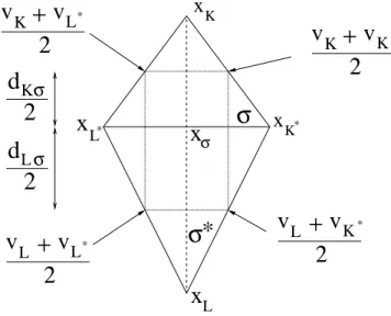
Definition 3.3. Let v = ((vK)K∈T, (vσ)σ∈Eext, (vK∗)K∗∈T∗) be in V0(T ) defined above. With these values, we
define a function vh constructed in the following way. Let us first consider an inner primal edge σ ∈ Eint with
σ = K|L and σ∗ = K∗|L∗ its associated inner dual edge. The restriction of v
h on Vσ,σ∗ is defined as the only
P1 function over V
σ,σ∗ which is such that (see Fig. 5)
vh µ xK+ xK∗ 2 ¶ = vK+ vK∗ 2 , vh µ xK+ xL∗ 2 ¶ = vK+ vL∗ 2 , vh µ xL+ xL∗ 2 ¶ = vL+ vL∗ 2 , vh µ xL+ xK∗ 2 ¶ = vL+ vK∗ 2 . (14)
A similar formula defines vhon Vσ,σ∗ if σ ∈ Eextwith σ ⊂ ∂K ∩ Γ associated to the inner dual edge σ∗= K∗|L∗:
vh µ xK+ xK∗ 2 ¶ = vK+ vK∗ 2 , vh µ xK+ xL∗ 2 ¶ = vK+ vL∗ 2 , vh µ xσ+ xL∗ 2 ¶ = vσ+ vL∗ 2 , vh µ xσ+ xK∗ 2 ¶ = vσ+ vK∗ 2 . (15)
Of course, the definition of a P1 function by four of its values is in general impossible. However, it may be
checked that (see [19, Prop. 4.1] for details), in the present case, such a function exists and is unique thanks to the fact that the quadrangle xK+xK∗
2 xK+x2 L∗ xL+x2 L∗ xL+x2K∗ is a rectangle (actually, a parallelogram would
be enough) and since the four prescribed values in the right-hand sides of (14) are not independent but verify vK+ vK∗ 2 + vL+ vL∗ 2 = vK+ vL∗ 2 + vL+ vK∗ 2 .
Note that the function vh is non-conforming since it is only continuous at the midpoints of the boundaries of
the cells Vσ,σ∗. Note that thanks to the second line in (15), and since vσ= 0 for all σ ∈ Eext and vK∗ = 0 for
all K∗∈ T∗
ext, the function vh vanishes on Γ.
Definition 3.4. We call L the linear operator which associates to the element v ∈ V0(T ) the function vhdefined
above. Next, we define
Vh0:= L(V0(T ))
the set of all possible functions vh defined by (14) and (15).
x
Kv
Κ+
v
Κ*2
v
L+
v
L2
*σ
d
K2
σ
d
L2
σ
σ
*
L*x
x
K*x
Lx
σv
Κ+
v
2
v
+
v
Κ* L2
L*Figure 5. Values of the P1 function v
h on the diamond-cell Vσ,σ∗.
Proposition 3.5. Let vh be in Vh0. Then its broken (diamond-cell per diamond-cell) gradient ∇hvh has the
following expression (∇hvh)Vσ,σ∗ = (vL− vK) dσ nKL+ (vL∗ − vK∗) m(σ) nK∗L∗ if σ ∈ Eint (vσ− vK) dσ nKσ+ (vL∗− vK∗) m(σ) nK∗L∗ if σ ∈ Eext , ∀Vσ,σ∗. (16)
We may now state the main result of this section
Proposition 3.6. The finite volume formulations (4)–(11) may be combined into a single finite element-like
formulation which reads: Find uh in Vh0 such that for all vh in Vh0,
ah(uh, vh) = ℓ(v△,∗h ) , (17) where ah(uh, vh) = X Vσ,σ∗ Z Vσ,σ∗ ∇huh · ∇hvhdx and ℓ(vh△,∗) = Z Ω f v△,∗h (x) dx . (18)
Moreover, there exists a constant C not depending on the mesh such that, if ˆu is in H2(Ω), there holds
|ˆu − uh|1,h:= ah(ˆu − uh, ˆu − uh)1/2≤ Ch kˆukH2(Ω). (19)
Note that the definitions of the bilinear form ah and of the linear form ℓ may be extended to functions
belonging to H1(Ω). For such functions, the broken gradient in the definition of a
h should be replaced by the
classical continuous gradient ∇.
Proof. The equivalence between the finite element like formulation and the finite volume schemes is a particular
Consider any vector v = ((vK)K∈T, (vσ)σ∈Eext, (vK∗)K∗∈T∗) in V0(T ). Thanks to (4) and (7), there holds −vK X σ∈EK FK,σ= m(K)vKfK = Z Ω f (x)vKθK(x)dx , ∀K ∈ T .
Then, thanks to (8) and (11), there holds for all K∗∈ T∗ int −vK∗ X σ∗∈EK∗ FK∗,σ∗ = m(K∗)vK∗fK∗ = Z Ω f (x)vK∗θK∗(x)dx . (20)
But since vK∗ vanishes for all K∗∈ Text∗ , we may also write, for K∗∈ Text∗
−vK∗ X σ∗∈EK∗∩E∗ int FK∗,σ∗ = Z Ω f (x)vK∗θK∗(x)dx .
Thus, for any vector v in V0(T ), there holds
−12 X K∈T vK X σ∈EK FK,σ+ X K∗∈T∗ vK∗ X
σ∗∈EK∗∩Eint∗
FK∗,σ∗ = Z Ω f v△,∗h (x)dx . (21)
Now the sums in the left-hand side of Eq. (21) can be reorganized in the following way. Let us first consider a given σ ∈ Eint and its associated σ∗ ∈ Eint∗ . They both appear twice in the sums in the left-hand side of
Eq. (21). Since FK,σ= −FL,σ and FK∗,σ∗ = −FL∗,σ∗ if σ = K|L and σ∗= K∗|L∗, we may write, thanks to the
expressions of FK,σand FK∗,σ∗, respectively given by (5) and (9)
−12(vKFK,σ+ vLFL,σ+ vK∗FK∗,σ∗+ vL∗FL∗,σ∗) = 1 2m(σ) (uL− uK) dσ (vL− vK) + 1 2dσ (uL∗− uK∗) m(σ) (vL∗− vK∗) = m(Vσ,σ∗) · (uL− uK) dσ (vL− vK) dσ +(uL∗ − uK∗) m(σ) (vL∗ − vK∗) m(σ) ¸ ,
thanks to (1). Let us now consider a given σ ∈ Eext and its associated σ∗∈ Eint∗ . In Eq. (21), σ appears only
once since it is a boundary edge. On the other hand, σ∗ still appears twice and we may write
−12(vKFK,σ+ vK∗FK∗,σ∗+ vL∗FL∗,σ∗) = −12m(σ)(uσ− uK) dσ vK+ 1 2dσ (uL∗− uK∗) m(σ) (vL∗ − vK∗) = m(Vσ,σ∗) · (uσ− uK) dσ (vσ− vK) dσ +(uL∗ − uK∗) m(σ) (vL∗− vK∗) m(σ) ¸ , since vσ vanishes. Finally, since nKL· nK∗L∗ = 0, Eq. (21) may be rewritten as
X Vσ,σ∗ m(Vσ,σ∗) (∇huh)V σ,σ∗ · (∇hv)Vσ,σ∗ = X Vσ,σ∗ Z Vσ,σ∗ ∇huh· ∇hvh= Z Ω f v△,∗h (x)dx ,
Moreover, the error estimation (19) is inferred from [19, Th. 5.20], in which the angle τ∗ is always equal to
π/2 in the special case of Delaunay-Voronoi meshes. Related convergence results in a discrete norm for each
component (primal or dual) of the gradient may be found in [22, 33, 37]. ¤
4.
Error estimation in the L
2norm
Using the equivalent (non-conforming) finite element formulation, we shall derive an estimation in the L2
norm using the traditional Aubin-Nitsche lemma. An additional difficulty will arise due to the fact that the right-hand side in (17) is given by (18) instead of the more traditional term R
Ωf vh(x) dx which would arise
in a genuine finite element method. In order to evaluate errors coming from the difference between these two terms, we shall state a regularity hypothesis on f , which is the same as that involved in the studies concerning vertex-centered finite volume element schemes, see, e.g., [21] and one-dimensional cell-centered finite volume schemes, see [35].
Hypothesis 4.1. We suppose that the function f belongs to H1(Ω).
Remark 4.2. The first consequence of this hypothesis (actually, f in L2(Ω) would be enough for this) is that,
since Ω has been supposed to be a convex polygonal domain, the exact solution ˆu of the Laplace equation belongs to H2(Ω) and there exists a constant C, not depending in f such that kˆuk
H2(Ω) ≤ C kfkL2(Ω). As a
corollary, the error estimation (19) provides
|ˆu − uh|1,h ≤ Ch kfkL2(Ω) , (22)
with a constant C that does not depend on the mesh.
4.1. A representation formula for the error in the L
2(Ω) norm
We start by writing kˆu − uhkL2(Ω)= sup g∈L2(Ω) R Ω(uh− ˆu)g(x)dx kgkL2(Ω) . (23)Now, for a given g ∈ L2(Ω), let us define ˆφ ∈ H1
0(Ω) which is the unique solution of the following problem
½
−∆ ˆφ = g in Ω ˆ
φ = 0 on Γ . (24)
Since g is in L2(Ω), and since we have supposed that Ω is a convex polygonal domain, ˆφ belongs to H2(Ω) and
there exists a constant C depending only on Ω such that ° ° ° ˆ φ°° °H2(Ω)≤ C kgkL2(Ω) . (25)
We may write the following representation formula
Proposition 4.3. Let φ = ((φK)K∈T, (φσ)σ∈Eext, (φK∗)K∗∈T∗) be given in V0(T ) and let
be the function associated to φ through Def. 3.4. There holds Z Ω (uh− ˆu)g(x)dx = ah(uh− ˆu, ˆφ − φh) − Z Ω f³φh− φ△,∗h ´ (x) dx − X Vσ,σ∗ Z ∂Vσ,σ∗ ∇ˆu · n φhdσ (27) − X Vσ,σ∗ Z ∂Vσ,σ∗ (uh− ˆu) ∇ ˆφ · n dσ .
Proof. Through Eq. (24), there holds
Z Ω (uh− ˆu)g(x)dx = − X Vσ,σ∗ Z Vσ,σ∗ (uh− ˆu) ∆ ˆφ (x) dx = ah(uh− ˆu, ˆφ) − X Vσ,σ∗ Z ∂Vσ,σ∗ (uh− ˆu) ∇ ˆφ · n dσ, (28)
thanks to a Green formula on each Vσ,σ∗, and where n is the unit exterior normal vector on ∂Vσ,σ∗. Now let us
consider an arbitrary φ given in V0(T ) and let φh= L(φ) be its associated function. There holds, by definition
of the bilinear form ah
ah(uh− ˆu, ˆφ) = ah(uh− ˆu, ˆφ − φh) + ah(uh, φh) − X Vσ,σ∗ Z Vσ,σ∗ ∇ˆu · ∇hφh(x)dx . (29) Thanks to (17), we have ah(uh, φh) = Z Ω f φ△,∗h (x)dx . (30)
On the other hand, since −∆ˆu = f, a Green formula on each Vσ,σ∗ provides
− X Vσ,σ∗ Z Vσ,σ∗ ∇ˆu · ∇hφh(x)dx = − X Vσ,σ∗ Z Vσ,σ∗ f φh(x)dx − X Vσ,σ∗ Z ∂Vσ,σ∗ ∇ˆu · n φhdσ . (31)
Gathering (28)–(31), the result (27) is obtained. ¤
Up to now, the values of φ are arbitrary, but since they will play a key role in the evaluation of the various terms in (27), we shall precise them now.
4.2. Choosing φ
Of course, we shall choose φ so that the associated function φh = L(φ) (see Def. 3.4) will be a good
approximation of ˆφ. We propose to choose the values ((φK)K∈T, (φσ)σ∈Eext, (φK∗)K∗∈T∗) as the solutions of
the primal and dual finite volume schemes of section 2, associated to the Laplace equation (24) satisfied by ˆφ. More precisely, we write
− X σ∈EK FK,σ= Z Kg(x)dx, , ∀K ∈ T , (32) with the fluxes
FK,σ= m(σ)
(φL− φK)
dσ , if σ ∈ Eint, σ = K|L ,
FK,σ= m(σ)(φσ− φK)
dσ , if σ ∈ E
ext, σ ⊂ ∂K ∩ Γ . (34)
In (34), we set
φσ = 0 (35)
according to the homogeneous Dirichlet boundary condition. The second scheme reads
− X σ∗∈E K∗ FK∗,σ∗ = Z K∗g(x)dx , ∀K ∗ ∈ Tint∗ , (36)
with the fluxes
FK∗,σ∗ = dσ
(φL∗ − φK∗)
m(σ) , if σ
∗
∈ Eint∗ , σ∗= K∗|L∗ (37)
and boundary conditions
φK∗ = 0 , ∀K∗∈ Text∗ . (38)
Note that Eqs (35) and (38) ensure that φ is indeed in V0(T ) as required in Prop. 4.3.
In particular, two points will be important in what follows. First, since ˆφ is in H2(Ω), we may apply the
error estimate given by (19), in which we replace ˆu and uhby ˆφ and φh, so that there holds, taking into account
(25) ¯ ¯ ¯φ − φˆ h ¯ ¯ ¯ 1,h ≤ Ch kgkL2(Ω) . (39)
with a constant C not depending on the mesh. Moreover, it is clear from the definitions (16) and from (32) and (33), that φh verifies − X σ∈EK m(σ)∇hφh· nKσ= Z Kg(x)dx, , ∀K ∈ T . (40) For this, we recall that we have set nKL= nKσ if σ = K|L.
4.3. Estimations of the various terms in (27)
The technique used to evaluate the last two terms in Eq. (27) is classical and dates back to [17]. It is based on [17, lemma 3], in which we choose m = 0:
Lemma 4.4. Let T be a triangle and let T′ be any of its edges; there exists a constant C independent of T such
that for all v in H1(T ), and for all ϕ in H1(T ), there holds
¯ ¯ ¯ ¯ Z T′ ϕ(v − MT′v) dσ ¯ ¯ ¯ ¯≤ Cσ(T ) diam(T ) |ϕ|1,T|v|1,T , (41) where MT′v := m(T1′) R
T′v dσ is the mean value of v over T
′ and where σ(T ) := diam(T )
ρ(T ) is classically the ratio
of the diameter of T to the diameter of the largest circle inscribed in T .
Let us start by the last term in (27).
Lemma 4.5. There exists a constant C depending only on θ∗ such that
¯ ¯ ¯ ¯ ¯ ¯ X Vσ,σ∗ Z ∂Vσ,σ∗ (uh− ˆu) ∇ ˆφ · n dσ ¯ ¯ ¯ ¯ ¯ ¯ ≤ Ch2 kfkL2(Ω) kgkL2(Ω) . (42)
* K
x
x
σ Kx
T
T’
Figure 6. Definition of the triangle T and its edge T′.
Proof. The function uhis piecewise P1and continuous at the midpoint of each edge of the diamond mesh and
vanishes on the boundary Γ. Moreover, ˆφ is in H2(Ω). Thus, there holds
X Vσ,σ∗ X T′⊂∂Vσ,σ∗ Z T′ uhMT′∇ ˆφ · n = 0 .
Moreover, since ˆu is in H2(Ω) and vanishes on Γ
X Vσ,σ∗ X T′⊂∂Vσ,σ∗ Z T′ ˆ u MT′∇ ˆφ · n = 0 . Therefore, X Vσ,σ∗ Z ∂Vσ,σ∗ (uh− ˆu) ∇ ˆφ · n dσ = X Vσ,σ∗ X T′⊂∂Vσ,σ∗ Z T′ (uh− ˆu) (∇ ˆφ · n − MT′∇ ˆφ · n) dσ .
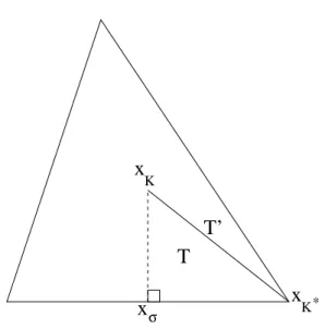
Next, for each Vσ,σ∗ and each edge T′ ⊂ ∂Vσ,σ∗, we shall apply lemma 4.4 on a triangle T defined to be the
convex hull of T′∪ {xσ} (see Fig. 6) with v = ∇ ˆφ · n ∈ H1(T ) (since ˆφ ∈ H2(Ω)) and ϕ = (uh− ˆu) ∈ H1(T )
(since uhis in P1(T ) and ˆu ∈ H2(Ω)). Since diam(T ) ≤ h and since it is well-known that σ(T ) ≤ sin θ(T )2 where
θ(T ) is the smallest angle in T , the second point of lemma 1.2 and (41) lead to the existence of a constant C depending only on θ∗ such that
¯ ¯ ¯ ¯ Z T′ (uh− ˆu) (∇ ˆφ · n − MT′∇ ˆφ · n) dσ ¯ ¯ ¯ ¯≤ Ch k∇(ˆu − uh)kL2(T ) ° ° °φˆ ° ° °H2(T ) .
Since the set of such triangles T constitutes a partition of Ω, a discrete Cauchy-Schwarz inequality, together
with (25) and (22) leads to (42). ¤
Lemma 4.6. There exists a constant C depending only on θ∗ such that ¯ ¯ ¯ ¯ ¯ ¯ X Vσ,σ∗ Z ∂Vσ,σ∗ ∇ˆu · n φhdσ ¯ ¯ ¯ ¯ ¯ ¯ ≤ Ch2kfkL2(Ω) kgkL2(Ω) . (43)
Proof. The third term in the right-hand side of (27) may be transformed into
− X
Vσ,σ∗
Z
∂Vσ,σ∗
∇ˆu · n (φh− ˆφ) dσ (44)
since ˆφ is continuous and vanishes along Γ and since there is no jump of ∇ˆu ∈ H1(Ω) across ∂V
σ,σ∗. Now, the
technique we have used above to obtain (42) may be applied to evaluate (44) and we end up with ¯ ¯ ¯ ¯ ¯ ¯ X Vσ,σ∗ Z ∂Vσ,σ∗ (φh− ˆφ) ∇ˆu · n dσ ¯ ¯ ¯ ¯ ¯ ¯ ≤ Ch¯¯ ¯φ − φˆ h ¯ ¯ ¯1,hkfkL2(Ω)
with a constant depending only on θ∗, and we conclude with (39). ¤
Next, bounding the first term in the right-hand side of (27) is performed by the Cauchy-Schwarz inequality and by (22) and (39). We obtain
Lemma 4.7. There exists a constant C not depending on the mesh such that ¯ ¯ ¯ah(uh− ˆu, ˆφ − φh) ¯ ¯ ¯ ≤ C h 2 kfk L2(Ω) kgkL2(Ω) . (45)
Now, the term which remains to be evaluated in (27) is that coming from the fact that (17)-(18) is not a genuine finite element formulation, like explained in the introduction of section 4.
We shall first define the following functions
Definition 4.8. Let ((φK)K∈T, (φσ)σ∈Eext, (φK∗)K∗∈T∗) be given, we define φ △ h and φ∗h by φ△h |K(x) :=φK 2 , ∀x ∈ K , ∀K ∈ T , (46) φ∗ h|K∗(x) := φK∗ 2 , ∀x ∈ K ∗, ∀K∗∈ T∗, (47)
Definition 4.9. Let ((φK)K∈T, (φσ)σ∈Eext, (φK∗)K∗∈T∗) be given, we define φ 1 h and φ2hby φ1h(x)|Vσ,σ∗ := dKσφL+ dLσφK 2dσ + (x − xσ) · µ φL− φK dσ ¶ nKL, ∀x ∈ Vσ,σ∗ if σ = K|L ∈ Eint φσ 2 + (x − xσ) · µ φσ− φK dσ ¶ nKσ, ∀x ∈ Vσ,σ∗ if σ ∈ Eext , (48) and φ2 h(x)|Vσ,σ∗ := φL∗+ φK∗ 4 + (x − xσ) · µ φL∗− φK∗ m(σ) ¶ nK∗L∗, ∀x ∈ Vσ,σ∗ , with σ∗= K∗|L∗, (49)
With these definitions, there holds Lemma 4.10. φh− φ△,∗h = ³ φ1h− φ △ h ´ +¡φ2 h− φ∗h¢ . (50)
Proof. From (13), (46) and (47), there holds
φ△,∗h (x) = φ△h(x) + φ∗h(x) , ∀x ∈ Ω . (51)
Moreover, the following equality may also be easily checked by simple interpolation (see Fig. 5)
φh(xσ) = dKσφL+ dLσφK 2dσ + φL∗+ φK∗ 4 if σ = K|L ∈ Eint, σ ∗= K∗ |L∗ φσ 2 + φL∗+ φK∗ 4 if σ ∈ Eext, σ ∗= K∗ |L∗
so that, since φhis a P1 function in Vσ,σ∗,
φh(x)|Vσ,σ∗ = dKσφL+ dLσφK 2dσ + φL∗ + φK∗ 4 + (x − xσ) · ∇hφh, ∀x ∈ Vσ,σ∗ if σ = K|L ∈ Eint φσ 2 + φL∗ + φK∗ 4 + (x − xσ) · ∇hφh, ∀x ∈ Vσ,σ∗ if σ ∈ Eext ,
with, in both cases, σ∗= K∗|L∗. Recalling that ∇
hφhis given by (16), and with the definitions (48) and (49),
there holds φh(x)|Vσ,σ∗ = φ 1 h(x)|Vσ,σ∗ + φ 2 h(x)|Vσ,σ∗,
which, together with (51), leads to (50). ¤
Moreover, from (48), (49) and (16), recalling that we have set nKL= nKσ if σ = K|L, there holds
Lemma 4.11. (∇hφ1h)|Vσ,σ∗ · nKσ= µ φL− φK dσ ¶ = (∇hφh)|Vσ,σ∗ · nKσ if σ = K|L ∈ Eint µ φσ− φK dσ ¶ = (∇hφh)|Vσ,σ∗ · nKσ if σ ∈ Eext (52) and (∇hφ2h)|Vσ,σ∗ · nK∗L∗ = µ φL∗− φK∗ m(σ) ¶ = (∇hφh)|Vσ,σ∗ · nK∗L∗. (53)
With these definitions, the remaining term which has to be evaluated in (27) reads Z Ω f³φh− φ△,∗h ´ (x) dx = Z Ω¡f − f △¢³ φ1h− φ △ h ´ (x) dx + Z Ω f△³φ1h− φ △ h ´ (x) dx + Z Ω ³ f − fσσ∗´¡φ2 h− φ∗h¢ (x) dx (54) + Z Ω fσσ∗¡φ2 h− φ∗h¢ (x) dx ,
where the following L2 projections have been used:
f△(x) = f K = 1 m(K) Z Kf (x)dx , ∀x ∈ K , ∀K ∈ T , (55)
fσσ∗(x) = fVσ,σ∗ = 1 m(Vσ,σ∗) Z Vσ,σ∗ f (x)dx , ∀x ∈ Vσ,σ∗, ∀Vσ,σ∗.
We shall first evaluate the first and third terms in the right-hand side of Eq. (54). Lemma 4.12. There exists a constant C, not depending on the mesh, such that
¯ ¯ ¯ ¯ Z Ω¡f − f △¢³ φ1h− φ △ h ´ (x) dx + Z Ω ³ f − fσσ∗´¡φ2 h− φ∗h¢ (x) dx ¯ ¯ ¯ ¯≤ Ch 2 kfkH1(Ω)kgkL2(Ω). (56)
Proof. From (48), if σ ∈ Eint, with σ = K|L, there holds
φ1h µ xK+ xσ 2 ¶ = dKσφL+ dLσφK 2dσ +µ xK− xσ 2 ¶ ·µ φL− φd K σ ¶ nKL = dKσφL+ dLσφK 2dσ − dKσ(φL− φK) 2dσ = dKσ+ dLσ 2dσ φK = φK 2 = φ △ h |K, (57)
and the same equality holds if σ ∈ Eext, with σ ⊂ ∂K ∩ ∂Ω. This shows that the function φ△h interpolates the
function φ1
hat xK+x2 σ ∈ VK,σ. Thus, since φ1h− φ △
h is a P1 function in VK,σ, there holds, with (52)
° ° °φ 1 h− φ △ h ° ° ° 2 L2(VK,σ) ≤ diam2(VK,σ) ° °∇hφ1h ° ° 2 L2(VK,σ)≤ diam 2 (VK,σ) k∇hφhk2L2(VK,σ).
Summing over all VK,σ for σ ∈ EK and K ∈ T , and since diam(VK,σ) ≤ h, we obtain
° ° °φ 1 h− φ △ h ° ° ° L2(Ω)≤ h |φh|1,h .
In the same way, it may be shown from (49) that φ∗
h interpolates φ2hat xK⋆2+xσ ∈ VK∗,σ∗, so that ° °φ2 h− φ∗h ° ° L2(Ω)≤ h |φh|1,h .
On the other hand, since, through Hyp. 4.1, f ∈ H1(Ω), and since every K and every V
σ,σ∗ are convex, there
exists a constant C that does not depend on f , K or Vσ,σ∗ such that
° °f − f△ ° °L2(K)≤ Cdiam(K) k∇fkL2(K) and ° ° °f − f σσ∗° ° °L2(V σ,σ∗) ≤ Cdiam(Vσ,σ∗) k∇fkL2(Vσ,σ∗). This leads to ° °f − f△ ° ° L2(Ω)≤ Ch k∇fkL2(Ω) and ° ° °f − f σσ∗° ° °L2(Ω)≤ Ch k∇fkL2(Ω). We conclude that ¯ ¯ ¯ ¯ Z Ω¡f − f △¢³ φ1h− φ △ h ´ (x) dx + Z Ω ³ f − fσσ∗´¡φ2 h− φ∗h¢ (x) dx ¯ ¯ ¯ ¯≤ Ch 2 k∇fkL2(Ω)|φh|1,h , (58)
Moreover, the triangle inequality and (39) lead to |φh|1,h ≤ ° ° °φˆ ° ° °H1(Ω)+ ¯ ¯ ¯φ − φˆ h ¯ ¯ ¯1,h ≤ ° ° °φˆ ° ° °H2(Ω)+ Ch||g||L2(Ω), (59)
which, injected in (58), and taking (25) into account, lead to (56). ¤
We now evaluate the last term in Eq. (54).
Lemma 4.13. There holds Z
Ω
fσσ∗¡φ2
h− φ∗h¢ (x) dx = 0 . (60)
Proof. Since fσσ∗ is a constant over each Vσ,σ∗, there holds
Z Ω fσσ∗ ¡φ2 h− φ∗h¢ (x) dx = X Vσ,σ∗ fVσ,σ∗ Z Vσ,σ∗ ¡φ2 h− φ∗h¢ (x) dx. (61)
Since xσ is the midpoint of σ, and by symmetry of Vσ,σ∗ with respect to [xKxL], there holds
Z
Vσ,σ∗
(x − xσ) · nK∗L∗dx = 0 .
Thus, from Eq. (49), we infer that Z
Vσ,σ∗
φ2h(x)dx = m(Vσ,σ∗)
φL∗ + φK∗
4 . (62)
Moreover, from Eq. (47) Z Vσ,σ∗ φ∗h(x)dx = Z VK∗ ,σ∗ φK∗ 2 dx + Z VL∗ ,σ∗ φL∗ 2 dx .
By symmetry of Vσ,σ∗ with respect to [xKxL], there holds m(VK∗,σ∗) = m(VL∗,σ∗) = 12m(Vσ,σ∗). Thus,
Z
Vσ,σ∗
φ∗h(x)dx = m(Vσ,σ∗)
φL∗+ φK∗
4 . (63)
Thus, (60) follows from (61), (62) and (63). ¤
Finally, there remains to evaluate the second term in the right-hand side of (54). The following lemma will be helpful for this.
Lemma 4.14. Recall that RK is the radius of the circle in which the triangle K is inscribed. There holds
Z Ω f△³φ1h− φ △ h ´ (x) dx = X K∈T fK R2 K 12 X σ∈EK m(σ)∇hφh· nKσ − 481 X K∈T fK X σ∈EK (m(σ))3∇hφh· nKσ. (64)
Proof. By definition of φ△h, see (46), and of f△, see (55), there holds
Z Ω f△³φ1h− φ △ h ´ (x) dx = X K∈T fK X σ∈EK Z VK,σ µ φ1h− φK 2 ¶ (x) dx . (65)
Since φ1
h is a P1 function over the triangle VK,σ, the following quadrature formula is exact
Z VK,σ φ1h(x)dx = m(V K,σ) 3 £φ 1 h(xK) + 2φ1h(xσ)¤ . (66)
But we also have
φ1h(xK) + φ1h(xσ) = 2φ1h µ xK+ xσ 2 ¶ (67) and φ1 h(xσ) = φ1h µ xK+ xσ 2 ¶ +xσ− xK 2 · ∇hφ 1 h. (68)
Summing (67) and (68), and using (57), the fact that xσ− xK= dKσnKσ and (52), Eq. (66) writes
Z VK,σ φ1h(x)dx = m(VK,σ) 3 · 3φK 2 + dKσ 2 ∇hφh· nKσ ¸ .
Since m(VK,σ) = dKσ2m(σ), we finally have
Z VK,σ µ φ1h− φK 2 ¶ (x) dx = d 2 Kσm(σ) 12 ∇hφh· nKσ. The next step is the calculation of
X σ∈EK Z VK,σ µ φ1h− φK 2 ¶ (x) dx = X σ∈EK d2 Kσm(σ) 12 ∇hφh· nKσ.
This is performed using the fact that d2
Kσ= R2K− (m(σ))2
4 (see Fig. 1). Thus,
X σ∈EK Z VK,σ µ φ1h− φK 2 ¶ (x) dx = R 2 K 12 X σ∈EK m(σ)∇hφh· nKσ − 481 X σ∈EK (m(σ))3∇hφh· nKσ. (69)
Inserting (69) into (65) yields (64). ¤
Now, we bound the first term in the right-hand side of (64). Lemma 4.15. There exists a constant C such that
¯ ¯ ¯ ¯ ¯ X K∈T fK R2 K 12 X σ∈EK m(σ)∇hφh· nKσ ¯ ¯ ¯ ¯ ¯ ≤ Ch2kfkL2(Ω)kgkL2(Ω). (70)
Proof. Recall that φ has been chosen so that (40) holds. This implies
R2K X σ∈EK m(σ)∇hφh· nKσ= −R2K Z K g(x)dx
so that, using a continuous and then a discrete Cauchy-Schwarz inequality, ¯ ¯ ¯ ¯ ¯ X K∈T fK R2 K 12 X σ∈EK m(σ)∇hφh· nKσ ¯ ¯ ¯ ¯ ¯ ≤ 121 X K∈T fKR2Kpm(K) kgkL2(K) ≤ 121 h2 Ã X K∈T m(K) |fK|2 !1/2 kgkL2(Ω),
since RK ≤ h by definition. Eq. (70) is then obtained since
³ P
K∈T m(K) |fK|2
´1/2
≤ kfkL2(Ω). ¤
Lemma 4.16. Under Hyp. 1.1 and 4.1, there exists a constant C, depending only on θ∗, such that
¯ ¯ ¯ ¯ ¯ 1 48 X K∈T fK X σ∈EK (m(σ))3∇hφh· nKσ ¯ ¯ ¯ ¯ ¯ ≤ Ch2kfkH1(Ω)kgkL2(Ω) . (71)
Proof. Recall that for any σ = K|L, there holds ∇hφh· nKL= −∇hφh· nLK. Thus,
X K∈T fK X σ∈EK (m(σ))3∇hφh· nKL = X σ∈Eint,σ=K|L (m(σ))3(fK− fL) ∇hφh· nKL + X σ∈Eext (m(σ))3fK∇hφh· nKL. (72)
Since m(Vσ,σ∗) =m(σ) d2 σ, and m(σ) ≤ h there holds
(m(σ))3=√2qm(Vσ,σ∗)(m(σ))2 s m(σ) dσ ≤ Ch 2q m(Vσ,σ∗) s m(σ) dσ , so that, using a discrete Cauchy-Schwarz inequality yields
¯ ¯ ¯ ¯ ¯ ¯ X σ∈Eint,σ=K|L (m(σ))3(fK− fL) ∇hφh· nKL ¯ ¯ ¯ ¯ ¯ ¯ ≤ Ch2 X σ∈Eint,σ=K|L m(σ) dσ (fK− fL)2 1/2 |φh|1,h .
Thanks to the last point of Lemma 1.2, we may now directly apply [22, Lemma 9.4] to conclude that ¯ ¯ ¯ ¯ ¯ ¯ X σ∈Eint,σ=K|L (m(σ))3(f K− fL) ∇hφh· nKL ¯ ¯ ¯ ¯ ¯ ¯ ≤ Ch2kfk H1(Ω)|φh|1,h .
Using (59) and taking (25) into account, this yields ¯ ¯ ¯ ¯ ¯ ¯ X σ∈Eint,σ=K|L (m(σ))3(fK− fL) ∇hφh· nKL ¯ ¯ ¯ ¯ ¯ ¯ ≤ Ch2kfkH1(Ω)kgkL2(Ω). (73)
Now the last term in (72) may be estimated in the following way X σ∈Eext (m(σ))3fK∇hφh· nKL= X σ∈Eext (m(σ))3 m1/2(K)m1/2(V σ,σ∗) m1/2(K)fKm1/2(Vσ,σ∗)∇hφh· nKL. (74)
Since for boundary triangles Vσ,σ∗ = VK,σ⊂ K, there holds m1/2(K)m1/2(Vσ,σ∗) ≥ m(VK,σ) =m(σ)dKσ 2 , so that (m(σ))3 m1/2(K)m1/2(V σ,σ∗) ≤ 2 (m(σ))2 dKσ ≤ Ch ,
with a constant depending only on θ∗, thanks to the last point in lemma 1.2. Taking this into account in (74)
and applying a discrete Cauchy-Schwarz inequality, there holds ¯ ¯ ¯ ¯ ¯ X σ∈Eext (m(σ))3fK∇hφh· nKL ¯ ¯ ¯ ¯ ¯ ≤ Ch k∇hφhkL2(Bh)kfkL2(Bh), (75)
since fK is the L2orthogonal projection of f over K. We have denoted by Bhthe strip around Γ which contains
all K such that m(∂K ∩ Γ) 6= 0. Note that this strip has a width of at most h, so that, according to Ilin’s inequality (see, e.g. [12, Formula (2.1)]), and since ˆφ ∈ H2(Ω), there holds
° ° °∇φˆ ° ° °L2(B h) ≤ Ch1/2°° °φˆ ° ° °H2(Ω) , which implies k∇hφhkL2(Bh) ≤ ¯ ¯ ¯φh− ˆφ ¯ ¯ ¯ 1,h+ ° ° °∇φˆ ° ° ° L2(Bh) ≤ Ch kgkL2(Ω)+ Ch1/2 ° ° ° ˆ φ°° °H2(Ω)≤ Ch 1/2kgk L2(Ω), (76)
according to (39). Moreover, since by Hyp. 4.1, f belongs to H1(Ω), we may apply Ilin’s inequality again to
obtain
kfkL2(Bh)≤ Ch1/2kfkH1(Ω). (77)
Inserting (76) and (77) into (75), we conclude that there exists a constant C such that ¯ ¯ ¯ ¯ ¯ X σ∈Eext (m(σ))3fK∇hφh· nKL ¯ ¯ ¯ ¯ ¯ ≤ Ch2kgkL2(Ω)kfkH1(Ω) . (78)
Gathering (78) and (73) into (72) yields (71). ¤
Starting from (23), we may now gather all the intermediary results (27), (42), (43), (45), (54), (56), (60), (64), (70) and (71) to get the main result of this article
Theorem 4.17. Let Ω be a two-dimensional convex polygonal domain. Let ˆu be the exact solution of the equation −∆ˆu = f in Ω, with homogeneous Dirichlet boundary conditions. Let u = ((uK)K∈T, (uσ)σ∈Eext, (uK∗)K∗∈T∗)
be the solution of the finite volumes schemes (4)–(11), and let uh be the function in Vh0 associated to u through
definitions 3.3 and 3.4. Then, under Hyp. 1.1 and 4.1, there exists a constant C depending only on θ∗, such
that
5.
Extension to a more general diffusion equation
The question of extending the result presented in this article to more general situations actually contains three sub-questions: a) What would the finite volume schemes in these more general situations be? b) Given these FV schemes, can they be recast into an equivalent finite element - like scheme? c) From this equivalent scheme, is it possible to infer second order convergence?
In case of a diffusion equation −∇ · (η∇ˆu) = f with a regular scalar coefficient η, the usual answer to sub-question a) is that in equations (4) and (8) the fluxes are now defined in the following way (we restrict the discussion to inner edges for the sake of simplicity):
FK,σ = m(σ)ησ (uL− uK) dσ , if σ = K|L FK∗,σ∗ = dσησ∗ (uL∗− uK∗) m(σ) , if σ ∗= K∗ |L∗
Several choices may be proposed for ησ and ησ∗; for example the choice
ησ = 1 m(σ) Z σ η dℓ ησ∗ = 1 dσ Z σ∗ η dℓ
corresponds to mean-values of η along the edges (see, e.g., Ref. [6]). Another possibility is suggested by Ref. [22, pp. 816–818]: ησ = ηKηLdσ ηKdLσ+ ηLdKσ ησ∗ = 2ηK∗ηL∗ ηK∗ + ηL∗ ,
which corresponds to harmonic averaging of cell-defined values ηK, ηL, ηK∗ and ηL∗ which may themselves be
defined as mean-values of η over the respective associated cells.
Regarding sub-question b), it may be checked that the resulting FV schemes may be rewritten into a finite element - like scheme which reads
ah(uh, vh) = ℓ(vh∆,∗),
where the definition of the bilinear form ahis now given by
ah(uh, vh) := X Vσ,σ∗ Z Vσ,σ∗ (Aσ,σ∗∇huh) · ∇hvh
where, if we denote by (nxKL, nyKL) the coordinates of the normal vector nKL, the diamond-cell dependent
matrix Aσ,σ∗ is defined by Aσ,σ∗ = µ ησn2xKL+ ησ∗nyKL2 (ησ− ησ∗)nxKLnyKL (ησ− ησ∗)nxKLnyKL ησ∗n2xKL+ ησn2yKL ¶ .
Although this is not a very natural finite element - like technique, this is still acceptable because if η is regular, then Aσ,σ∗ = η(x)Id + O(h). We may admit that if η is regular, uniformly strictly positive and bounded then
However, we may now face a difficulty coming from point c). Indeed, the first line of Eq. (24) is now replaced by −∇ · (η∇ ˆφ) = g, and for a sufficiently regular η and a polygonal convex domain, there holds ˆφ ∈ H1
0(Ω) ∩ H2(Ω)
with
|| ˆφ||H2(Ω)≤ C||g||L2(Ω) (80)
and we may prove that (27) is replaced by Z Ω (uh− ˆu)g(x)dx = X Vσ,σ∗ Z Vσ,σ∗ η (∇huh− ∇ˆu) · (∇ ˆφ − ∇hφh)(x)dx − Z Ω f (φh− φ∆,∗h ) + X Vσ,σ∗ Z Vσ,σ∗ (η(x) Id − Aσ,σ∗)∇huh· ∇hφhdx (81) − X Vσ,σ∗ Z ∂Vσ,σ∗ η ∇ˆu · n φh(x) dℓ − X Vσ,σ∗ Z ∂Vσ,σ∗ (uh− ˆu) η ∇ ˆφ · n(x) dℓ.
All but the third term of the above formula are similar to Eq. (27) and may be treated with small modifications that we detail now.
First, we choose the discrete φ (and its associated reconstruction φh) as the solution of both finite volume
schemes associated to the solution of the Laplace equation with right-hand side ˜g := −∆ ˆφ. It holds that ˜g belongs to L2(Ω) since ˆφ is in H2(Ω) and
||˜g||L2(Ω)≤ || ˆφ||H2(Ω)≤ C||g||L2(Ω) (82)
thanks to (80). We get that
| ˆφ − φh|1,h ≤ Ch||g||L2(Ω). (83)
Equations (79) and (83) and the fact that η is bounded imply that the first term in (81) is bounded by Ch2||g||
L2(Ω)||f||L2(Ω). As far as the second term is concerned, we may apply Lemmas 4.12, 4.13, 4.14, 4.15 and
4.16 in which we sometimes have to replace g by ˜g; but in view of (82), this causes no additional difficulty and we finally get that the second term in (81) is controlled by Ch2||g||
L2(Ω). As far as the fourth and fifth terms
in (81) are concerned, we may treat them like in Lemmas 4.5 and 4.6, replacing ∇ ˆφ by η∇ ˆφ and ∇ˆu by η∇ˆu. Now, the constants appearing in those lemmas will depend on the W1,∞ norm of η.
On the other hand, the third term in (81) will behave like O(h), unless we choose ησ= ησ∗ = ησ,σ∗ := 1 |Vσ,σ∗| Z Vσ,σ∗ η(x) dx. Indeed, in that case,
Aσ,σ∗ = ησ,σ∗Id
and since ∇huhand ∇hφh are constants over the cell Vσ,σ∗, the third term in (81) actually vanishes.
As a conclusion, the method used to prove the second-order convergence result for the Laplace equation may extend to the more general case of a smoothly varying coefficient η only if the corresponding finite volume scheme is properly defined.
6.
Conclusion
In a two-dimensional convex polygonal domain, we have proved convergence in the L2 norm with
second-order accuracy of a well chosen function constructed with the help of the solutions of two finite volume schemes for the Laplace equation, one defined on a (primal) triangular mesh and the other defined on the Voronoi (dual) mesh associated to the vertices of the primal mesh, under the sufficient condition that the right-hand side of the Laplace equation is in H1(Ω). Extensions to more general diffusion equations must be handled with care.
References
[1] I. Aavatsmark, T. Barkve, Ø. Bøe and T. Mannseth, Discretization on unstructured grids for inhomogeneous, anisotropic media. I. Derivation of the methods. SIAM J. Sci. Comput. 19 (1998) 1700–1716.
[2] I. Aavatsmark, T. Barkve, Ø. Bøe and T. Mannseth, Discretization on unstructured grids for inhomogeneous, anisotropic media. II. Discussion and numerical results. SIAM J. Sci. Comput. 19 (1998) 1717–1736.
[3] B. Andreianov, F. Boyer and F. Hubert, Discrete duality finite volume schemes for Leray-Lions-type elliptic problems on general 2D meshes. Numer. Methods Partial Differ. Equations 23 (2007) 145–195.
[4] L. Angermann, Numerical solution of second-order elliptic equations on plane domains. RAIRO Mod´el. Math. Anal. Num´er.
25(1991) 169–191.
[5] R.E. Bank and D.J. Rose, Some error estimates for the box method. SIAM J. Numer. Anal. 24 (1987) 777–787.
[6] E. Bertolazzi and G. Manzini, On vertex reconstructions for cell-centered finite volume approximations of 2D anisotropic diffusion problems. Math. Models Methods Appl. Sci. 17 (2007) 1–32.
[7] S. Boivin, F. Cayr´e, J.-M. H´erard, A Finite Volume method to solve the Navier Stokes equations for incompressible flows on unstructured meshes. Int. J. of Thermal Sciences 39 (2000) 806–825.
[8] F. Boyer F. and F. Hubert, Finite volume method for 2D linear and nonlinear elliptic problems with discontinuities. SIAM J.
Numer. Anal. 46(2008) 3032–3070.
[9] J. Breil and P.-H. Maire, A cell-centered diffusion scheme on two-dimensional unstructured meshes. J. Comput. Phys. 224 (2007) 785–823.
[10] Z. Cai, On the finite volume element method. Numer. Math. 58 (1991) 713–735.
[11] Z. Cai, J. Mandel and S. McCormick, The finite volume element method for diffusion equations on general triangulations.
SIAM J. Numer. Anal. 28(1991) 392–402.
[12] C. Carstensen, R. Lazarov and S. Tomov, Explicit and averaging a posteriori error estimates for adaptive finite volume methods. SIAM J. Numer. Anal. 42 (2005) 2496–2521.
[13] C. Chainais-Hillairet, Discrete duality finite volume schemes for two-dimensional drift-diffusion and energy-transport models.
Internat. J. Numer. Methods Fluids 59(2009) 239–257.
[14] S.H. Chou, D.Y. Kwak and Q. Li,, Lperror estimates and superconvergence for covolume or finite volume element methods.
Numer. Methods Partial Differential Equations 19(2003) 463–486.
[15] Y. Coudi`ere, C. Pierre, O. Rousseau and R. Turpault, A 2D/3D Discrete Duality Finite Volume Scheme. Application to ECG simulation. International Journal On Finite Volumes 6 (1) (2009), electronic only.
[16] Y. Coudi`ere, J.-P. Vila and P. Villedieu, Convergence rate of a finite volume scheme for a two dimensional convection-diffusion problem. M2AN Math. Model. Numer. Anal. 33 (1999) 493–516.
[17] M. Crouzeix and P.-A. Raviart, Conforming and nonconforming finite element methods for solving the stationary Stokes equations. I. Rev. Fran¸caise Automat. Informat. Recherche Op´erationnelle S´er. Rouge 7(1973) 33–75.
[18] S. Delcourte, K. Domelevo and P. Omnes, A discrete duality finite volume approach to Hodge decomposition and div-curl problems on almost arbitrary two-dimensional meshes. SIAM J. Numer. Anal. 45 (2007) 1142–1174.
[19] K. Domelevo and P. Omnes, A finite volume method for the Laplace equation on almost arbitrary two-dimensional grids.
M2AN Math. Model. Numer. Anal. 39(2005) 1203–1249.
[20] R. Ewing, R. Lazarov and Y. Lin, Finite volume element approximations of nonlocal reactive flows in porous media. Numer.
Methods Partial Differ. Equations 16(2000) 285–311.
[21] R.E. Ewing, T. Lin and Y. Lin, On the accuracy of the finite volume element method based on piecewise linear polynomials.
SIAM J. Numer. Anal. 39(2002) 1865–1888.
[22] R. Eymard, T. Gallou¨et and R. Herbin, Handbook of numerical analysis Vol. 7, P.G. Ciarlet and J.-L. Lions, Eds., North-Holland/Elsevier, Amsterdam (2000) 713–1020.
[23] P.A. Forsyth and P.H. Sammon, Quadratic convergence for cell-centered grids. Appl. Numer. Math. 4 (1988) 377–394. [24] W Hackbucsh, On first and second order box schemes. Computing 41 (1989) 277–296.
[25] R. Herbin, An error estimate for a finite volume scheme for a diffusion-convection problem on a triangular mesh. Numer.
Methods Partial Differ. Equations 11(1995) 165–173.
[26] F. Hermeline, A finite volume method for the approximation of diffusion operators on distorted meshes. J. Comput. Phys. 160 (2000) 481–499.
[27] F. Hermeline, Approximation of diffusion operators with discontinuous tensor coefficients on distorted meshes. Comput.
Meth-ods Appl. Mech. Eng. 192(2003) 1939–1959.
[28] J. Huang and S. Xi, On the finite volume element method for general self-adjoint elliptic problems. SIAM J. Numer. Anal. 35 (1998) 1762–1774.
[29] R.D. Lazarov, I.D. Mishev and P.S. Vassilevski, Finite volume methods for convection-diffusion problems. SIAM J. Numer.
Anal. 33(1996) 31–55.
[30] C. Le Potier, Finite volume scheme for highly anisotropic diffusion operators on unstructured meshes. C. R., Math., Acad.
Sci. Paris 340(2005) 921–926.
[31] C. Le Potier, Finite volume monotone scheme for highly anisotropic diffusion operators on unstructured triangular meshes. C.
R., Math., Acad. Sci. Paris 341(2005) 787–792.
[32] C. Le Potier, A nonlinear finite volume scheme satisfying maximum and minimum principles for diffusion operators.
Interna-tional Journal On Finite Volumes 6(2) (2009), electronic only.
[33] I.D. Mishev, Finite volume methods on Voronoi meshes. Numer. Methods Partial Differential Equations 14 (1998) 193–212. [34] A. Njifenjou and A. J. Kinfack, Convergence analysis of an MPFA method for flow problems in anisotropic heterogeneous
porous media. International Journal On Finite Volumes 5 (1) (2008), electronic only.
[35] P. Omnes, Error estimates for a finite volume method for the Laplace equation in dimension one through discrete Green functions. International Journal On Finite Volumes 6 (1) (2009), electronic only.
[36] E. S¨uli, Convergence of finite volume schemes for Poisson’s equation on nonuniform meshes. SIAM J. Numer. Anal. 28 (1991) 1419–1430.
[37] R. Vanselow and H.P. Scheffler, Convergence analysis of a finite volume method via a new nonconforming finite element method. Numer. Methods Partial Differential Equations 14 (1998) 213–231.
[38] A. Weiser and M.F. Wheeler, On convergence of block centered finite differences for elliptic problems. SIAM J. Numer. Anal. 25 (1988) 351–375.