En vue de l’obtention du
DOCTORAT DE L’UNIVERSITÉ DE TOULOUSE
Délivré par : l’Université Toulouse 3 Paul Sabatier (UT3 Paul Sabatier)
Présentée et soutenue le 16/12/2019 par :
Violaine Piton
Du Fleuve Rouge au Golfe du Tonkin: dynamique et transport sédimentaire le long du continuum estuaire-zone côtière
JURY
ISABELLEBRENON LIENSs Rapportrice
SABINECHARMASSON IRSN Rapportrice
ALDOSOTTOLICHIO EPOC Rapporteur
ROBERTLAFITE M2C Examinateur
ROMARICVERNEY IFREMER Examinateur
JEAN-MICHELMARTINEZ GET Examinateur
CATHERINEJEANDEL LEGOS Présidente du Jury
SYLVAINOUILLON LEGOS, IRD Directeur de thèse
MARINEHERRMANN LEGOS, IRD Co-Directrice de thèse
École doctorale et spécialité :
SDU2E : Océan, Atmosphère, Climat Unité de Recherche :
Laboratoire d’études en géophysique et océanographie spatiales (UMR5566) Directeur(s) de Thèse :
Marine Herrmann et Sylvain Ouillon Rapporteurs :
Je tiens tout d’abord à chaleureusement remercier mon directeur de thèse, Sylvain Ouillon, pour avoir partagé avec moi sa passion et son savoir sur les petites particules qui se baladent dans l’eau, pendant 3 ans. Merci de m’avoir fait confiance pour cette thèse au tout début, merci de m’avoir permi de réaliser les campagnes dans la Van Uc, merci d’avoir sorti l’ADCP des herbes folles en pleine nuit, merci pour ton expérience avec les campagnes de mesures, pour ta connaissance sans faille des processus estuariens et enfin merci pour tes précieux conseils, tes orientations et encour-agements tout au long de ce travail. Promis, maintenant je vais lire ton livre! Je remercie également très fort ma co-directrice de thèse, Marine Herrmann, qui même à distance a su m’orienter et me conseiller dans ce travail de recherche. Merci pour ton engouement pour la recherche et pour ta motivation communicative, merci aussi pour ton soutien lors de mes séjours à l’USTH, merci d’avoir fait en sorte que les campagnes de terrain se réalisent, et désolée de t’y avoir traîné toute une nuit froide. Merci pour les explorations by night de la charmante bourgade de Qingdao et celles à vélo de Perth et ses petits quokkas. Et merci pour ta sympathie, tes super blagues et ta cape de pluie! Cette thèse, et surtout son aspect modélisation, n’auraient bien sûr pas été possi-bles sans le soutien de mon co-co-directeur de thèse, Patrick Marsaleix. Merci beaucoup pour ton aide dévouée lors de la mise en place du modèle et les heures passées à la bidouille des rivières. Merci de m’avoir passionné pour la modélisation et m’en avoir montré les possibilités infinies. Merci pour toutes tes idées lumineuses, pour les améliorations qui n’en finissent plus d’améliorer, pour les “cherries on top” et pour avoir été présent et enthousiaste à chaque étape.
Cette thèse est le fruit de nombreuses collaborations intra et inter laboratoires. Tout d’abord, un merci particulier à Florent Lyard qui a tenté de m’initier aux joies de la modélisation spectrale de la marée. . . et merci à Damien Allain d’avoir mis à jour POCViP quand j’en avais besoin. Many thanks to Vu Duy Vinh (from IMER) for your help organizing and performing the Van Uc surveys. Thank you for you knowledge of the region, for your precious network and for your help with the
instruments set ups. Thanks also for spending time negotiating with the local police, for the sleep-less nights and for the big Xoi Ga feasts after each survey! Un grand grand merci à la team du L.A.. A Thomas, pour ton aide précieuse tout au long du travail de modélisation (et surtout à la fin!), pour ta gentillesse, tes conseils et pour ta ténacité à trouver pourquoi “ça bug”. Merci beaucoup à Guillaume qui a trouvé le temps, et passer beaucoup d’heures (!), à m’aider à comprendre les trucs et astuces du module sédimentaire. Merci aussi à Cyril pour avoir toujours pris le temps de répondre à mes questions sur le serveur. Et un merci infini à Gaël pour ton aide sur le traitement des données ADCP, pour les pauses café, pour les kinder buenos et pour ta passion flocculation.
Les campagnes de terrain n’auraient pas été possibles (ni supportables) sans un équipage de choc. Un grand merci à Gaëlou Orban de Xivry (initialement embauché en tant que garde du corps) et Pablo Lipchitz, pour avoir accepté d’embarquer avoir moi sur ces missions. Merci pour vos mains abîmées par les cordes, pour avoir supporté les dizaines de piqûres de moustiques, pour avoir enduré mes alarmes toutes les 2 heures, pour avoir survécu aux 45°C, puis aux 5°C et aux nuits sur la tôle de pont, pour vos précieux muscles et pour les réparations in extremis. Merci aussi d’avoir fait office de rideau de douche, de m’avoir épargné de manger les ovaires du poisson, d’avoir essayer de relâcher le canard qu’on allait égorger pour le dîner, d’avoir admirer les couchers de soleil avec moi alors que “we don’t care we have other things to do”, pour les bains dans la rivière déchaînée, pour les soirées dans les bia hoi d’Haiphong, pour les discussions philosophiques et pour nos déambulations dans les rizières. . . et tant d’autres! Merci surtout pour votre soutien alors qu’il n’était parfois pas facile d’être une femme sur un bateau d’hommes, et pour votre bonne humeur indéfectible malgré la pénibilité et le peu d’heures de sommeil. Merci à Jean-Michel Bore pour sa dextérité au maniement du drone et pour le film qui nous a rendu star d’un jour et qui nous fait à tous un super souvenir!
Une thèse au LEGOS ne serait rien sans la team des doctorants et précaires (et pas que!). Merci tout d’abord au bureau des potins et du thé, avec en tête d’affiche: Alice, pour toutes les heures passées à se plaindre et à se plaindre, et à ressasser le passé, et à se plaindre encore, mais aussi à faires des papiers cadeaux pour du pâté, à boire des pints qui donnent une angine et à manger des kilos de hummus. Et à Manon ensuite, pour nous avoir écouté nous plaindre et nous plaindre, pour les ragots et les cartes cadeaux, pour ton sourire, pour ton soutien et pour ta bonne humeur! Merci à tous les autres BFF pour les repas du midi et les goûters (trop rares) du mercredi: Emilie (pour ton alcoolisme et les 7 étapes du deuil), Simon Bej. (pour les ragots et les rollerblades), Antoine (pour tes boucles d’or, Hakim et le Jumpy), Cori (pour toutes tes histoires dans leur grande totalité),
B. (pour tes blagues et ton dévouement au poste de représentante des doctorants), Simon Bar. (pour ton actuel dévouement au poste de représentant des doctorants et pour tes cheveux bien sur), Audrey (pour ton stress communicatif ), Sakaros (pour ton smile), Mesmin (pour ton amour pour Maître . . . ), Guillaume et Marine R. (pour l’histoire de votre rencontre), et les ptits nouveaux Marion, Manon, Romain, Viet et Tung: la relève! Merci à ma co-bureau wachita rica Inés pour ces 3 années de rires (beaucoup), de pleures (encore plus), pour la déco colorée de notre bureau et les goûters surprises. Merci à Ngoc pour nos partages de chambre en conférence, pour les bun cha les midis à Hanoi et pour les ragots sans fin quand tu nous rends visite au labo. Une thèse au LEGOS ne serait pas non plus possible sans l’équipe redoutable du GESSEC: Martine, Nadine, Brigitte et Agathe. Merci à vous 4 pour votre efficacité, votre disponibilité, votre soutien, votre bonne humeur quotidienne et pour les papotages dans les couloirs. Et merci aussi à Nadia (cheffe d’équipe Ecola) pour ton soutien et ta gentillesse, toujours.
Cette thèse m’a aussi permis de découvrir Toulouse et ses autochtones. Merci à mon gang des Filles qui Riz: Léa, Chachou, Paupiette et Andréa pour les (trop?) nombreux verres de rouge et gin to, les vogues menthe, les restos trop chers, les “on boit juste un verre, je bosse demain”, la Mandarine, le Concorde, les week ends en camping 4 étoiles, les histoires de Léa, les bouffes de grosses, les virés en Touran, les drames et les fous rires. Merci à (tous) mes colocs, avec dans l’ordre d’apparition: Elisa (pour l’Afwique, la joie, Voyage voyage), Chloé et Julien (pour votre duo de DJs incontournables), Diego (pour ta cuisine), Astrid (pour ton accent et ton sourire communicatif surtout quand tu es bourrrrrée), Simon (pour ta gentillesse et ta propreté, c’est important!), Annie (pour tes gros mots en français), Océane (pas pour ta propreté en tous cas) et Clémence (pour ta musique douteuse). Merci à tous les autres toulousains qui ont rythmé ces 3,5 années: Isa et Dr Chouki (pour les soirées émissions nazes et pour notre incroyable voyage), Margaux (pour nos retrouvailles ici même), Jeannot et Diego (pour votre fraterie douteuse), Etienne (quand même) et d’autres que j’oublie.
Cette thèse a aussi été rythmée par des aller-retours et séjours mémorables à Hanoi. Merci aux Hanoiens de la 1ère génération: mes colocs Sarah (Jeaaandre Benaaade), Olive et Maximums (pour notre manoir, nos folles soirées, les histoires de moto et les chauves souris), aux chatons Maëlys et Thib, à mon chaton Isa, à Davidou, Wayanou, Constouche et j’en passe. A ma copine d’école: Mélochat et à notre folle acolyte de voyage Ali! Merci aux Hanoiens de la 2ème généra-tion: Juju, Greg et Thim pour nos week ends, pour les bun cha tous les jours s’il le faut, pour les
nuoc chan, pour les ban bao, pour les sushis dans le garage, pour les noix de coco, pour les aprem à la piscine et pour m’avoir héberger à la fin. Merci à Gaelou pour les virés nocturnes et surtout merci au train de passer si régulièrement . . . Mot. . . Hai. . . Ba. . . !
Finalement, merci bien sur à ma famille de m’avoir soutenue dans cette aventure: Maminette, Papynou et les soeurs. Merci d’avoir fait semblant de comprendre ce que je trafiquais pendant 3 ans, merci pour le soutien malgré tout et merci pour le pinard. Merci surtout à Marion, you know it <3. Et merci à mes chers grands-parents, pour votre douceur à chacune de mes visites. Et enfin, un big merci aux “coupines” Aptésiennes de toujours (Gaud, Mamelle, Mag et Leslie) qui ont toujours su me régaler de conversations délicates tout au long de cette thèse.
Contents v
List of Figures vii
List of Tables xiii
List of abbreviations 1 Abstract 3 Résumé 5 General introduction 7 Introduction générale 15 I Introduction 21
I.1 Complexity of hydro-sedimentary processes along the estuary - coastal ocean - open
ocean continuum . . . 22
I.2 Regional settings and scientific questions in our study area : the Red River Delta to Gulf of Tonkin system . . . 31
I.3 Objectives and thesis outlines. . . 50
I.4 References . . . 52
II Study of the seasonal and tidal variability of the hydrology and suspended particulate matter in the Red River estuary with observations 59 II.1 Summary of Chapter II . . . 60
II.2 Article under review in Journal of Marine Systems Seasonal and tidal variability of the hydrology and suspended particulate matter in the Van Uc estuary, Red River, Vietnam . . . 61
III Bathymetry and bottom friction contributions to the tide representation in the Gulf of Tonkin 93 III.1 Summary of Chapter III . . . 94
III.2 Article under review in Geoscientific Model Development: Sensitivity study on the main tidal constituents of the Gulf of Tonkin by using the frequency-domain tidal solver in T-UGOm. . . 95
IV Hydrodynamics of the estuary - coastal zone - open sea continuum in the Gulf of Tonkin141 IV.1 Introduction . . . 143
IV.2 Material & Methods. . . 143
IV.3 Configuration Optimization . . . 157
IV.4 Evaluation of model results over the Gulf of Tonkin . . . 167
IV.5 GoT surface circulation and fluxes . . . 182 v
IV.6 Conclusion. . . 208
IV.7 References . . . 211
V Conclusion and future work 217 V.1 Results summary . . . 218
V.2 Perspectives . . . 223
Conclusion générale 233 A Description of the SYMPHONIE-MUSTANG coupled model and of the modeling strategy for preliminary sensitivity tests 243 A.1 MUSTANG module description . . . 245
A.2 Modeling strategy . . . 250
A.3 Data for model forcing and model evaluation . . . 253
I.1 Schematic representation of sediment transport within a river. . . 23 I.2 Schematic diagram of the size spectra of the different components of seawater, with
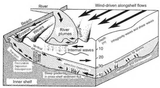
arrow delimiting the size classes of each constituent, from Stramski et al. (2004).. . . . 24 I.3 Conceptual diagram illustrating the major process responsible for sediment transport,
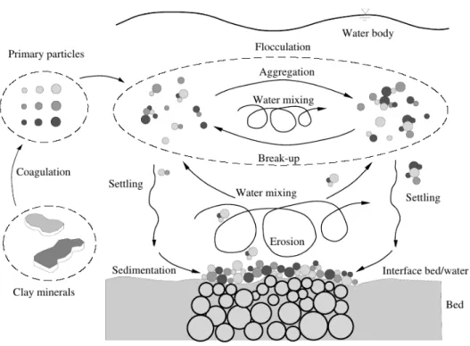
from Nittrouer and Wright (1994).. . . 25 I.4 Conceptual representation of the cohesive fine-sediments cycle within the estuary,
from Maggy (2005). . . 27 I.5 Representation of the SPM granulometric classification (from Many, 2016). . . 27 I.6 Conceptual representation of the formation of micro and macro flocs within an SPM
assemblage (from Montgomery, 1985; Many, 2016). . . 28 I.7 Sketch of the ETM formation by gravitation circulation, adapted from Wolanski and
Gibbs (1995). . . 29 I.8 General scheme of net tidal transport and trapping of suspended sediments in a
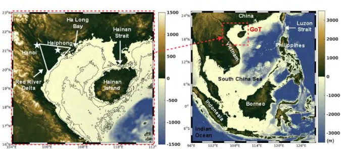
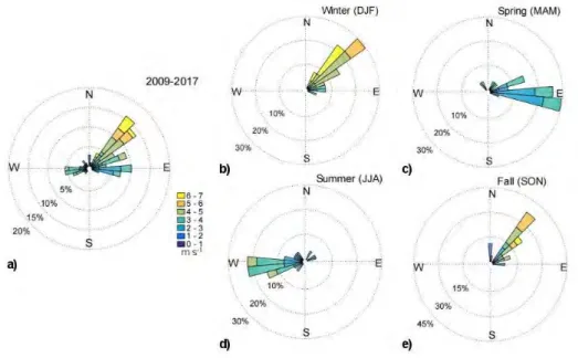
macroti-dal estuary with low density currents (from Allen et al., 1980). . . 29 I.9 Geography of the Gulf of Tonkin and interesting features. . . 32 I.10 Annual (a) and seasonal (b, c, d, e) wind distribution over the GoT from ECMWF over
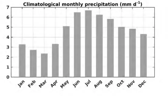
the period 2005-2017.. . . 33 I.11 Climatological monthly precipitation (in mm d-1) over the GoT for the period
2005-2017 from ECMWF. . . 34 I.12 (a) Red River basin catchments (Wei et al., 2019), (b) scheme of the Red River system
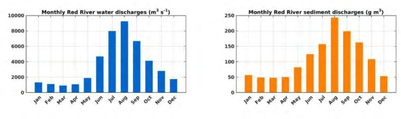
(Vinh et al., 2014). . . 36 I.13 Climatological monthly Red River water (left) and sediment (right) concentration at
Son Tay for the period 1990-2016 from the National Hydro-Meteorological Service. . . 37 I.14 Climatological monthly freshwater discharges for the Lam, Lac Giang, Ma (Vietnam
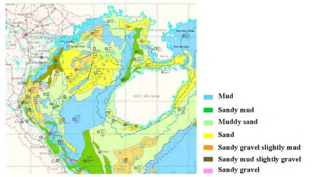
National Hydro-Meteorological Service) Beilun, Qinjiang, Nanliu and Jiuzhou rivers (from the Global Hydroclimatic Data Network, Dettinger and Diaz, 2000). . . 38 I.15 GoT seafloor composition from the Natural Conditions and Environments of Vietnam
Sea and Adjacent Area Altas (2007). . . 39 I.16 Mean SCS surface circulation during (a) summer and (b) winter from Chu et al. (1999). 40 I.17 Schematic patterns of winter circulation in the Gulf of Tonkin from the literature (Gao
et al., 2017). Reference 1 to 4 are given in the text. . . 41 I.18 Schematic patterns of summer circulation in the GoT (from Gao et al., 2017). . . 42 I.19 Tidal amplitude (m) for O1 (a), K1 (b), M2 ( c) and S2 (d) from the tidal atlas FES2014b.. 44 I.20 Spatial distribution of mean seasonal averages (summer, winter) of the wave period
(Tp) (a,d), wave height (Hs) (b, e) and wave energy (c, f ) from Zhou et al. (2014). . . 46 I.21 General pattern of ETM in the Cam-Bach Dang estuary as observed by Vinh et al.
(2018). Blue lines represent isolines (in PSU), turbidity patterns are shown in brown with darker color for higher turbidity values. . . 48 I.22 Morphological changes (mm y-1) in the RRD coastal area from Vinh (2018). . . 49 I.23 Alongshore sediment transport for different cross-sections (x106t) in the RRD coastal
area during dry and rainy season (a) and annually (b), from Vinh (2018). . . 50 vii
II.1 Location of stations ST1, ST2 and ST3 (in red) in the Van Uc River and of Trung Trang and Hon Dau hydrological stations (black star) (Landsat 8 image from September 29,
2017). . . 66
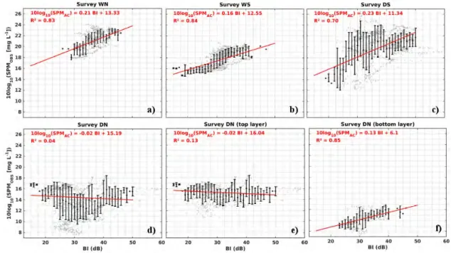
II.2 10log10of suspended matter concentration estimated from CTD OBS (SPMOBSin mg l-1) against the ADCP backscattering index (BI in dB) for each survey WN, WS, DS and DN (panels a, b, c, d respectively). Raw data are shown in grey and the binned data in black, the data trend line is shown in red. Panels e and f correspond to the top and bottom water layers respectively in survey DN. On the y-axis, 10 corresponds to 10 mg l-1, 16 to 40 mg l-1, 20 to 100 mg l-1, 26 to 400 mg l-1. . . 74
II.3 Mean currents directions (in◦N) measured at ST2 during survey DN at high tide (8 am), ebb tide (12 am), low tide (4 pm) and flood tide (2 am). . . 75
II.4 Tidal elevation (in m, black line) and QTT (m3 s-1, blue line), measured QADCP (m3 s-1, red dots) with associated QADCP+ and QADCP- (dark grey and light grey bars, re-spectively), and computed QSED(in t s-1, black dots) with associated QSED+ and QSED -(blue and purple bars, respectively), at all three stations for all four surveys. . . 79
II.5 Simpson parameter values (J m-3) at ST3 (left), ST2 (center) and ST1 (right) for survey WN (orange line), survey WS (cyan line), survey DS (black line) and survey DN (yellow line) during 24h tide cycles. The letters “L" indicates the time of low tide. The missing value at 8pm at ST3 (survey WN) corresponds to a failure in CTD measurement. . . 80
II.6 Salinity (in PSU), N2(in s-2), and turbidity (in FTU) temporal series at ST3, ST2 and ST1 measured in survey DS (a, dry season, spring tides) and in survey DN (b, dry season, neap tides). Note the different colorbars for salinity at ST3 for DS, due to very low values, and between DS and DN for N2and turbidity. . . 81
II.7 a) PSD at each station for all surveys and their associated SPMVC. b) PSD at ST2 in survey DS at high tide (measured at 8 am) and low tide (measured at 8 pm). c) Propor-tions of primary particles, flocculi and microflocs in terms of % of volume occupied, by station and for all four surveys.. . . 84
III.1 (a, left) Gebco bathymetry (in m) and (a, right) details of the Ha Long Bay area (black rectangle in a,left). (b, left) TONKIN_bathymetry data set merged with TONKIN_-shorelines over GoT and (b,right) zoom in the Ha Long Bay area. (c) Absolute (m) and (d) relative (%) differences between TONKIN_bathymetry and Gebco bathymetry (in m). . . 98
III.2 Map of tidal form factor F computed with the amplitudes of tidal waves O1, K1, M2 and S2 obtained from FES2014b-with-assimilation. . . 100
III.3 Shorelines products from OpenStreetSap (blue line), GSHHS (yellow line) and TONKIN_-shorelines (red line) superimposed on a satellite image downloaded from Bing over a small region of the GoT.. . . 103
III.4 Model mesh over the GoT (left) with a zoom in Halong Bay region (right). The maxi-mum refinement (150 m) is reached in the river channels. . . 107
III.5 O1 tidal amplitude (in m) from different products: (a) FES2014b-with-assimilation, (b) FES2014b-without-assimilation, (c) TKN-gebco and (d) TKN. The circle diameter is proportional to the complex error (Appendix ; Eq. III.6 ) between the solutions and satellite altimetry (in m). . . 113
III.6 Same as Fig. III.5 for K1. . . 114
III.7 Same as Fig. III.5 for M2. . . 115
III.8 Same as Fig. III.5 for S2.. . . 116
III.9 Model complex errors (Appendix ; Eq. III.6) relative to altimetry alongtrack data for tests performed with varying the values of the uniform drag coefficient CDover the domain (SET1). The space in between two lines corresponds to the error for each wave. The yellow line therefore corresponds to the cumulative error for all four waves. The red dashed line corresponds to the smallest cumulative error, here equals to 11.50 cm, and obtained for CD=0.9 × 10⁻³m. . . 117
formed with varying the values of the uniform z0over the domain (SET2). The space
in between two lines corresponds to the error for each wave. The yellow line corre-sponds to the cumulative errors for all four waves. The red dashed line correcorre-sponds to the smallest cumulative error, here equals to 10.96 cm, and obtained for z0=1.5 × 10⁻⁵
m. . . 118 III.11 Relative differences (in %) between simulation with CD=f(z0=1.5× 10⁻⁵,H) and
simu-lation with CD=0.9× 10⁻³m compared to FES2014b-with-assimilation (as a reference)
for the tidal harmonics of O1, K1, M2 and S2. . . 120 III.12 Spatial partitioning of the domain for the set of experiment SET3, (a), for SET4 (b) and
for SET5 (c). . . 121 III.13 Model complex errors (Appendix; Eq. 6) relative to altimetry data for tests listed in
Ta-ble 1 performed with non-uniform values of z0(SET3 and SET4). The space in between
two lines corresponds to the errors for each wave. The yellow line corresponds to the cumulative errors for all four waves. The red dashed line corresponds to the smallest cumulative error, found for Test 6 (SET 4), equals to 10.43 cm. . . 122 III.14 Bottom dissipation flux (W m-2) for O1, K1, M2 and S2 computed from model outputs
of simulation “TEST 6”. . . 123 III.15 Relative differences (in %) between simulation TEST6 and simulation with CD=f(z0
=1.5e-5,H) compared to FES2014b-with-assimilation (as a reference) for the tidal harmonics of O1, K1, M2 and S2. . . 124 III.16 RMS* errors (Appendix ; Eq. 6) between numerical simulations (TKN, TKN-gebco,
FES2014b-without-assimilation and FES2014b-with-assimilation) and altimetry data for O1, K1, S2 and M2. . . 126 III.17 RMS* errors (Appendix ; Eq. 6) between numerical simulations (TKN, TKN-gebco,
FES2014b-without-assimilation and FES2014b-with-assimilation) and tide gauges for O1, K1, S2 and M2. . . 127 IV.1 (a) Arakawa C-grid representation: indices, i, j, k refer to grid points in x, y and z
di-rections, respectively, and scalar quantities are represented byφ. (b) σ (sigma) vertical layers coordinates along the red transect. . . 147 IV.2 GoT bathymetry (in m) (a) and details of the Red River system (b). Green dots
corre-spond to rivers represented as a simple grid point in the model, red dots correcorre-spond to rivers of the Red River system represented as channels in the model, the pink line represents the position of the CTD transects and the black stars represent Hon Dau, Bach Long Vy, Son Tay and Trung Trang hydrological stations. . . 153 IV.3 Positions of the HF Radars stations (black dots) overlaid with 20 m depth contours.
The gray and black polygons indicate the coverage boundaries during the summer and winter seasons, respectively (from Roarty et al., 2019).. . . 155 IV.4 Schematic representation of the initial river channels from a top view (a) and from a
lateral view (b). . . 158 IV.5 Tidal amplitude of waves O1 (a) and M2 (b) along the Thai Binh channel grid points
for different values of hc. . . 159
IV.6 Schematic representation of the meshes adjustments made for the Van Uc channel, from a top view (a) and from a lateral view (b). . . 161 IV.7 Tidal amplitude of waves O1 and M2 along the initial Van Uc channel (blue line,
"Chan-nel initial"), the chan"Chan-nel with a real bathymetry (red line, "Chan"Chan-nel real bathy") and the extended channel (yellow line, "Channel extended"). . . 161 IV.8 Comparisons between measurements of water discharges Q at Trung Trang in the
IV.9 Salinity profiles during survey DS (dry season, spring tides) at ST1, ST2 and ST3 (top row) and corresponding salinity profiles from simulation with z0 = 0.01 m (second
row), z0 = 0.001 m (third row), z0 = 0.0001 m (fourth row) and z0 = 0.01 m with
in-creased Van Uc discharges by 10% (last row). . . 163 IV.10 Same as Fig. IV.9 but for survey DN (dry season, neap tides). . . 164 IV.11 Currents velocities (m s-1) measured (a) and modeled (b) at ST2 during survey DN (dry
season, neap tide) at high tide (8 am), ebb tide (12 am), low tide (4 pm) and flood tide (2 am). . . 165 IV.12 Best bottom friction parameterization obtained with T-UGOm in 2D mode. . . 166 IV.13 Tidal amplitudes differences (in m) between the modeled tidal waves and the forcing
tidal waves (FES2014b) for O1 (a,e), K1 (b,f ), M2 (c,g) and S2 (d,h), from SIMU_con-stant_z0(top panels) and from SIMU_varying_z0(bottom panels).. . . 166
IV.14 Evaluation of SIMU seasonal maps of SST. Climatological comparisons of sea surface temperature (SST,◦C) between OSTIA (a, b), SIMU (c, e) and the forcing GOM (c, f ) in summer (top panels) and winter (bottom panels) . . . 168 IV.15 Climatological SST of the summer season (JJA) from simulation without tide. . . 169 IV.16 Evaluations of the monthly SST anomaly signals over the GoT of SIMU and GOM
com-pared to OSTIA (a); of SIMU, GOM and OSTIA comcom-pared to Bach Long Vi hydrological station (b); of SIMU, GOM and OSTIA compared to Hon Dau hydrological station (c). Bias refer to the SST (not anomaly) signal. . . 170 IV.17 Evaluations of the annual (left column) and interannual (right column) SST anomaly
signals over the GoT in SIMU and GOM compared to OSTIA (a, d); in SIMU, GOM and OSTIA compared to Bach Long Vi hydrological station (b, e); in SIMU, GOM and OSTIA compared to Hon Dau hydrological station (c, f ). . . 171 IV.18 Similar to Fig. IV.14 but for sea surface salinity (SSS, PSU) comparison between SMOS,
SIMU and GOM. . . 172 IV.19 Evaluations of the monthly SSS signals over the GoT of SIMU and GOM compared to
SMOS (a); same evaluations but with detrended SSS signals (b). Bias refer to the SSS (not anomaly) signal. . . 173 IV.20 Evaluations of the annual (a) and interannual (b) SSS signals over the GoT of SIMU
and GOM compared to SMOS. . . 174 IV.21 Evaluations of the monthly SSS signals at Hon Dau of SIMU, SIMU+20% and SIMU+40%
compared to in-situ dataset. Bias refer to the SSS (not anomaly) signal. . . 174 IV.22 Evaluations of the annual (a) and interannual (b) SSS signals at Hon Dau of SIMU,
SIMU+20% and SIMU+40% compared to in-situ dataset. . . 175 IV.23 Similar to Fig. IV.14 but for sea level anomaly (SLA, m) comparison between ALTI,
SIMU and the forcing GOM. . . 176 IV.24 Evaluations of the monthly SLA signals over the GoT of SIMU and GOM compared to
ALTI (a), at the annual time-scales (b) and at the interannual time-scales (c).. . . 177 IV.25 Climatological comparisons of SIMU depth-averaged currents (m s-1) (a,b) with schematic
circulation patterns found in literature in summer (top panels) and winter (bottom panels). . . 179 IV.26 Monthly averaged SIMU surface currents intensity fields (in m s-1) overlaid with
cor-responding current directions (arrows) for January, April, July, October and December of 2017 (panels a,b,c,d,e); monthly averaged HF radar-observed surface current inten-sities (in m s-1) and corresponding currents directions for January, April, July, October and December of 2017 (panels f,g,h,i,j). . . 180 IV.27 Temperature (in◦ C) transects along a 25 km across-shore line from SIMU (a,d,g,j),
from CTD observations (b,e,h,k) and biases between SIMU and observations (c,f,i,l). . . 181 IV.28 Same as Fig. IV.27 but for salinity (in PSU). . . 182 IV.29 Winter (a,b,c) and summer (d,c,f ) mean fields of surface Utotal(a,d), UEkman(b,e), Ugeos(c,f )
superimposed with Utotalsurface currents fields (in m s-1) during corresponding
sea-sons. Note that here, summer corresponds to the months of May, June, July and Au-gust, and winter corresponds to the months of October, November, December and January. . . 185 IV.31 Spatial functions (a,b,c,d) and associated principal components (noted PC) of the
tem-poral variability (e) of the first EOF mode on the zonal component of Utotal(a), on the
zonal component of UEkman(b), on the zonal component of Ugeos(c ), and second EOF
mode on the zonal component of Ugeos(d). The product between the spatial and
tem-poral functions denote the intensity of the considered current. On panels b, c, d, R correspond to the correlations between EOF1Utotaland EOF1UEkman,EOF1Ugeosand
EOF2Ugeos, respectively. On panel e, R corresponds the correlation between EOF1Utotal
and EOF1UEkman,R(PC1) corresponds the correlation between EOF1Utotaland EOF1Ugeos,
and R(PC2) to the correlation between EOF1Utotaland EOF2Ugeos. . . 187
IV.32 Same as for Fig. IV.31 for the meridional component of the currents. . . 188 IV.33 Spatial functions (a,b,c,d) and associated principal components of the temporal
vari-ability (e) of the first interannual EOF mode of the zonal component of Utotal(a), of the
zonal component of UEkman(b), of the zonal component of Ugeos(c ), and of the zonal
component of the wind (d). The product between the spatial and temporal functions denote the intensity of the considered current. On panels b, c, d, R correspond to the spatial correlations between EOF1Utotaland EOF1UEkman, EOF1Ugeosand EOF2Ugeos,
respectively. On panel e, R in blue corresponds to the temporal correlation between EOF1Utotal and EOF1UEkman, R in gray corresponds to the temporal correlation
be-tween EOF1Utotaland EOF1Ugeosand R in red corresponds to the temporal correlation
between EOF1UEkmanand EOF1on the zonal wind interannual signal. . . 189
IV.34 Same as Fig. IV.33 but for the meridional component (v) of the currents and the wind. . 190 IV.35 Temporal functions (black lines) on the EOF1 on zonal (a) and meridional (b) wind
components. Overplotted are Niño 4 (solid green lines) and PDO (dotted green lines) indices detrended and filtered with the TY-H13 method.. . . 192 IV.36 March (a), July (b), September (c ) and December (d) monthly mean fields of SSS (in
PSU) superimposed with surface currents monthly mean fields (in m s-1) from SIMU over the period 2009-2017. . . 195 IV.37 Mean summer and winter fluxes (in Sv) through sections 1 to 5 computed from SIMU
over the period 2009-2017 (left), schematic representation of flux dispersal (right). . . . 196 IV.38 Climatological cross-section, rivers and surface fluxes computed for the period
2009-2017. Negative values indicated flux flowing outside the GoT. . . 198 IV.39 Water fluxes (in Sv) in the South China Sea its interocean passages (in blue, adapted
from Fang et al., 2009) and in the GoT (in red, from SIMU). Solid blue lines indicate the cross-sections where fluxes were computed for the Luzon (L), Taiwan (T), Mindoro (MD), Balabac (B), Karimata (K) and Malacca (ML) Straits by Fang et al. (2009). Solid red lines indicate the cross-sections for the Hainan strait (1) and for the total southern boundary of the GoT (2-3), which are computed from SIMU. Arrows denote directions of the mean water transport. Isobaths are in meters.. . . 199 IV.40 Filtered flux signals through sections 1, 2 and 3 (in red) superimposed with EOF1
tem-poral function of the zonal wind (in black). Positive flux values indicate fluxes entering the GoT, negative values indicate fluxes flowing outside the GoT. Note that Section 3 series is reversed. . . 202 IV.41 Typhoon Fabian, Jolina, Paolo and Yolanda trajectories (a) and associated wind when
IV.42 Daily-averaged fluxes (in Sv) generated by typhoons (colored arrows) and monthly accumulated daily-averaged fluxes (grey arrows) for (a) typhoon Fabian and month of June, (b) typhoon Jolina and month of August, (c) typhoon Paolo and month of September, and (d) typhoon Yolanda and month November. Percent values corre-spond to the ratio between typhoon daily fluxes and accumulated fluxes in one month. 204 IV.43 Flux temporal series through sections 2 and 3 for typhoon Fabian, Paolo and Yolanda
and through section 1 and 5 for Jolina, computed for 10 days before and after the pas-sage of the typhoons over the GoT. The convention is again positive (respectively neg-ative) corresponds to input to (respectively output from) the GoT. . . 206 IV.44 Mean wind intensities over the GoT generated by typhoon Parma, Conson, Jolina,
Fabian, Ofel, Paolo, Nesat and Yolanda vs. fluxes through section 3 (in Sv) computed for each typhoon event subtracted of the associated monthly mean flux (stars) and Red line linear regression (red line). R is the correlation coefficient between the fluxes and the typhoon intensities and R² is the coefficient of determination of the regression line. 207 IV.45 Daily mean surface (a, c) and bottom salinity (b, d) (in PSU) from SIMU on September
4th 2017 (a, b) and on December 14th 2017 (c, d). The black solid line represent the isohaline 20 and the locations of sampling stations (ST1, ST2 and ST3) of Chapter II are indicated in red. . . 208 V.1 Schematic representation of the Van Uc estuary during the wet (a, b) and dry season
(c, d) at neap tides (a, c) and spring tides (b, d) as observed during surveys WN (a), WS (b), DN ( c) and DS (d). . . 219 V.2 Schematic patterns of the GoT seasonal circulation under normal (a, d), El Niño (b, e)
and typhoon (c, d) conditions. . . 223 V.3 Boat trajectories and sampling stations of potential future field campaigns in the Van
Uc river’s plume. . . 225 V.4 Monthly mean surface SPM concentrations (g l-1) of August 2009 from satellite
obser-vations (a) and from simulation #1 to #6 (b-g). . . 229 V.5 Monthly mean surface SPM concentrations (g l-1) of August 2009 from simu #7 (a) to
I.1 List of the GoT main tidal constituents. . . 44 II.1 Van Uc surveys characteristics and dates of sampling. Each sampling started at 8 am
and finished at 6 am the following day. . . 67 II.2 Mean water discharges at Trung Trang (QTT), mean water (QADCP) and mean
sedi-ment (QSED) discharges derived from ADCP measurements and determination
coef-ficients (R2), for the four surveys (for our 36 values time series, the 99% significance threshold is reached for a correlation of 0.42). The means are computed over the 3-days period of each survey (36 values), and computed over 24h when showed for each station (12 values). . . 77 III.1 Description of SET 3 and SET 4 (in m).. . . 111 III.2 Mean absolute differences (Appendix ; Eq. III.7) of amplitudes (in cm) and phase (in
deg) of M2, S2, O1, K1 constituents between our reference TKN and satellite altime-try. For comparison, the work of Minh et al. (2014) compared with satellite altimetry and the work Chen et al., (2009) compared to gauge stations are presented. . . 131 IV.1 River lengths as represented in the model of each river of the Red River systems, D
the distance between Son Tay station and the first river grid point and t the time lag imposed to each river discharge. . . 159 IV.2 R, associated significance (p-value), NSE and biases computed for ALTI, SIMU and
GOM at the monthly, annual and interannual time-scales compared to Bach Long Vi and Hon Dau gauges stations.. . . 178 IV.3 Maximum correlation coefficients (at given lags) between EOF1 principal
compo-nents of wind u and v and ENSO, PDO, DMI, SAM and NP indices. All values are significant at 99% confidence level. . . 191 IV.4 Wind behaviors in link with signs of PCs1on Fig. IV.35 and with the seasonal mean
wind. . . 192 IV.5 Water transport (in Sv) through the Hainan strait from previous studies and from our
simulations (negative values indicate an eastward flux). . . 197 IV.6 Correlation coefficients (R) values between the interannual water flux signals through
sections 1, 2, 3 and the temporal functions of the EOF1on zonal and meridional wind.200
A.1 Erosion, deposition and configuration parameters values used in this study. . . 250 A.2 Water column particles characteristics for set-1 and set-2. . . 251 A.3 Proportions (%) of particles in the bottom sediment for different seabed
configura-tions. . . 252 A.4 Summary of sensitivity simulations. . . 252
ADCP: Acoustic Doppler Current Profiler DFR: Delta du Fleuve Rouge
DMI: Dipole Mode Index
DN: survey during the Dry season at Neap tide DS: survey during the Dry season at Spring tide
ECMWF: European Centre for Medium-Range Weather Forecasts EOF: Empirical Orthogonal Function
ENSO: El Niño Southern Oscillation GOM: Global Ocean Model
GdT: Golfe du Tonkin GoT: Gulf of Tonkin
LISST: Laser In situ Scattering and Transmissometry MCM: Mer de Chine Méridionale
MES: Matière En Suspension
NHMS: National Hydro-Meteorological Service NP: Northern Pacific
NTU: Nephelometric Turbidity Unit PDO: Pacific Decadal Oscillation PSD: Particle Size Distribution PSU: Practical Salinity Unit
SAM: Marshall Southern Annular Mode SCS: South China Sea
SLA: Sea Level Anomaly
SOI: Southern Oscillation Index SPM: Suspended Particulate Matter SSC: Suspended Sediment Concentration SSH: Sea Surface Height
SST: Sea Surface Temperature SSS: Sea Surface Salinity TT: Trung Trang
WN: survey during the Wet season at Neap tide WS: survey during the Wet season at Spring tide
Deltas and coastal regions deliver the largest inputs of freshwater and sediments to the shelf and open ocean, understanding water and sediment dynamics and variability in those regions is there-fore crucial. The spatio-temporal variability of estuarine and ocean dynamics under the influence of natural forcings and their impact on sediment transport and fate was assessed along the Red River estuary - coastal ocean - Gulf of Tonkin continuum. First, in-situ estuarine observations evi-denced the seasonal and tidal variabilities of flow and suspended matter, and showed in particular the role of tidal pumping in the estuary siltation. Second, a 3D realistic hydrodynamic model was set up and calibrated with various observations and satellite data. Beforehand, a high-resolution model configuration was implemented and optimized with sensitivity tests of the Gulf of Tonkin’s tidal components to bathymetry and various bottom friction parameterizations. Third, the result-ing optimized configuration was used to study the large scale Gulf of Tonkin circulation at daily, seasonal and interannual scales, and to identify the drivers of their variabilities. Ekman transport variability due to monsoon winds reversal drives the seasonal circulation, which can be reversed in summer by episodic typhoon events and intensified in winter. ENSO, strong typhoon activity and Arctic Oscillation have been identified as drivers of the interannual circulation variability. Lastly, preliminary tests with a sediment transport module coupled with the hydrodynamics model re-vealed the importance of the seabed composition and of the parameterization of the erosion co-efficients.
Keywords : estuarine to regional circulation, sediment transport, variability, in-situ observations,
regional ocean modelling, estuary-coastal ocean continuum, Red River, Gulf of Tonkin
Les deltas et les régions côtières constituent les sources les plus importantes d’eau douce et de matière en suspension vers le plateau continental puis le large, la compréhension de leur dy-namique et de leur variabilité est donc cruciale. Cette thèse vise à mieux comprendre la variabilité spatio-temporelle de la dynamique estuarienne et océanique sous l’influence de forçages naturels et l’influence de cette variabilité sur le transport et devenir des sédiments le long du continuum estuaire - océan côtier du Fleuve Rouge au Golfe du Tonkin. Des observations in-situ collectées dans l’estuaire ont d’abord mis en évidence l’influence de la variabilité saisonnière et de la vari-abilité due à la marée sur le débit et sur le devenir des matières en suspension, en particulier le rôle du pompage tidal dans l’envasement de l’estuaire. Deuxièmement, un modèle hydrody-namique 3D réaliste, basé sur une configuration haute-résolution et un paramétrage optimisés et validés à partir de plusieurs jeux d’observations in-situ et de données satellitaires, a été utilisé pour l’étude de la circulation à l’échelle du Golfe du Tonkin. Cette configuration a préalablement été optimisée à l’aide de tests de sensibilité des solutions de marée à la bathymétrie et à la paramétri-sation du frottement de fond. Les facteurs de la variabilité de cette circulation aux échelles jour-nalière, saisonnière à interannuelle ont été identifiés. La variabilité du transport d’Ekman due à l’inversion saisonnière des vents de mousson a été identifiée comme le principal moteur de la circulation saisonnière, cette dernière pouvant être inversée (intensifiée) en été (hiver) par le passage de typhons. ENSO, l’Oscillation Arctique ou encore une forte activité cyclonique ont été identifiés comme les facteurs de la variabilité interannuelle. Des tests préliminaires avec un mod-ule de transport sédimentaire couplé au modèle hydrodynamique ont révélé l’importance, pour la représentation réaliste du transport de matière en suspension, de la composition du sédiment de fond et du paramétrage des coefficients d’érosion.
Mots clés : circulation estuarienne à régionale, transport sédimentaire, variabilité, observations
in-situ, modélisation océanique régionale, continuum estuaire-océan côtier, Fleuve Rouge, Golfe du Tonkin
General context: understanding the transport and fate of water and matter in the delta-coastal regions continuum, a socio-economic and scientific key question.
Since the start of civilization, humans have settled along rivers, subsequent deltas formed by them and near coastal regions, as the sediments carried along and deposited by flowing rivers created areas rich in nutrients, ideal for agriculture and fishing. Nowadays, deltaic regions hold more than ever ecological and economic values throughout the world. At the transition between water and land, these regions are strategically positioned for trade with the world market, and are major centers of population with intensive agriculture and industry activities (Pont et al., 2002). While these low elevated coastal regions represent only 2% of the earth’s land area (McGranahan et al., 2007), they are home for 10% of the total population (i.e., ∼ 600 million people in 2000; ∼ 650 million in 2050, CIESIN, 2009). In many nations, deltaic and coastal regions are the engines of the national economies with the highest contributions to national GDPs (Gross Domestic Production). For example, the Bengal Delta represents 1.1% of India’s GDP, the Volta Delta, 4.4% of Ghana’s GDP and the Ganges-Brahmaputra-Meghna Delta represents up to 28% of the Bangladesh’s GDP (DECCMA project, 2019). In Vietnam, aquaculture and fisheries in both delta regions (Mekong Delta and Red River Delta) represent 5% of GDP and most of the rice that is worldwide exported (Vietnam is the world’s 2nd rice exporter) is produced in these deltaic regions.
Coastal and delta regions are now considered as "hotspots" in the context of global changes, i.e., as places where high exposure to climate stress and anthropogenic pressure (industrialisation, ur-banisation, resources overexploitation ...) coincides with high levels of vulnerability (IPCC, 2001). Combined to the deltaic subsidence enhanced by local groundwater withdrawal and hydrocarbon and sand extraction, and to the global sea level rise inducing flooding, coastal erosion and saliniza-tion, many deltas and surroundings have moved from a condition of active growth to a destructive
phase (Milliman et al., 1989; Poulos and Collins, 2002; Day et al., 1995). Giosan et al. (2014) fur-ther showed that sediment input to most major deltas is insufficient to maintain elevation with rising sea level. Coastal systems and low-lying areas will increasingly experience sea level rise and associated phenomena throughout the 21st century and beyond (IPCC, 2014). Economically, cli-mate change has the potential to impact the deltas by reducing the GBP per capita by 8.5 to 14.5% , through impacts on infrastructures, agriculture and fisheries (DECCMA project, 2019).
Deltas and coastal oceanic regions are not only key interfaces between the land and the ocean, transferring huge quantities of water, organic and inorganic matter of natural and anthropogenic origins between those two compartments of our planet system. They also represent preferential concentration areas for land-derived material (as sediments, dissolved and particulate nutrients), which play a main role in the sequestration of chemical elements (carbon, nitrogen, pollutants) and in the sedimentary budget of the continental margins. The richness of those areas in terms of matter availability explains their high biodiversity. Indeed, coastal zones sustain sensitive ecosys-tems, provide critical habitat for many endangered species and are often classified as public her-itage (Ramesh et al., 2015). Considering the East Asian Seas, the coastal regions are hosts for 35% of the world’s mangrove, 33% of the world’s seagrass bed and 33% of the world’s coral reef (Daily Bulletin EAS Congress, 2018). Globally, coastal ocean represents 15% of the global oceanic primary production, 47% of the global annual export of particulate organic carbon, 90% of the sedimen-tary mineralization and 75-90% of the oceanic sink of suspended load (Jahnke, 2010; Simpsons and Sharples, 2012).
A better understanding of the functioning, variability and evolution of deltas and coastal regions in terms of water and matter transport and fate is therefore of high socio-economic and scientific importance.
To address these issues, the response of the scientific community is organized on the basis of the LOICZ (Land-Ocean Interaction in the Coastal Zone), which federates global scientific or-ganizations around common objectives of addressing the issue of the actual responses of the coastal ocean to anthropogenic and climatic forcings (Ramesh et al., 2015). One of the funda-mental approach of this project was to recognize the coastal zone as a global compartment rather than a geographical boundary of interaction between the land and sea. Indeed, the riverine and oceanic shelf processes were often considered separately, with hydrologists on one side and phys-ical oceanographers on the other. However, understanding the complex connexions of deltaic and
plinary studies, which connect hydrology, oceanography, atmospheric and soil sciences, but also geology, chemistry, biology and ecology.
The study of delta and coastal regions is therefore not only a scientific challenge, but also a method-ological challenge, requiring the connection and coupling of existing tools and methods from dif-ferent scientific disciplines, and the development of new ones. For example, since estuarine and coastal processes are very fine processes at the scale of the global ocean, studies based on numer-ical tools imply to increase regional model resolution and to use grid meshes that can adapt to the fine river/coastal geography and bathymetry. In addition, forcing field data (continental, atmo-spheric and oceanic) as well as bathymetry data are key ingredients for those numerical studies and constitute a real stake for the scientific community as they require high temporal and spa-tial resolutions and are often difficult to access, for physical or political reasons. Furthermore, due to the different regions locations and to associated external forcings, the characteristics and processes largely vary from one region to another. Therefore, dedicated in-situ observations cam-paigns for each case study are needed and are a prerequisite for understanding and studying their specific processes and variabilities. Such observations are however often few and far between, and can constitute a real acquisition challenge for scientists.
Case study: the Red River Delta and Gulf of Tonkin system
The Red River Delta (RRD), located in the western coast of the Gulf of Tonkin (GoT) in the South China Sea (SCS), is an ideal case study for those questions since it gathers most of the issues de-scribed above. It has one of the highest demographic densities in the world (>1000 inhab km-2), gathering highly populated rural areas and big urban centers in very low elevated areas (<10 m): Hanoi (7.6 M) and Haiphong (2.4 M) (from the Statistical Yearbook of Vietnam, 2017). The Red River is the principal source of freshwater (3500 m3s-1) and sediments (40 Mt y-1) to the GoT. In terms of delta plain surface, the RRD is the fourth largest delta in Southeast Asia after the Mekong, Irrawaddy and Chao Praya deltas. The RRD is fertile, with approximately 47% of its superficy used for agriculture or aquaculture, and it constitutes 56% of the country’s rice production (General Statistics Office, 1996-2006). This region is also a key to the economy of Vietnam, with the capital city of Hanoi, with Ha Long Bay (a UNESCO world heritage site) for its particular touristic value and with the Hai Phong ports system which connects the north of Vietnam to the world market. This latter is the second biggest harbour of Vietnam with a particular fast-growing rate in terms
of volume of cargos passing through, of about 4.5x10⁶to 36.3x10⁶tons from 1995 to 2016, respec-tively (Statistical Yearbook of Vietnam, 2017).
The RRD and GoT system constitutes an estuarine, coastal and marine environment that is sub-mitted to a large range of influences of several origins (atmospheric, oceanic, continental and an-thropogenic) and scales (from daily to decadal and climate change). The atmospheric variability is associated to typhoons, drought and flooding, seasonal monsoon, interannual ENSO oscilla-tion and long term climate change. The oceanic influence on the RRD and GoT system resembles storm surges, wave and tidal forcing and large scale circulation (Wyrtki, 1961). The RRD-GoT sys-tems is furthermore submitted to continental fluxes of freshwater and associated matter from the Red River watershed and rivers. In addition, anthropogenic pressures impact the system, such as the pollution due to activities associated to a galloping economic, groundwater and surface water pumping, dams and sand dredging (Le et al., 2007). The Red River delta and surroundings regions are therefore threatened by many natural and anthropogenic hazards. For example, sea level has risen by 20 cm over the past 50 years, and a 1 m rise is planned for 2100, potentially resulting in the salinization of 30 to 50% of the RRD (Duc et al, 2012). The illegal release of 300 tons of toxic waste water from the Formosa plan killed marine life along almost 200 km of the GoT coast in April 2016 and more than 100 tons of dead fishes were washed up on the shores, resulting in a $ 5 M loss for local fishermen, a 30% decrease of tourists’ visits, not to mention the unevaluated indirect economic and health impacts. This last event moreover revealed the strong lack of ma-rine and coastal pollution monitoring (from in-situ measurements to operational modeling and satellite image exploitation), management and mitigation in this region.
In this context, it is fundamental to improve the understanding of the response of Red River - GoT continuum waters and sediment load, from the watershed to coastal and marine environments, to those different forcing factors, and to develop tools and expertise for the applied and operational management and monitoring of this environment. For example, since pollutants (such as dis-solved metals and pathogens) can attach to the riverine suspended sediments, understanding sed-iment spread and fate in the coastal area would be a great asset in monitoring catastrophic events such as the Formosa one. This need has been formally identified by the Vietnamese government and clearly appears in the objectives of « The Strategy for Science and Technology Development for the 2011-2020 period » document published by the Ministry of Science and Technology.
estuary-coastal-open sea continuum in terms of transport and fate of water and sediments taking the case study of the Red River Delta - GoT system. First, the focus is made on understanding the hydrodynamics and identifying the drivers of its variability, from the Red River to the GoT. The second step consists in understanding how the hydrodynamics and associated variability com-bined to the sedimentary processes along the continuum influence the fate of suspended matter. For that, specific methodologies were developed, with field campaigns dedicated to the analysis of the seasonal and tidal variability of estuarine parameters (hydrodynamics and sediment fate), and with high-resolution models implemented for the first time over the region.
This manuscript is organized around 5 chapters. The first chapter presents the scientific and re-gional contexts of this thesis, reviewing the existing knowledge on hydro-sedimentary dynamics in macrotidal systems in general and on characteristics and specificities of the RRD-GoT system. Methodologies developed and results obtained during this Ph.D. are presented in the next three chapters (Chapter II, III and IV). Chapter II explores the variability of estuarine hydro-sedimentary dynamics, based on in-situ observations in the Red River estuary at tidal and seasonal scales. Chapter III focuses on the tidal representation over the Gulf of Tonkin in numerical models using a 2D unstructured grid numerical model. Chapter IV describes the circulation and fluxes variability of the GoT at daily, seasonal and interannual scales, based on 3D numerical simulations presented and evaluated in the same chapter.
Finally, Chapter V gives the conclusions and discusses preliminary results on sediment transport along the RRD, and proposes perspectives for future work.
References
• CIESIN (Center for International Earth System Science Information Network) (2009) Low-elevation coastal zone (LECZ) urban-rural estimates. Global Rural-Urban Map-ping Project (GRUMP), Alpha Version, Pallisades, NY; Socioeconomic Data and Appli-cations Center (SEDAC), Columbia Univsersity, http://sedac.ciesin.columbia.edu/ data/collection/lecz
• Day J. W., Pont D., Hensel P. F., Ibanez C. (1995) Impacts of sea-level rise on deltas in the Gulf of Mexico and the Mediterranean: the importance of pulsing events to sustainability, Estuaries, 18: 636-647,https://doi.org/10.2307/1352382.
• Daily Bulletin East Asia Seas Congress (2018) Iloilo Convention Center, Philippines; 27-30 November 2018. Available at http://eascongress2018.pemsea.org/wp-content/ uploads/2018/11/EASC2018-Daily-Bulletin-Day-2-2.pdf
• Deltas, vulnerability and Climate Change; Migration as an Adaptation (DECCMA): Climate change and the economic future of deltas in Africa and Asia: Policy brief, 2019.
• Duc Nguyen, Umeyama M., Shintani T. (2012) Importance of geometric characteris-tics for salinity distribution in convergent estuaries, J. Hydrol., 448-449, 1-13, doi: 10.1016/j.jhydrol.2011.10.044.
• General Statistics Office: Statistical Yearbook of Vietnam 2017, Statistical Publish-ing House: Hanoi, Vietnam, http://www.gso.gov.vn/default_en.aspxtabid=515& idmid=5&ItemID=18941, 2017.
• Giosan L., Syvitski J. P. M., Constantinescu S., Day J. (2014) Protect the world’s deltas, Nature, 516, 31-33, doi: 10.1038/516031a.
• IPCC (2001) Climate change 2001: impacts, adaptation and vulnerability. Tech. rep., Inter-governmental Panel on Climate Change.
• IPCC (2014) Climate change 2014: Synthesis report summary for policymakers,https:// www.ipcc.ch/site/assets/uploads/2018/02/AR5_SYR_FINAL_SPM.pdf.
• Jahnke R. A. (2010) Global synthesis. Carbon and Nutrient Fluxes in Continental Margins: A Global Synthesis. Liu K. K., Atkinson L., Quinones R. A., Talaue-McManus L., Berlin Heidel-berg, Springer-Verlag, 597-615. Le, T. P. Q.,Garnier J., Billen G., Théry S., Chau V. M. (2007) The changing flow regime and sediment load of the Red River, Viet Nam. J. Hydrol. 334: 199-214, doi:10.1016/j.jhydrol.2006.10.020
• McGranahan G., Balk D., Anderson B. (2007) The rising tide: assessing the risks of climate change and human settlements in low-elevation coastal zones. Environ. Urbanization 19(1), 17-37, doi: 10.1177/0956247807076960.
• Milliman J. D., Broadus J. M., Gable F. (1989) Environmental and economic implications of rising sea-level and subsiding deltas: the Nile and Bengal examples, Ambio, 18(6), 340-345. • Pont D., Day J. W., Hensel P., Fanquet E., Torre F., Rioual P., Ibanez C., Coulet E. (2002)
Response scenarios for the deltaic plain of the Rhone in the face of an accelerated rate of sea-level rise with special attention to Salicornia-type environments, Estuaries, 25, 337-358,
https://doi.org/10.1007/BF02695978.
• Poulos S. E., Collins M. B. (2002) Fluviate sediment fluxes to the Mediterranean Sea: a quan-titative approach and the influence of dams. In: Jones S. J., Frostick L. E. (ed.), Sediment Flux to Basins: Causes, Controls and Consequences. Special Publications, 191. Geological Society, London, pp. 227-245.
• Ramesh R., Chen Z., Cummins V., Day J., D’Ellia C., Dennison B., Forbes D. L., et al., (2015) Land-Ocean interactions in the Coastal Zone: Past, present & future, Anthropocene 12, 85-98, doi: 10.1016/j.ancene.2016.01.005/
• Simpson J. H., Sharples J. (2012) Introduction to the physical and biological oceanography of shelf seas. Cambridge University Press.
Contexte général : comprendre le transport et le devenir de l’eau et de la matière dans le con-tinuum delta-océan côtier, une question socio-économiquement et scientifiquement clé.
Dès les débuts de la civilisation, attiré par la fertilité des terres et des eaux riches en nutriments apportés par les rivières, l’Homme s’est préférentiellement installé le long des cours d’eau, des deltas et des zones côtières. De nos jours, les régions deltaïques sont, et plus que jamais, par-ticulièrement précieuses pour l’écologie et l’économie mondiale. Stratégiquement positionnées à la transition entre la terre et la mer, ces régions regroupent d’intenses activités agricoles, in-dustrielles et commerciales avec le monde, et abritent de grands centres de population (Pont et al., 2002). En effet et bien que ces régions côtières de faibles altitudes ne représentent que 2% de la superficie terrestre (McGranahan et al., 2007), elles abritent jusqu’à 10% de la population totale (soit 600 millions de personnes en 2000 et jusqu’à 650 millions en 2050, CIESIN, 2009). Dans de nombreux pays, les régions deltaïques et côtières sont les moteurs des économies na-tionales et contribuent largement au PIB (Production Intérieure Brute). Par exemple, le delta du Bengale représente 1,1% du PIB de l’Inde, le delta de la Volta, 4,4% du PIB du Ghana et le delta du Gange-Brahmapoutre-Meghna représente jusqu’à 28% du PIB du Bangladesh (projet DECCMA, 2019). Au Vietnam, les activités aquacoles et piscicoles des régions deltaïques (delta du Mékong et delta du Fleuve Rouge) représentent au total 5% du PIB. De plus, la majeure partie du riz exporté dans le monde est produite dans ces régions deltaïques, le Vietnam étant le deuxième exportateur mondial de riz. Le Groupe d’experts intergouvernemental sur l’evolution du climat a classifié les régions côtières et deltaïques comme des "points chauds" dans le contexte du changement clima-tique global, c’est-à-dire comme zones où une forte exposition au stress climaclima-tique coïncide avec des niveaux élevés de vulnérabilité (rapport du GIEC, 2001). Au cours des dernières décennies, de nombreux deltas et régions côtières associées sont passés de conditions de croissance active à des conditions de décroissance, causées par l’affaissement deltaïque qui est lui-même accentué par
les actions combinées de prélèvements locaux d’eau souterraine et l’extraction d’hydrocarbures et par l’élévation du niveau de la mer à l’échelle mondiale qui induit inondations, érosions des zones côtières et salinisation des terres (Milliman et al., 1989 ; Poulos et Collins, 2002 ; Day et al., 1995). Giosan et al. (2014) ont en outre montré que l’apport de sédiments dans la plupart des plus gros deltas mondiaux est insuffisant pour maintenir l’élévation de ces deltas face à la montée du niveau de la mer, qui au cours du 21e siècle et au delà, devrait continuer d’augmenter (GIEC, 2014). Sur le plan économique, il a été estimé que les répercussions du changement climatique sur les in-frastructures et sur les activités agricoles et piscicoles des zones deltaïques et côtières pourraient réduire le PIB par habitant de 8,5 à 14,5% (projet DECCMA, 2019).
Les deltas et les régions océaniques côtières sont des interfaces clés entre la terre et l’océan, qui transfèrent d’énormes quantités d’eau, de matière organique et inorganique d’origine naturelle et anthropiques entre ces deux compartiments. Elles représentent également des zones préféren-tielle pour l’accumulation de matériaux d’origine terrestre (sédiments, nutriments dissous et par-ticulaires), qui jouent un rôle essentiel dans la séquestration des éléments chimiques (carbone, azote, polluants) et dans le bilan sédimentaire des marges continentales. La richesse de ces zones en termes de disponibilité de matière, liée à cette situation d’interface clé, explique la grande bio-diversité et la richesse des écosystèmes qui y sont rencontrés. En effet, les zones côtières peu-vent abriter des écosystèmes sensibles et fournir des habitats essentiels à de nombreuses espèces menacées, et sont souvent classées comme patrimoine public commun (Ramesh et al., 2015). Les régions côtières des mers d’Asie de l’Est abritent 35% des mangroves, 33% des herbiers marins et 33% des récifs coralliens mondiaux (Daily Bulletin EAS Congress, 2018). De plus, il a été es-timé que l’océan côtier global représente 15% de la production primaire océanique mondiale, 47% de l’exportation annuelle mondiale de carbone organique particulaire, 90% de la minéralisation sédimentaire et représente 75 à 90% du puits océanique de matière en suspension (Jahnke, 2010 ; Simpsons and Sharples, 2012).
Une meilleure compréhension du fonctionnement, de la variabilité et de l’évolution des deltas et des régions côtières, en termes de devenir de l’eau et de la matière, est donc socio-économiquement et scientifiquement primordiale. Pour répondre à ces questions, la communauté scientifique s’est organisée autour du projet LOICZ (Land-Ocean Interaction in the Coastal Zone), qui fédère des organisations scientifiques mondiales autour d’objectifs communs pour comprendre les réponses de l’océan côtier face aux forçages anthropiques et climatiques (Ramesh et al, 2015). L’une des ap-proches fondamentales de ce projet est de reconnaître la zone côtière comme un compartiment tel
et océaniques sont en effet souvent considérés séparément avec les hydrologues d’un côté et les océanographes de l’autre. Il n’est cependant pas possible de comprendre les liens complexes entre les régions deltaïques et côtières avec des approches par secteur; il faut au contraire considérer des études interdisciplinaires qui relient l’hydrologie, l’océanographie, les sciences atmosphériques ainsi que la géologie, la chimie, la biologie et l’écologie. L’étude des deltas et des régions côtières n’est donc pas seulement un défi scientifique, mais aussi un défi méthodologique, qui exige la connexion et le couplage d’outils et méthodes issus de différentes disciplines scientifiques ainsi que le développement de nouveaux outils. Par exemple, les processus estuariens et côtiers sont des processus à très fines échelles comparés aux processus de l’océan global. Il est donc néces-saire d’adapter et d’augmenter la résolution des modèles numériques régionaux et d’utiliser des maillages de grille qui peuvent suivre les détails de la géographie et bathymétrie des rivières et des côtes, ce qui peut entraîner des coûts informatiques élevés. De plus, les champs forçants (con-tinentaux, atmosphériques et océaniques) ainsi que les données bathymétriques constituent un véritable enjeu pour la communauté scientifique car ils nécessitent des résolutions temporelles et spatiales élevées et sont souvent difficiles d’accès, pour des raisons physiques et/ou politiques. De plus, en raison de l’emplacement des différentes régions et des forçages externes associés, les caractéristiques et les processus varient largement d’une région à l’autre. C’est pourquoi des cam-pagnes d’observation in-situ dédiées à chaque site sont nécessaires et constituent une condition nécessaire et préalable à la compréhension et à l’étude de la variabilité des processus. Cepen-dant, ces observations sont souvent peu nombreuses et éloignées les unes des autres et peuvent constituer un véritable défi d’acquisition pour les scientifiques.
Étude de cas : le système Delta du Fleuve Rouge Golfe du Tonkin
Le Delta du Fleuve Rouge (DFR), situé sur la côte ouest du Golfe du Tonkin (GdT) en Mer de Chine Méridionale (MCM), est un cas idéal pour étudier ces questions puisqu’il recense la plupart des problèmes décrits ci-dessus. Cette région possède l’une des densités démographiques les plus élevées du monde (>1000 hab km²), regroupant des zones rurales très peuplées et de grands cen-tres urbains dans des zones de très faibles altitudes (<10 m) : Hanoï (7,6 M) et Haiphong (2,4 M) (Statistical Yearbook of Vietnam, 2017). Le Fleuve Rouge constitue la principale source d’apports d’eau douce (3 500 m3s-1) et de sédiments (40 Mt y-1) pour le GdT. En termes de surface, le delta est le quatrième plus grand delta d’Asie du Sud-Est après les deltas du Mékong, de l’Irrawaddy et du Chao Praya. Il est également très fertile, avec environ 47% de sa superficie utilisée pour
l’agriculture et l’aquaculture, et il représente 56% de la production rizicole du pays (General Statis-tics Office, 1996-2006). Cette région est également clé pour l’économie vietnamienne, grâce à sa capitale Hanoï, à la baie d’Ha Long (patrimoine mondial de l’UNESCO) qui attire de nombreux touristes et grâce au port d’Hai Phong qui permet de relier le nord du Vietnam au commerce mon-dial. Ce dernier est le deuxième plus grand port du Vietnam avec un taux croissant de volume de cargaisons transitant par le port, particulièrement rapide, avec une augmentation de 4,5x10⁶à 36,3x10⁶tonnes de 1995 à 2016, respectivement (Statistical Yearbook of Vietnam, 2017).
Le système DFR et GdT est donc composé de milieux estuariens, côtiers et océaniques soumis à un large éventail d’influences qui ont plusieurs origines (atmosphérique, océanique, continentale et anthropique) et plusieurs échelles (du journalier au décennal et au changement climatique). Les typhons, les sécheresses, les inondations, les moussons, l’oscillation ENSO et le changement climatique à long terme composent la variabilité atmosphérique.
L’influence océanique sur le système DFR et GdT correspond aux forçages par la marée, par la cir-culation grande échelle et celle impactée par les tempêtes (Wyrtki, 1961). Le système DFR-GdT est également soumis aux flux continentaux d’eau douce et de matières associées (sédiments, nu-triments, matières organiques, polluants) qui proviennent du bassin versant et des rivières, et à l’influence météorologique naturelle. Les activités anthropiques impactent aussi le système, comme par exemple la pollution due aux économies croissantes, le pompage des eaux souter-raines et de surface, les barrages qui perturbent les cours d’eau et les dragages de sable (Le et al., 2007). Le DFR et ses régions environnantes sont donc menacés par de nombreuses pressions na-turelles et anthropiques. Par exemple, le niveau de la mer a augmenté de 20 cm au cours des 50 dernières années et une élévation de 1 m est prévue pour 2100, ce qui pourrait entraîner la salini-sation de 30 à 50% du DFR (Duc et al, 2012). De plus, le déversement illégal de 300 tonnes d’eaux usées toxiques de l’usine Formosa en Avril 2016 a anéanti la vie marine le long de 200 km de la côte du Golfe, et plus de 100 tonnes de poissons morts ont été rejetés sur les côtes, entraînant une perte de 5 M$ pour les pêcheurs locaux, une diminution de 30% des visites touristiques, sans parler des impacts économiques et sanitaires indirects qui n’ont pas été évalués. Ce dernier événement a d’ailleurs révélé un manque de surveillance de la zone marine et côtière (absence de mesures in situ, de modélisation opérationnelle et d’exploitation d’images satellites) ainsi qu’un manque de gestion de la catastrophe.
charge sédimentaire, depuis le bassin versant vers les milieux côtiers et océaniques, et de dévelop-per des outils et exdévelop-pertises pour la gestion appliquée et opérationnelle, et pour la surveillance de ce milieu. Comme les polluants (tels que les métaux dissous et les agents pathogènes) peuvent, par exemple, se fixer aux sédiments en suspension présents dans les rivières, il est très utile de comprendre la dispersion et le devenir de ces sédiments dans la zone côtière afin de surveiller des catastrophes telles que celle de l’usine Formosa. Ce besoin a été formellement identifié par le gouvernement vietnamien et apparaît clairement dans les objectifs du document " Stratégie de développement scientifique et technologique pour la période 2011-2020 " publié par le Ministère de la Science et de la Technologie.
Les objectifs de la thèse
L’objectif scientifique général de cette thèse est de contribuer à améliorer la compréhension du continuum estuaire-côte-océan en termes de transport et de devenir de l’eau et des sédiments apportés par les fleuves des régions deltaïques, en prenant le cas du système DFR-GdT. Première-ment, l’accent est mis sur la compréhension de l’hydrodynamique et sur l’identification des fac-teurs de sa variabilité, depuis le Fleuve Rouge vers le GdT. La deuxième étape consiste à compren-dre comment l’hydrodynamique et la variabilité associée, combinées aux processus sédimentaires le long du continuum, peuvent influencer le devenir de la matière en suspension. Ces étapes sont réalisées à l’aide de méthodologies spécialement développées pour cette étude, de campagnes de terrain dédiées à l’analyse de la variabilité saisonnière et marémotrice sur des paramètres estu-ariens (hydrodynamique et devenir des sédiments), et de modèles haute-résolution implémentés pour la première fois dans la région qui sont combinés à des forçages précis.
Ce manuscrit s’articule autour de cinq chapitres. Le premier chapitre présente les contextes sci-entifiques et régionaux de cette thèse, passant en revue les connaissances existantes sur la dy-namique hydro-sédimentaire dans d’autres systèmes macrotidaux et sur les caractéristiques et spécificités du système DFR-GdT. Les méthodologies développées et les résultats obtenus au cours de cette thèse sont présentés dans les trois chapitres suivants (chapitres II, III et IV). Le Chapitre II explore la variabilité de la dynamique hydro-sédimentaire estuarienne, à partir d’observations in-situ dans l’estuaire du Fleuve Rouge aux échelles de la marée et des saisons. Le chapitre III porte sur la représentation des principales composantes de la marée du GdT dans des modèles numériques, en utilisant un ensemble de données bathymétriques à haute résolution et une
paramétri-sation ajustée du frottement du fond. Le chapitre IV décrit la variabilité de la circulation et des flux dans le GdT aux échelles journalières, saisonnières et interannuelles, sur la base de simulations numériques 3D présentées et évaluées dans ce même chapitre.
Enfin, le chapitre V présente les conclusions de cette thèse et discute de résultats préliminaires sur le transport sédimentaire le long du delta, et propose des perspectives de travaux futurs.
Introduction
Contents
I.1 Complexity of hydrosedimentary processes along the estuary coastal ocean -open ocean continuum . . . . 22
I.1.1 Continental processes . . . 22 I.1.2 Coastal processes . . . 23 I.1.2.1 SPM fate on ocean margins . . . 23 I.1.3 Transition zone between continental and marine waters: estuarine
pro-cesses . . . 26 I.1.3.1 Cycle of fine sediments within the estuary . . . 26 I.1.3.2 Fine sediment aggregation . . . 27 I.1.3.3 Estuarine turbidity maximum . . . 28 I.1.3.4 Influence of anthropogenic activities . . . 30
I.2 Regional settings and scientific questions in our study area : the Red River Delta to Gulf of Tonkin system . . . . 31
I.2.1 General description of the Gulf of Tonkin . . . 31 I.2.1.1 Geography. . . 31 I.2.1.2 RRD geology . . . 31 I.2.1.3 Climate . . . 33 I.2.1.4 River influences . . . 35 I.2.1.5 Seabed, tidal flats and river-bed sediments . . . 37 I.2.2 Hydrodynamical conditions of the GoT . . . 40 I.2.2.1 General circulation. . . 40 I.2.2.2 Tides . . . 43 I.2.2.3 Waves . . . 45 I.2.3 Hydrological and SPM dynamics in the estuarine and coastal area . . . 47 I.2.3.1 Estuarine processes . . . 47 I.2.3.2 Coastal morphodynamics and sediment transport along the RRD 48
I.3 Objectives and thesis outlines. . . . 50
I.4 References . . . . 52