Comparative analysis between analytical
approximations and numerical solutions
describing recession flow in unconfined
hillslope aquifers
David Rocha1, Jan Feyen2 and Alain Dassargues1,3
1PhD student, Hydrogeology and Engineering Geology Group, Department of Geology-Geography, Katholieke Universiteit Leuven, Celestijnenlaan 200 E, 3001 Leuven (Heverlee), Belgium ([email protected])
Phone: +32-16-326449 Fax: +32-16-326401
2 Division Soil and Water, Department of Land Management and Economics,
Katholieke Universiteit Leuven, Heverlee, Belgium ([email protected])
3 Hydrogeology, Department of Georesources, Geotechnologies and Building
Materials, Université de Liège, Liège, Belgium ([email protected])
Abstract Recession flow of aquifers from a hillslope can be described by the non-linear Boussinesq equation. Under strong assumptions and for specific conceptual formulations, Boussinesq and others, obtained analytical approximations or linearized versions to this partial differential equation. A comparative analysis between analytical approximations of the Boussinesq equation and numerical solution of the receding flow of an unconfined homogeneous aquifer (horizontal, inclined and concave aquifer floor) was carried out. The objective was to
define the range where the analytical solutions approximate the numerical solution. The latter was considered in this study as the reference method, because it requires less simplifying assumptions. Results showed that recession flows obtained with the considered analytical approximations yield similar values only for certain ranges of aquifer properties and geometries.
Keywords Boussinesq equation, groundwater flow, analytical approximations,
numerical solutions, numerical modeling
Introduction
Boussinesq (1877) was among the first researchers to conduct theoretical work on recession hydrographs, more in particular on spring flowrates. Under strong assumptions, he found that the outflow from an aquifer with a concave floor had the form Ce-αt, with C being an arbitrary value depending on the initial conditions and α (generally known as recession coefficient) a positive constant dependent of the geometric configuration of the aquifer and its hydraulic conductivity. During the years, exponential decay relationships of the same type Q ~ e-αt were derived by Maillet (1905), Horton (1933), Nathan and McMahon (1990), Vogel and Kroll (1992), Brutsaert (1994), Shevenell (1996), Long and Derickson (1999), among others. Different approximations have also been proposed considering inclined aquifer floor, as proposed by Boussinesq (see Eq. 2). For example, when the slope angle, i, of the aquifer bottom is large, the kinematic wave approach becomes applicable (Henderson and Wooding, 1964; Beven, 1981; Troch et al., 2002), since under this approximation the second-order diffusive term disappears. In the latter case the hydraulic gradient is assumed to be equal to the bed slope,
For horizontal aquifer floors, i=0, several analytical solutions are known. Among them, two relevant equations exist the short-time and long-time solution, respectively. Polubarinova-Kochina (1962) developed the short-time solution applicable to a fully penetrating stream draining an initially saturated aquifer, said to be valid before the water table reaches the upward corner of the considered aquifer at x=B (Fig.1). Of particular interest in the present study is the long-time Boussinesq exact analytical solution.
Based on simplifying assumptions, Boussinesq (1904) obtained a solution assuming an inverse incomplete beta function as the initial condition for the groundwater table. Its outflow is characterized by non-linear behaviour (quadratic form), said to be valid after large t, when the water table height at x=B is smaller than the aquifer depth D (Fig.1), and the water table profile resembles the assumed shape of the inverse incomplete beta function. In contrast to the exponential decay relationships, where the recession coefficient α is constant, the performance of the previously described short and long-time solutions, is sensitive to the choice or definition of t=0 in the hydrograph Q=Q(t). It is practically impossible to determine in any consistent way the beginning of the recession from a continuous river flow record with intermittent dry and wet periods. To avoid this difficulty Brutsaert and Nieber (1977) proposed to analyze the hydrograph in a differential form, meaning the elimination of the uncertainty involved in the determination of a consistent time reference. Brutsaert and Nieber (1977) presented two equations of the form dQ/dt=-aQb, one valid for small t with slope
b1=3, and the other valid for large t with slope b2=3/2. Each equation, when plotted in a log-log diagram defines two lines. The intercept of these two lines, which according to Brutsaert and Nieber (1977), solely depends on the hydraulic
and geomorphologic characteristics of the basin, would define the situation where it is assumed that the aquifers start to behave in accordance with the solution of large t. Brutsaert and Nieber (1977) low flow analysis has been extensively applied (Troch et al., 1993; Brutsaert and Lopez, 1998; Szilagyi et al., 1998; Parlange et al., 2001; Mendoza et al., 2003; Rupp and Selker, 2005; among others). In order to find a unifying theory that explains both short-time and long-time behaviours, Parlange et al. (2001) provided a single analytical formulation that gives a smooth transition between the two flow regimes. However, the application of the method is fundamentally linked to the Brutsaert and Nieber (1977) solution, since it requires that the data to be analyzed show a slope of 3 for the short time and 3/2 for the long-time formulation.
Brutsaert (1994) derived for the groundwater flow equation in a sloping aquifer, Equation 2, an analytical solution assuming h=pD, p being a constant to compensate for the approximation resulting from the linearization. In this way he obtained the outflow rate when draining from a complete saturation of the hillslope aquifer. Even though his solution may be applied for a broad range of slope angles, i, applications in sloping conditions are still said to be subject for further research. In his paper Brutsaert (1994), also presented an equation for the case of i=0, which is quite similar to the Boussinesq (1877) equation for the case of a concave aquifer floor. Currently, different researchers are developing alternative analytical approximations for computing baseflow to rivers and hillslope groundwater flows (Serrano and Workman, 1998; Verhoest and Troch, 2000; Troch et al., 2002; Troch et al., 2003; Rupp and Selker, 2005; among others). Parallel to this evolution, numerical models are increasingly used for analyzing groundwater flow and for assessing the efficiency of the different
proposed analytical solutions (Szilagy et al., 1998; Dewandel et al., 2003; Paniconi et al., 2003; Troch et al., 2003; Basha and Maalouf, 2005; Huyck et al., 2005; Pulido-Velazquez et al., 2006; among others). Wittemberg (1999) even suggests that to better describe the groundwater component of a basin or hillslope the use of numerical models should be encouraged. Whereas some of the numerical assessments or comparisons with numerical models of Boussinesq approximations include a sensitivity or uncertainty analysis to the soil hydraulic properties (i.e., Dewandel et al., 2003; Troch et al., 2004; Huyck et al., 2005), in general most of them assumed quite similar hydraulic properties, covering a rather limited range. In a similar way, when assessing the different geometry configurations used in those studies, similar characteristics are generally found.
In the present research a comparative analysis between analytical approximations of the Boussinesq equation and the numerical solution of the recession flow of an unconfined homogeneous aquifer is carried out, for different aquifer materials and geometry. The main question addressed is whether analytical approximations and numerical model solutions, yield similar values for different ranges of aquifer hydraulic properties and geometries. MODFLOW (McDonald and Harbaugh, 1988) in this study is used as numerical tool for the reference method, and three cases of aquifer geometry are assessed, i.e. an aquifer with horizontal, sloping and concave floor.
Theory
Unconfined groundwater flow in a sloping aquifer (Fig. 1) is based on the Darcy’s equation as formulated by Boussinesq (1877):
⎥⎦ ⎤ ⎢⎣ ⎡ + ∂ ∂ − = i i x h Kh q cos sin (1)
where q [L2T-1] is the flowrate in the x direction per unit width of the aquifer, K [LT-1] is the hydraulic conductivity, h=h(x,t) [L] is the elevation of the groundwater table measured perpendicular to the underlying impermeable layer which has a slope angle i, and x [L] is the coordinate parallel to the impermeable layer. Combining this equation with the continuity equation and assuming that the aquifer is porous, isotropic, and homogenous, no spatial variability in K, f, and
i, one obtains the Boussinesq equation for a sloping aquifer:
⎥ ⎦ ⎤ ⎢ ⎣ ⎡ ∂ ∂ + ⎟ ⎠ ⎞ ⎜ ⎝ ⎛ ∂ ∂ ∂ ∂ = ∂ ∂ x h i x h h x i f K t h sin cos (2)
where t [T] is time and f [-] is the drainable porosity, or specific yield (see Brutsaert and Lopez, 1998, Charbeneau, 2000, Mendoza et al., 2003).
Equation 2 neglects the effect of capillary rise above the water table and invokes the Dupuit-Forcheimer approximation, i.e. the hydraulic head is independent of depth. In this formulation the streamlines are assumed to be approximately parallel to the bed. No general analytical solution of Eq. (2) exists. Therefore during the years, simplifications have been proposed, introducing additional approximations. When horizontal bedrock, i=0, is assumed Eq. (2) becomes:
⎟ ⎠ ⎞ ⎜ ⎝ ⎛ ∂ ∂ ∂ ∂ = ∂ ∂ x h h x K t h ϕ (3)
Equation 3 describes the elevation of the transient groundwater table h(x,t) above a horizontal impermeable layer through a saturated porous medium. Boussinesq (1877) integrated Eq. (3) by introducing additional assumptions (see Fig. 2): concave aquifer floor with a depth H [L] under the outlet level, and variations of h are small and negligible compared to the depth H. He then assumed that h+H
could be reduced to the known variable H. Under previous assumption, the problem is linearized and can be compared to the problem of the “cooling of a prismatic homogeneous rod, laterally impermeable, of length B, having its extremity x=0 immersed in melting ice and its other extremity, x=B, impermeable to the heat just like the sides”. He assumed that the solution would “more or less” rapidly simplify to Fourier’s solution, Ce-αt, with C being an arbitrary constant depending on the initial condition, and α a positive constant function of the geometry of the aquifer and its hydraulic conductivity. Then, the flowrate q [L2/T] per unit width of the aquifer that Boussinesq obtained is:
t Ce B KH q=π −α 2 (4) where 2 2 4 fB KH π α = (5)
α [1/T] is the recession coefficient, B [L] the width of the aquifer, H [L] the depth
of the aquifer under the outlet, and D [L] the initial hydraulic head at distance
x=B.
Brutsaert (1994) linearized Eq. (1) as:
i hK x h i KpD q cos + sin ∂ ∂ − = − (6)
where D is the thickness of the initially saturated aquifer, and p a constant introduced to compensate for the approximation resulting from the linearization. According to Brutsaert (1994) p is situated between 0 and 1 and in general best determined as a parameter by calibration. Some authors, such as Kraijenhoff van
de Leur (1979) and Brutsaert and Nieber (1977) suggest that p=1/3, but values of
p=1/2 (Brutsaert, 1994) can also be found.
Most of the exponential type analytical approximations are based on very simple conceptual models, such as the emptying reservoir used by Maillet (1905). Then, such models can not be used under different aquifer domain configurations such as inclined floor. However the outflow rate from a hillslope as proposed by Brutsaert (1994) is:
(
)
[
]
[
(
)
]
∑
∞ = − + + − + − − = ,... 2 . 1 2 2 2 2 2 2 2 2 2 3 / /4 ' /2 ' ' ' 4 / / ' exp 1 cos 2 ' 2 n n n n aB n B K U K U B z t K K U B z K z e z B f DK q (7)where K’=KpD cos(i/f), U=K sin(i/f), a=-U/(2K’), and zn=(2n-1) π/2 for nearly
horizontal flow or thick aquifers and zn= n π for steep slopes or shallow aquifers.
Then, the outflow from the hillslope for horizontal aquifer floor, i=0 in Eq. (7), becomes:
(
)
∑
∞ = ⎥⎦ ⎤ ⎢ ⎣ ⎡ − − = ,... 2 . 1 2 2 2 2 4 1 2 exp 2 n t f B KpD n B KpD q π (8)Expression 8 was already implicit in the work of Boussinesq (1877), and Eqs. 4, 5 and 8 are quite similar. Boussinesq considered that his solution would reduce rapidly to the simple fundamental solution of Fourier, the first term in the series of Eq. (7), so the higher-order terms were considered negligible. As quoted by Brutsaert (1994), the full series were not used in hydrology until the work of Kraijenhoff van de Leur (1958).
Boussinesq (1904) presented an “exact” solution h(x,t) to Eq. (3), depicted in Eq. (9), for the same assumptions as previously described, i.e. homogeneous aquifer,
groundwater table h above a horizontal impermeable layer (i=0). In addition, he assumed that the water level in the channel at x=0 was equal to zero (see Fig. 1), and that the initial groundwater table had the form of an inverse incomplete beta function: t fB KD B x D t x h ⎟⎟ ⎠ ⎞ ⎜⎜ ⎝ ⎛ + = 2 115 . 1 1 ) / ( ) , ( φ (9)
where φ(x/B)designates the initial form of the free surface.
The resulting outflow qb from the hillslope is:
2 ) ' 1 ( ) / ( 862 . 0 t B D K qb α + = (10) where: 2 115 . 1 ' fB KD = α (11)
being α’ [1/T] the recession coefficient in the Boussinesq quadratic form equation. Equation 10, becomes applicable only when the shape of the water table is assumed to resemble the inverse incomplete beta functionφ( Bx/ ), when the recession drawdown reaches the entire width of the aquifer, or h(x, t)<D. Equation 10 is cited in the literature as the long-time solution.
It is also possible to solve Eq. (3) for the initial condition of complete saturation of the aquifer. For t small, as the outflow at x=0 starts, the non-flow boundary condition at x=B (representing the water divide) has no effect; therefore the
solution is the same as if B were infinitely large. Polubarinova-Kochina (1962) presented an exact solution for the case B=∞, namely:
...) 11 / 4 3 2 ( 365 . 2 ) , (x t = D Y− Y4+ Y7− Y10− h (12)
in which Y =0.487 η and η =
( ) (
x ϕ / 2 KDt)
. The resulting outflow rate (per unit length) for x=0 can then be written as:2 1 2 3 2 1 ) ( 332 . 0 − = K D t q ϕ (13)
Equation 13 is known as the short-time solution. As soon as the water table for
x=B drops below D this solution can no longer be used, and at this point
according to Troch et al. (1993) the long-time exact solution proposed by Boussinesq (1904) becomes valid and can be used. In the present research only the latter is considered.
The analytical approximations here presented, share one common and fundamental aspect, they are all based on strong simplifying assumptions such as, unconfined conditions, porous, homogeneous and isotropic aquifer, and capillary effects above the water table are neglected. For the particular case of a concave aquifer floor, Boussinesq assumes that variations of h, are negligible compare to the depth H. However no insight is given in the effect of different H values, and whether the analytical approximations, considering flow parallel to the aquifer floor, can still be used
Numerical model is here used as a tool to asses; up to what extent the analytical approximations are able to mimic different domain characteristics and conditions, such as the ones found in reality.
Materials and methods
Numerical model
2D numerical models have been constructed to simulate recession conditions among other groundwater flow problems, to explain measurements and to perform scenario-analyses. The validity of numerical models can be tested by comparing for identical situations the model output with the result of the analytical solution. Such a comparative analysis enables to define the conditions for which the analytical approximations and numerical model solution yield similar results; in this case similar recession curves or outflow rates. It is well known that results of a numerical groundwater model are dependent on the way the model describes the flow domain, the knowledge and exact formulation of the boundary conditions and the estimation of the hydraulic properties. Given this, it was decided prior to the comparative analysis to conduct a sensitivity analysis in which the sensitivity of the model output was examined in function of the discretization in space and time, the aquifer geometry and hydraulic properties, and the initial condition.
Numerical model governing flow equation
The transient groundwater flow can be described by the general 2D partial differential equation: t h S W y h T y x h T x xx yy ∂ ∂ = − ⎟⎟ ⎠ ⎞ ⎜⎜ ⎝ ⎛ ∂ ∂ ∂ ∂ + ⎟ ⎠ ⎞ ⎜ ⎝ ⎛ ∂ ∂ ∂ ∂ ' (14)
where Txx, and Tyy [L2T-1] are defined as transmissivities, h [L] is the hydraulic head (groundwater table elevation in the Boussinesq’s equations), fluxes representing sources and/or sinks of water are represented by W’ [LT-1], S[-] is the storage coefficient, and t [T] is time. Equation 14 describes the horizontal groundwater flow in a saturated heterogeneous and anisotropic porous medium,
provided the principal axes of transmissivity (hydraulic conductivity integrated on the saturated thickness) are aligned with the coordinate directions. Equation 14 is numerically solved in MODFLOW (McDonald and Harbaugh, 1988) using a block-centered finite difference approach. MODFLOW simulating only the groundwater flow in saturated conditions, deals with the moving water table by introducing an iterative process for solving the non-linearity of the transmissivity (T=Kh), and layers can be simulated as confined, unconfined, or a combination of both. For unconfined aquifers, usually changes in storage due to compaction of the porous medium can be ignored with respect to changes in storage due to variations of the groundwater table position, then, the storage coefficient is approximated by the specific yield or drainable porosity f [-], as used in the Boussinesq’s equation.
Flow domain
The following three different cases are analyzed.
Case 1: Corresponds to a horizontal aquifer floor (i=0), as depicted in Fig. 1. For
this case two analytical solutions were evaluated, i.e. Brutsaert’s (1994) solution (Eq. (8)), and the so-called “exact” Boussinesq quadratic long-time analytical solution (Eq. (10)).
Case 2: Considers different sloping aquifer floors, with slope angle i equal to 0.5,
1, 2, 5 and 10% (see Fig. 1). Brutsaert’s (1994) analytical solution (Eq. (7)) was used.
Case 3: Different concave aquifer floor depths (see Fig. 4) are considered with H
respectively equal to 0.4, 0.8, 1.6, 3.2 and 6.4 m. The analytical solution presented in Eq. (4) is applied for this conceptual scheme.
The analytical approximations used in the three previously described cases, were selected from many others, due to the fact that they were specifically dedicated to the described specific domain characteristics.
Soil hydraulic properties
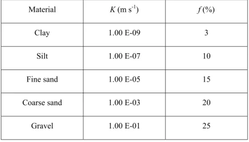
The soil hydraulic properties, K (m s-1) and f (-), for the numerical experiments were taken from Smith and Wheatcraft (1992) (see Table 1). During the simulations each pair of hydraulic properties was kept constant and uniform over the entire flow domain.
Numerical model sensitivity analysis X- and Z-discretization
For cases published in literature on the comparison between analytical solutions and the output of numerical models, usual aquifer configurations are: B=200 m and D=2 m (Brutsaert, 1994); B=400 m and D=10 m (Szilagyi et al., 1998);
B=100 m and D=1.5 m (Verhoest and Troch, 2000; Verhoest et al., 2002;
Pauwels et al., 2003; Huyck et al., 2005); B=100 m and D=2 m (Troch et al., 2002, 2003 and 2004). For the assessment of the sensitivity of the model output to the spatial discretization a reference geometry of B=100 m and D=2 m was selected. Maintaining this geometry, various simulations were carried out progressively reducing the column width along the aquifer domain (x direction) from 2 to 0.25 m. Each simulation run was repeated for the 5 material classes of which the hydraulic properties are listed in Table 1. A similar analysis was performed for the number of layers, varying from 1 to 8 layers with equal thickness.
Recession curves of 300 days were computed for the different grid systems using one-day time step and compared to the analytical solution of Boussinesq (Eq.
(10)). The outlet by a fully penetrating stream was mimicked by a cell with a prescribed head of 0.005 m, small enough to be consistent with Boussinesq’s (1903) assumption. The initial condition, a realistic piezometric profile, was obtained with a steady-state simulation considering a constant recharge rate, all along the upper boundary of the flow domain. The recession curves were then computed with a transient-state simulation starting from the above described initial condition with a zero recharge rate. For each mesh, the simulated discharge is normalized with respect to the Boussinesq analytical solution, from which the apparent bias R=Qsim/QBouss and deviations (Eq. (15)) are calculated and expressed in percent: Bouss Bouss sim Q Q Q Deviation (%)=100* − (15)
The bias and deviation between the simulated and the Boussinesq flowrates reveal that the simulation results for clay and silt are sensitive to the column width variation. However, results for fine sand, coarse sand and gravel are considerably less affected. When the number of layers with equal thickness increased, clay results showed that one layer configuration had the least mean apparent bias and mean deviation, when the aquifer in the z direction was split in four equal horizontal layers. For silt and fine sand, increasing from one to four layers had slight effects only, and the results for coarse sand were opposite to those for clay. The lowest variations were found for the four layers configuration, and the largest for the one layer condition. The mean apparent bias and mean deviation did not differ much for a one to four layer configuration in gravel. The conclusion with respect to the number of horizontal layers in which the aquifer is discretized, based on the match between the simulated output and the output of the
corresponding analytical solution, is that a one layer geometry is most recommendable when the domain is composed of fine materials such as clay and silt, while four or more layers should be considered for coarse sand and gravel aquifers.
Time discretization
The sensitivity of the output of the numerical model was also determined with respect to the time step. Since in previous analysis the deviation between the simulated recession and the recession curves obtained with the Boussinesq equation were smallest for the coarse sand material, also for the time discretization analysis a coarse sandy aquifer was assumed. Four simulations with time step 0.5, 1, 5, and 10 days were performed for a recession period of 300 days (Fig. 5). The results in Fig. 5 show that except for the 10 day case (-7.9% mean deviation) there is not much difference between a time step of 0.5 and 5 days, having the smallest deviation, respectively 0.89% and 0.97%, for a 0.5 and 1 day time step. For practical reasons a 1 day time step was used in all the simulations.
Sensitivity to aquifer geometry and soil hydraulic properties
Since analytical approximations (Eqs. 4, 7, 8 and 10) are dependent on the aquifer geometry, a sensitivity analysis was performed to assess the effect of different aquifer configurations. As in previous sections, the hydraulic conductivity and drainable porosity for coarse sand were used. Progressively B values were modified from 50 to 450 m (with 50 m increments), keeping D=2 m constant. Subsequently, it was found that two combinations of aquifer geometry yielded the least differences in their recession curves with respect to the Boussinesq long-time quadratic solution, i.e. B=100 m with D=2 m, and B=200 m with D=4 m. This result suggests that a ratio D/B=1/50 might be the most adequate for having the
least differences in recession curves. In order to verify the validity of this ratio four different cases with the same ratio were analyzed: D=0.5 m with B=25 m,
D=4 m with B=200 m, D=8 m with B=400 m, and D=16 m with B=800 m. Simulations for each case, and different soil hydraulic properties, were performed. Deviations calculated with Eq. (15) are presented in Fig. 6.
For clay (Fig. 6a) the effect of the scale is practically zero, having for the considered geometric configurations mean deviation values of 16%. When silt is considered (Fig. 6b) mean deviations range from 15.8 to 11.7%, corresponding to
DxB=16x800 m and DxB=0.5x25 m, respectively. For fine sand (Fig. 6c) variations in the mean deviations range from 9.7 to 2.0% for DxB=16x800 m and
DxB=0.5x25 m. For coarse sand (Fig. 6d), except for the smallest domain configuration (DxB=0.5x25 m), with mean deviation of -19.5%, others have mean deviation values of around 1.0%. For gravel (Fig. 6e) a mean deviation value of -86.7% is found for the smallest domain (DxB=0.5x25 m) and a mean deviation of 2.7% for the largest domain (DxB=16x800 m). These results suggest that for fine materials (such as clay and silt) smaller domains lead to smaller differences between the results of the numerical model and the Boussinesq solution, while large domains are preferred for coarser aquifer materials. When the effect of the different aquifer materials was analyzed, it was found that the recession curves from the numerical model when compared to the Boussinesq long-time analytical solution, present larger variations primarily for the finer materials considered (clay, silt), having mean deviations of 16% to 12%. However, for fine sand, coarse sand and gravel these deviations are less than 10%, particularly coarse sand, with mean deviation values are around 1.0%.
Typical values of hydraulic conductivity and drainable porosity found in the literature, when analytical solutions to the non-linear Boussinesq equation are tested (synthetic cases) versus the output of numerical models are:
K=8E-4 (m s-1) and f=0.34 (Verhoest et al., 2000; Huyck et al., 2005); K=1E-3 (m s-1) and f=0.34 (Verhoest and Troch, 2002), K=3E-4 (m s-1) and f=0.3 (Troch et al., 2002, 2003 and 2004); K= 8E-4 (m s-1) and f=0.33 (Basha and Maalouf, 2005); or K= 6E-4 (m s-1) and f=0.1(Pulido-Velazquez et al., 2006). These values indicate that so far the match between numerical and analytical solutions has been examined for a limited range of aquifer materials, corresponding in most of the cases to fine sands according to the range of aquifer properties listed in Table 1. The range of variation in the deviations for the different aquifer materials analyzed (see Fig. 6) urge that when analytical solutions are compared with numerical models that the values of hydraulic properties are carefully taken into consideration. In the present research, results suggest that the Boussinesq long-time quadratic equation, when compared to numerical model output, is better suited for materials such as fine or coarse sands, while in materials such as gravel, larger differences can be expected. Effects of the different materials are further described in results and discussion section.
Applied geometry and discretization scheme
As a result of the sensitivity analyses the adopted geometry and discretization for the comparative analysis of the three cases described in flow domain section for horizontal conditions are: length of the flow domain (taken orthogonal to the draining stream) B=400 m, aquifer thickness D=8 m; length parallel to the stream
When a sloping aquifer is considered, there are two options to present geometry in a numerical model. The first would be to simulate exactly the same inclined aquifer geometry, which is not possible in MODFLOW. The second option, is setting the flow domain to Bx=Bcos(i) and Dz=D/cos(i) in order to preserve the cross-sectional area (Fig. 3). This latter option has been adopted and the differences in the simulation results, consequence of the different flow domains, have proven to be insignificant partly because of the very small difference in width and depth found with the new settings.
Initial conditions
The first initial condition was obtained with the numerical model (with the chosen geometry and discretization as defined in the previous section) simulating the drainage of a fully saturated aquifer domain, and considering the groundwater profile when the head becomes smaller than D for x=B (see Fig. 8) as initial condition. Another way of obtaining the initial condition is assuming a constant recharge along the upper boundary of the numerical model, generating a realistic steady-state piezometric profile with a hydraulic head reaching D for x=B. In Fig. 8 these two initial conditions are compared to the inverse incomplete beta function
φ(2/3, 1/2), as proposed by Boussinesq (1904) (see Polubarinova-Kochina, 1962; Rupp and Selker, 2005). Figure 8 reveals that the profile obtained assuming a constant recharge matches closely the initial condition proposed by Boussinesq. Figure 8 also shows that the initial condition obtained through the drainage of a fully saturated domain differs significantly from the two other initial conditions, i.e. the water profile obtained under constant recharge and the inverse beta function. The difference may suggest that using the short-time equation (Eq. (13)), which is said to be valid before the wave reaches the end of the aquifer
(x=B), and subsequently the long-time Boussinesq equation (as suggested in Troch et al., 1993) may not be adequate. Model results show that the water table profile, starting with a fully saturated condition (the same as the short-time equation; see Eq. (13)), when reaching the end of the aquifer, x=B, is different to the one suggested by Boussinesq (inverse incomplete beta function initial condition profile); consequently leading to different recession curves.
Since in the present work the comparative analysis will be carried out only starting when the wave reaches x=B, when the Boussinesq long-time solution is said to be valid, no further discussion is presented for the fully saturated initial condition and the sensitivity analyses presented here after are carried out only with the infiltration by recharge and incomplete inverse beta function as initial condition.
Sensitivity to the initial conditions
As stated previously, the initial condition obtained assuming a constant recharge is quite similar to the one used by Boussinesq. In order to asses the effect of each initial condition, a sensitivity analysis was carried out following the methodology applied for the assessment of the X- and Z-discretization previously presented. The sensitivity analysis to the initial conditions was performed considering the hydraulic properties of the aquifer materials listed in Table 1. Results show that for the different materials studied, recession curves from the numerical model, using infiltration by recharge as initial condition, deviate generally least from the results obtained with Boussinesq long-time quadratic equation. Mean apparent bias and mean deviations using infiltration by recharge as initial condition, are in general less when compared to equivalent values using the inverse incomplete beta function profile. From this it can be concluded that even though the
differences in the two initial conditions seem to be small, when fine materials are considered (particularly clay), results are quite sensitive to the considered initial condition. In coarse materials, such as gravel, the two tested initial conditions have practically no influence on the recession curve. Since infiltration by recharge as initial condition showed the least influence on the mean deviation between the output of the numerical model and the analytical solution, this initial condition was selected for the comparative analysis, which is presented in the following section.
Results and discussion
The results of the comparative analysis of the recession outflows derived with the analytical solutions and the numerical model are presented in here. Differences between the methods are expressed in percent deviation (Eq. (15)). The geometry, the discretizations and the initial and boundary conditions used in MODFLOW were defined in the numerical model sensitivity analysis section. The results are presented according to each flow domain case.
Case 1: Horizontal aquifer floor
Two analytical approximations for an aquifer with an horizontal floor, i=0, were used for comparison of the recession outflow with the outflow generated using MODFLOW. The first one is given in Eq. (8) (Brutsaert, 1994), which is referred from now on as the exponential solution, and the second one is the so-called “exact” Boussinesq quadratic long-time analytical solution (Eq. (10)). The percent deviations for the five materials (see Table 1) are shown in Fig. 9 for a recession period of 300 days. Figures 9a and 9b illustrate that for clay and silt the outflow of the numerical model matches exactly the outflow calculated with Brutsaert’s exponential equation. The mean percent deviation between both
outputs is within -0.1 and 0.1%. The best match was obtained by putting p=0.5. The outflows generated by Boussinesq’s quadratic solution deviate on average with 15% (silt) to 16% (clay) from the MODFLOW outflows, and this throughout the entire recession period. The observed difference is somehow unexpected since MODFLOW solves Eq. (14) assuming that the flow is essentially (or practically) horizontal (i.e., the Dupuit assumption). It is believed that the observed difference is due to the initial condition which in the quadratic long-time analytical solution and MODFLOW is different.
The deviations for fine sand, coarse sand and gravel are depicted in the Figs. 9c, 9d and 9e, respectively. In contrast to the fairly constant percent deviation during the entire recession period observed for clay and silt, for the coarser materials the calculated deviations vary with time. For fine sand the outflow generated with Brutsaert’s exponential equation deviates from 13% (t=0) to -7% (t=300 days), with mean deviation of 0.3%; the approach is not valid for coarse sand since deviations in the first 127 days varied from -34% up to 800%; similarly the exponential equation does not hold for gravel. For fine sand the p factor was calibrated at 0.44. The deviations between the outflows generated with the Boussinesq quadratic equation and the model for fine sand, coarse sand and gravel show a rather similar pattern throughout the recession period, i.e. the percent deviation decreases with the recession time. For fine sand the percent deviation decreases from 16% (t=0) to 4% (t=300 days), with mean deviation 7%; the percent deviation varies only slightly with the recession time in the coarse sand aquifer, being on average 0.7%; and in gravel it drops from 23% at t=10 days to -5% for t=300 days, with mean deviation of 3%.
The comparative analysis reveals that Brutsaert’s exponential analytical solution is mainly valid for fine materials. This can be partly explained by the fact that the numerical model recession curves present a linear behaviour for those materials. For coarser materials, such as fine and coarse sand, this is not the case and numerical model results show a non-linear behaviour, being most clear for the gravel aquifer (Fig. 9e). From this, it is concluded that the exponential approach is less capable of reproducing the outflow of coarse aquifers with a horizontal floor, and that the percent deviation increases the coarser the material of the aquifer. In general, notwithstanding the percent mean deviations found for clay and silt, between 16 and 15% respectively, which seems to be the consequence of the assumed initial condition, the numerical generated outflows seems to agree mostly with the outflows obtained using the Boussinesq quadratic analytical equation, indicating that the quadratic approach best mimics the non-linear behaviour of the groundwater flow.
Case 2: Sloping aquifer floor
The percent deviation between the outflows generated with MODFLOW and Brutsaert’s (1994) analytical solution for aquifers with a sloping floor of 0.5, 1, 2, 5 and 10% composed of clay, silt, fine sand, coarse sand and gravel are presented in Fig. 10a, b, c, d and e. Here again the trend in percent deviation for clay and silt are quite similar, as it was the case for the horizontal aquifer floor. For slope angles of 0.5% and 1% the mean percent deviations are within the order of 0.3% to 0.7%, whereas within the first 30 (clay) to 10 days (silt) the percent deviation drops from respectively 40 and 30% to nearly 0%. For sloping aquifer floors of 2, 5 and 10% mean percent deviations found for clay were 68, 80 and 93%, and -74, -80 and -93% for silt. The percent deviation between the modelled outflow
recession time behaves very similar than for clay and silt. Aquifer slopes 0.5% and 1%, having mean percent deviations of 0.14% and 3%, showed a tendency of increasing percent deviation as from t=100 days onwards, reaching for the 1% slope case a percent deviation of 8% at t=300 days. For coarser aquifer material, such as coarse sand and gravel, the numerical model is not able of generating similar outflows in comparison to the outflows obtained with Eq. (7). The percent deviations vary strongly from negative to very large positive values within a short period as depicted in Fig. 10d (coarse sand), and deviations can even not be assessed with the numerical model for gravel aquifers (Fig. 10e): the main reason is that the aquifer dries out. As can be seen in Figs. 10d and 10e the time that the aquifer becomes dry decreases as the slope of the aquifer floor increases and the aquifer material is coarser.
The analysis revealed that the value of the p factor had little effect for slopes above 1%, whereas the optimal value for the slope of 0.5 and 1% by calibration was found to be within 0.5<p<0.7. From the Figs. 10a (clay), b (silt) and c (fine sand) it can be seen that for slopes larger than 1% the percent deviations increase rapidly. This can be explained reformulating the dimensionless parameter -aB in Eq. (7) as: pD B i aB=tan( ) /2 − (16)
This parameter represents the relative magnitude of the slope term, i.e., the gravity versus the diffusion term. Its value increases with slope i, and with the shallowness (B/D) of the aquifer. When small i values are considered, according to Brutsaert (1994), the flow problem can be treated as a horizontal flow case, and Eq. (8) can be used. However, Brutsaert (1994) quotes that slopes of 0.01% may
not be all that small and their effects should be considered. At the contrary the results presented in Fig. 10 suggest that cases with slopes up to 1% may be treated as horizontal flow cases. When large values of -aB are present, diffusion becomes small and q decays mostly because gravity flow, due to the steepness of the slope, overtakes diffusive flow. According to Brutsaert (1994) the solution presented in Eq. (7) is likely to become less reliable in describing accurately the free surface outflow because of the inherent limitations in the hydraulic approach. Furthermore, the effect of the dimensionless parameter, unlikely resembles the real effect of gravity found in hillslopes. (-aB) increases proportionally as the aquifer floor slope i increases. When it is expressed as e-aB, as in Eq. (16), the effect of this term is determinant. In Fig. 11 log(e-aB) is plotted as a function of
the aquifer floor slope illustrating that the effect of slope gradually becomes more important as the slope increases. The difference in log(e-aB) for aquifer slopes of
0.5 and 1% is relative small (the same order of magnitude) compared to the difference found for slopes above 1% (several orders of magnitude). In conclusion, the results presented in Fig. 10 suggest that the effect of gravity might be overestimated in Brutsaert’s exponential expression (Eq. (16)) when compared to the results obtained with the numerical model.
Case 3: Concave aquifer floor
The outflow generated with the numerical model for a concave aquifer floor, with
H equal to 0.4, 0.8, 1.6, 3.2 and 6.4 m, was compared to the outflow using
Boussinesq’s equation (Eq. (4)). As could be expected the trends in percent deviations found for the cases (clay, silt, fine sand, coarse sand and gravel) with concave floor (Fig. 12) are very similar to the trends presented for those of the same material with horizontal floor (Fig. 9). This should not surprise since, as
Brutsaert’s exponential equation used for the horizontal floor case. The C factor in Eq. (4), which Boussinesq defined as being dependent on the initial condition, was defined by trial and error similarly to the way the p factor was derived. Figure 12a illustrates that for all H values the numerical model yields nearly the same outflows as the analytical approach and this for the entire recession period of 300 days, with mean percent deviation of 0.4%. A similar conclusion can be drawn for silt, showing a mean percent deviation of -2%. For a fine sand aquifer the percent deviation between the outflow generated with the analytical solution and MODFLOW tends to be larger than for clay and silt, ranging from 9% for t=0 to nearly -9% for t=300 days, having a mean percent deviation of -1%. Figure 12c also shows that the percent deviation in outflow between both approaches decreases as the value of H increases. For aquifers composed of coarse sand and gravel the exponential equation does not yield the same outflows as the outflows simulated with MODFLOW. For coarse sandy aquifers the percent deviations for all H values was of the order of 2% for t=0, decreasing to nearly -20% and increasing to unacceptable values after 20 to 50 days. For gravels, just as for aquifers with horizontal floor, the percent deviation between the analytical generated outflows and the simulated outflows were already out of range after 1 to 2 days of recession. It is observed that the percent deviation between the outflows generated with the analytical approximation and MODFLOW, tends to be larger for increasing H values and particularly when coarse materials are considered (see Fig. 12). These results may also suggest that under such conditions, the assumption that the streamlines are approximately parallel to the aquifer floor (see Boussinesq, 1877), may no longer be acceptable.
Conclusions
During the last century, analytical solutions have been extensively used to predict the outflow of homogeneous unconfined hillslope aquifers. Although recently new aspects were integrated as to make the analytical solutions applicable for more conditions, analytical solutions in general are based on strong simplification of the reality and therefore only valid for well defined conditions. In the present research a comparative analysis was conducted between different analytical approximations of the non-linear Boussinesq equation and the numerical solution of the receding flow of an unconfined homogeneous aquifer in MODFLOW, whereby the simulated outflows were considered the reference. The percent deviation in outflow, calculated with an analytical approximation and numerical model, for a homogeneous aquifer with varying geometry and hydraulic properties was used as evaluation criteria. Prior to the comparative analysis a sensitivity analysis was carried out as to identify for the numerical model the aquifer geometry, scale and the space and time discretization to get the best match between the analytical and numerical generated recession curves. An aquifer geometry with D/B ratio of 1/50, D=8 m and B=400 m, ∆x=2 m, ∆z=2 m, and time step of 1 day was found to provide the best match.
For aquifers with a horizontal floor it has been shown that Brutsaert’s exponential solution is primarily valid for clay and silt materials, but fails to reproduce the receding outflow for fine and coarse sand and gravel aquifers. The deviation to the reference receding outflows simulated with the numerical model increases the coarser the aquifer material, being most striking for the gravel aquifer. Boussinesq’s quadratic analytical solution better reproduces the receding outflows of fine and coarse sand and gravel aquifers. Results presented herein suggest that
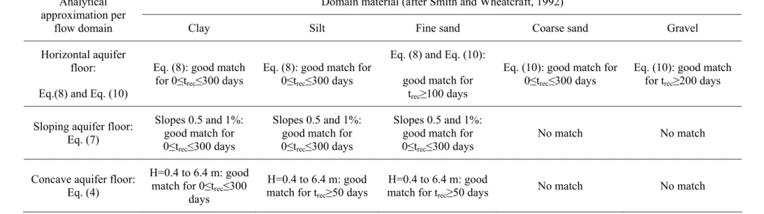
the issue of linearity and non-linearity, stressed by different authors (Hall, 1968; Burtsaert and Lopez, 1998; Wittenberg, 1999; Dewandel et al., 2003; among others) is strongly related to the properties of the aquifer medium. For hillslope aquifers with a uniform sloping floor it has been demonstrated that, for slopes larger than 1%, the outflows obtained with Brutsaert’s analytical solution increasingly deviate from the MODFLOW simulated outflows, and that the percent deviation increases the coarser the aquifer medium. Brutsaert’s analytical solution does not yield acceptable values for coarse sand and gravel aquifers, most likely because the effect of gravity might be overestimated with this particular expression. The analytical solution for aquifers with concave floor, having an exponential form, produces up to a certain extent similar outflows as MODFLOW. However, as the case of the horizontal aquifer floor, the exponential equation is proven to be primarily valid for fine medium aquifers. Table 2 gives a summary of the researched conditions for which the analytical approximations yield a similar output as the numerical solution of the general groundwater flow equation, using MODFLOW as code.
Summarizing, this comparison of recession outflow for a hillslope aquifer calculated by analytical solutions and numerical models (in this case MODFLOW), for checking the agreement between the analytical and numerical solution are only valid for certain ranges of hydraulic properties of the aquifer medium, the geometry of the flow domain and the initial and boundary conditions. It is here underlined, that the results presented were obtained for homogeneous aquifers, and it is to be expected that the ranges for which the analytical approximations yield similar results to those of the numerical model, will be different for heterogeneous aquifers.
Acknowledgments The first author acknowledges financial support from the Katholieke Universiteit Leuven (K.U.Leuven), under the Selective Bilateral Agreements with Latin American Universities. The authors are grateful to the reviewers and editors.
References
Basha HA, Maalouf SF (2005) Theoretical and conceptual models of subsurface hillslope flows. Water Resour Res 41 W07018 doi:10.1029/2004WR003769.
Beven K (1981) Kinematic subsurface storm flow. Water Resour Res 17: 1419-1424.
Boussinesq J (1877) Essai sur la théorie des eaux courantes du mouvement nonpermanent des eaux souterraines. Acad Sci Inst Fr 23: 252-260.
Boussinesq J (1904) Recherches théoriques sur l’écoulement des nappes d’eau infiltrées dans le sol et sur le débit des sources. J Math Pure Appl 10: 5-78.
Brutsaert W, Nieber JL (1977) Regionalized drought flow hydrographs from a mature glaciated plateau. Water Resour Res 34: 233-240.
Brutsaert W (1994) The unit response of groundwater outflow from a hillslope. Water Resour Res 30: 2759-2763.
Brutsaert W, Lopez JP (1998) Basin-scale geohydrologic drought flow features of riparian aquifers in the southern Great Plains. Water Resour Res 34(2): 233-240.
Charbeneau RJ (2000) Groundwater Hydraulics and Pollutant Transport. Prentice Hall, Upper Saddle River, NJ: 48-49.
Dewandel B, Lachassagne P, Bakalowicz M, Weng Ph, Al-Malki A (2003) Evaluation of aquifer thickness by analysing recession hydrographs. Application to the Oman ophiolite hard-rock aquifer. J Hydrol 274: 248-269.
Hall FR (1968) Base-flow recession-A review. Water Resour Res 4: 973-983.
Henderson FM, Wooding RA (1964) Overland flow and groundwater flow from a steady rainfall of finite duration. WJ Geophys Res 69: 1531-1540.
Horton RE (1933) The role of infiltration in hydrologic cycle. Trans Am Geophys Union 14: 446-460.
Huyck AAO, Pauwels VRN, Verhoest NEC (2005) A base flow separation algorithm based on the linearized Boussinesq equation for complex hillslopes. Water Resour Res 41 W08415 doi: 10.1029/2004WR003789.
Kraijenhoff van de Leur DA (1979) Rainfall-runoff relations and computational methods. Publication 16: 245-320. ILRI Wageningen Netherlands.
Long AJ, Derickson RG (1999) Linear system analysis in a karst aquifer. J Hydrol 219: 206-217. McDonald MG, Harbaugh AW (1988) A modular three-dimensional finite-difference
ground-water flow model. Techniques of Water-Resources Investigations US Geol Surv Book 6 Ch A1.
Maillet E (1905) Essais d’hydraulique souterraine et fluviale. Librairie Sci A Hermann Paris 218. Mendoza GF, Steenhuis TS, Walter MT, Parlange J-Y (2003) Estimating basin-wide hydraulic
parameters of a semi-arid mountainous watershed by recession-flow analysis. J Hydrol 279: 57-69.
Nathan RJ, McMahon TA (1990) Evaluation of automated techniques for baseflow and recession analysis. Water Resour Res 26: 1465-1473.
Paniconi C, Troch P, van Loon EE, Hilberts AG (2003) Hillslope-storage Boussinesq model for subsurface flow and variable source areas along complex hillslopes: 2. Intercomparison with a three-dimensional Richards equation model. Water Resour Res 39(11): 1317
doi:10.1029/2002WR001730.
Parlange JY, Stagnitti F, Heilig A, Szilagyi J, Parlange MB, Steenhuis TS, Hogarth WL, Barry DA, Li L (2001) Sudden drawdown and drainage of a horizontal aquifer. Water Resour Res 37(8): 2097-2101.
Pauwels VRN, Verhoest NEC, De Troch FP (2003) Water table profiles and discharges for an inclined ditch-drained aquifer under temporally variable recharge. J Irrig Drain Eng 129(2): 93-99.
Polubarinova-Kochina PY (1962) Theory of Groundwater Movement. Princeton University Press New Jersey p.613.
Pulido-Velazquez DA, Sahuquillo DA, Andreu J (2006) A two-step explicit solution of the Bousinesq equation for efficient simulation of unconfined aquifers in conjuctive-use models. Water Resour Res 42 W05423 doi:10.1029/2005WR004473.
Rupp DE, Selker JS (2005) Drainage of a horizontal Boussinesq aquifer with a power law hydraulic conductivity profile. Water Resour Res 41 W11422 doi:10.1029/2005WR004241. Shevenell L (1996) Analysis of well hydrographs in a karst aquifer: estimates of specific yields
and continuum transmissivities. J Hydrol 174: 331-355.
Serrano SE, Workman SR (1998) Modeling transient stream/aquifer interaction with the non-linear Boussinesq equation and its analytical solution. J Hydrol 206: 245-255.
Smith L, Wheatcraft SW (1992) Groundwater flow. In: Handbook of Hydrology (D.R. Maidment, Ed.), 6.1.-6.58.
Szilagyi J Parlange MB, Albertson JD (1998) Recession flow analysis for aquifer parameter determination. Water Resour Res 37: 1851-1857.
Troch P, De Troch F, Brusaert W (1993) Effective water table depth to describe initial conditions prior to storm rainfall in humid regions. Water Resour Res 29: 427-434.
Troch P, van Loon EE, Hilberts A (2002) Analytical solutions to a hillslope-storage kinematic wave equation for subsurface flow. Adv Water Resour 25: 637- 649.
Troch P, Paniconi C, van Loon EE (2003) The hillslope-storage Boussinesq model for subsurface flow and variable source areas along complex hillslopes: 1. Formulation and characteristic response. Water Resour Res 39(11): 1316 doi:10.1029/2002WR001728.
Troch P, van Loon AH, Hilberts A (2004) Analytical solution of the linearized hillslope-storage Boussinesq equation for exponential hillslope width functions. Water Resour Res 40(8): W08601 doi: 10.1029/2003WR002850.
Verhoest NEC, Troch P (2000) Some analytical solutions of the linearized Boussinesq equation with recharge for a sloping aquifer. Water Resour Res 36(3): 793-800.
Verhoest NEC, Pauwels VRN, Troch P, De Troch FP (2002) Analytical solution for transient water table heights and outflows from inclined ditch-drained terrains. J Irrig Drain Eng 128(6): 358-364.
Vogel RM, Kroll CN (1992) Regional geohydrologic-geomorphic relationships for the estimation of low-flow statistics. Water Resour Res 28: 2451-2458.
Wittenberg H (1999) Baseflow recession and recharge as nonlinear storage processes. Hydrol Process 13: 715-726.
Figure 1: Conceptual drawing of the cross-section of a hillslope aquifer with inclined slope
Figure 2: Sketch of Boussinesq (1877) conceptual model
Figure 3: Schematic presentation of an aquifer with sloping floor as used in the numerical model
Figure 4: Sketch of Boussinesq (1877) conceptual model for a concave aquifer floor
Figure 5: Variation of the percent deviation between the simulated outflows and the outflow generated with the Boussinesq equation for a coarse sand aquifer as a function of the time step [(x) = 0.5 days; ({) = 1 day; () = 5 days; (▲) = 10 days]
Figure 6: Results of the sensitivity analyses with respect to the size of the domain [triangles (▲): D = 16 m and B = 800 m; squares (): D = 8 m and B = 400 m; circles ({): D = 4 m and B = 200 m; crosses (x) D = 0.5 m and B = 25 m] and aquifer materials [(a) clay; (b) silt; (c) fine sand; (d) coarse sand; and (e) gravel] Figure 7: Schematic presentation of the geometry of the numerical model of a homogeneous aquifer with horizontal floor; discretization of 2 m in the x- and z-direction (not to scale); black square () depicts the outlet with imposed potential Figure 8: Graphical presentation of the three different initial conditions at the top of the aquifer. Dashed dotted line: water table profile obtained by drainage of a fully saturated aquifer; dashed line: water table profile obtained under constant recharge; and solid line: the inverse incomplete beta function (Boussinesq, 1904; Polubarinova-Kochina, 1962; Rupp and Selker, 2005)
Figure 9: Deviation between the simulated flow and the flow derived using Boussinesq’s quadratic (x) and Brutsaert’s exponential ({) solution, for a homogeneous aquifer with horizontal floor and different K and f values [(a) clay; (b) silt; (c) fine sand; (d) coarse sand; and (e) gravel]
Figure 10: Deviation between the simulated flow and the flow derived using Brutsaert’s sloping aquifer floor solution for different slopes (x 0.5% slope; { 1%
slope; ▲ 2% slope and 5% slope) and aquifer materials [(a) clay; (b) silt; (c) fine sand; (d) coarse sand; and (e) gravel]
Figure 11: Logarithm of the exponential form of the dimensionless parameter –
aB (Eq. (16)) as a function of slope of the aquifer floor
Figure 12: Deviation between the simulated flow and the flow derived using Boussinesq’s concave aquifer floor solution for different concave depths [(x) H = 0.4 m; ({) H = 0.8 m; (▲) H = 1.6 m; () H = 3.2 m; and (□) H = 6.4 m] and aquifer materials [(a) clay; (b) silt; (c) fine sand; (d) coarse sand; and (e) gravel]
Table 1: Representative values for K and f (after Smith and Wheatcraft, 1992)
Material K (m s-1) f (%)
Clay 1.00 E-09 3
Silt 1.00 E-07 10
Fine sand 1.00 E-05 15
Coarse sand 1.00 E-03 20
Table 2: Ranges for which the analytical approximations match the recession outflows of a homogeneous hillslope aquifer generated with MODFLOW
Domain material (after Smith and Wheatcraft, 1992) Analytical
approximation per
flow domain Clay Silt Fine sand Coarse sand Gravel
Horizontal aquifer floor: Eq.(8) and Eq. (10)
Eq. (8): good match for 0≤trec≤300 days
Eq. (8): good match for 0≤trec≤300 days
Eq. (8) and Eq. (10): good match for
trec≥100 days
Eq. (10): good match for 0≤trec≤300 days
Eq. (10): good match for trec≥200 days
Sloping aquifer floor: Eq. (7)
Slopes 0.5 and 1%: good match for 0≤trec≤300 days
Slopes 0.5 and 1%: good match for 0≤trec≤300 days
Slopes 0.5 and 1%: good match for 0≤trec≤300 days
No match No match
Concave aquifer floor: Eq. (4)
H=0.4 to 6.4 m: good match for 0≤trec≤300
days
H=0.4 to 6.4 m: good match for trec≥50 days
H=0.4 to 6.4 m: good
match for trec≥50 days No match No match
Fig.1
Fig.3