HAL Id: hal-00346013
https://hal.archives-ouvertes.fr/hal-00346013
Submitted on 10 Dec 2008
HAL is a multi-disciplinary open access archive for the deposit and dissemination of sci-entific research documents, whether they are pub-lished or not. The documents may come from teaching and research institutions in France or abroad, or from public or private research centers.
L’archive ouverte pluridisciplinaire HAL, est destinée au dépôt et à la diffusion de documents scientifiques de niveau recherche, publiés ou non, émanant des établissements d’enseignement et de recherche français ou étrangers, des laboratoires publics ou privés.
LCD motion blur estimation using different
measurement methods
Sylvain Tourancheau, Kjell Brunnström, Borje Andrén, Patrick Le Callet
To cite this version:
Sylvain Tourancheau, Kjell Brunnström, Borje Andrén, Patrick Le Callet. LCD motion blur estimation using different measurement methods. Journal of the Society for Information Display, Society for Information Display(AIP), 2009, 17 (3), pp.239-249. �10.1889/JSID17.3.239�. �hal-00346013�
LCD motion blur estimation using different measurement methods
Sylvain Tourancheau ¹, Kjell Brunnström ², Borje Andrén ² and Patrick Le Callet ¹ ¹ IRCCyN, IVC Group - University of Nantes
Polytech’Nantes – Site de la Chantrerie rue Christian Pauc
44306 Nantes – France
[email protected] [email protected]
² Netlab: IPTV, Video and Display Quality - Acreo AB Electrum 236
SE-164 40 Kista – Sweden [email protected]
Abstract: The primary goal of this study is to find a measurement method for motion blur which is easy to carry out and gives results that can be reproduced from one lab to another. This method should be able to also take into account methods for reduction of motion blur such as backlight flashing. Two methods have been compared. The first method uses a high speed camera that permits us to directly picture the blurred edge profile. The second one exploits the mathematical analysis of the motion blur formation to construct the blurred edge profile from the temporal step-response. Measurement results and method proposals are given and discussed.
1 Introduction
The picture quality of liquid crystal displays (LCD) has come a long way, through massive research and development, and have in many aspects surpassed display based on cathode ray tubes (CRT) in performance e.g. luminance, contrast and color gamut. However, LCDs have still not been able to match CRTs when it comes to motion rendering. Despite recent improvements to LCD technology such as response time compensation (i.e. overdrive), LCD motion blur remains very annoying for sequences with rapid movements. In fact, even if the response time of a liquid crystal matrix was reduced to zero, motion blur would still be visible. This is due to sample-and-hold behavior of the display; the light intensity is sustained on the screen for the duration of the frame, whereas on a CRT light intensity is a pulse which fades over the frame duration [10] (cf. Figure 1). The main difference happens when the eyes of the observer are tracking a moving object on the screen; for a given frame, the picture is sustained on the screen while the eyes are still moving slightly anticipating the movement of the object. Edges of this object are integrated on the retina while moving, resulting in a blur [5].
The most common metric to characterize LCD motion blur is the motion picture response time (MPRT) [7] [11] and its relative indexes blurred edge time ( BET ) and blurred edge width ( BEW ). A lot of measurement systems have been developed in order to measure MPRT [1], but they are generally quite expensive and the measurements are fairly complicated to carry out. As a consequence, alternative approaches have been proposed, based on the theoretical analysis of the spatial and temporal apertures of the display. It has been shown that MPRT can be obtained from the temporal impulse response [4] [8] or from the temporal step response [6] [15] instead of measuring the blur width spatially. Earlier comparisons between the results of methods using
temporal response measurements and those using camera measurement systems have shown that both approaches are very close [1] [3].
TCO Requirements provide well known and recognized quality labels for displays. For these requirements to remain useful, they must continuously be reviewed and updated when necessary. Today there is a requirement concerning the response time in TCO’06 Displays [13], but none concerning LCD motion blur. Besides, the requirements concerning response time are not sufficient to guarantee a low level of motion blur. The primary goal of this study is to find a measurement method of motion blur which is easy to carry out and which can be reproduced from one lab to another with a limited variability.
Improvements are included in recent monitors in order to enhance their motion rendering performance. As a result, temporal responses strongly vary from one display to another, depending on what technologies that are used. Response time compensation can lead to overshoots and undershoots, pulse-width modulation (PWM) for backlight dimming introduces artifacts, and motion-blur reduction methods such as backlight-flashing (BF) modify the response shape to obtain a more impulse-type behavior. To determine response time values, the underlying step responses need to be filtered out but this process can affect the final value, as noted by TCO in their response time measurements. However, when performing motion blur characterization, these temporal variations must be kept and taken into account since they will modify, and hopefully reduce, the quantity of blur. We must be sure, though, that they will not affect the motion blur estimation.
For these reasons, further measurements must be done, on various displays, in order to analyze and compare the efficiency and reliability of the two described methods in the presence of motion blur reduction methods as mentioned above. In this paper, both measurement methods have been
carried out and applied on four displays with various temporal responses. Results from both spatial and temporal measurements are compared and discussed.
Figure 1: Temporal evolution of a pixel’s intensity for a CRT display (left) and for a LCD (right).
2 Definitions
In the following, we will consider a pixel changing its intensity from a start gray level N to a s
final gray level N . The considered gray-to-gray transition is written f Ns →Nf. The temporal response of the pixel is written ( )
s f
N→N t
R and RNs→Nf( )t is the normalized
1 temporal profile
between 0 and 1. The response time τ is defined as follows, according to recommendations [14]:
10%
90% 10% 10% 90%
90%
( ) 0.1
with and such as
( ) 0.9 s f s f s f N N N N N N t t t t t t τ → → → = = − = R R (1.1)
Now, we consider an edge moving from left to right, so each pixel of the screen will initially have the gray level of the right part of the edge Nright and then have the gray level of the left part
of the edge Nleft. As a consequence, the considered gray-to-gray transition is Nright →Nleft. The
1 ( ) ( ) (0) ( ) (0) t t = − ∞ − R R R R R
spatial profile of the moving edge is written ( )
right left
N →N x
E . Here again, ENright→Nleft( )x is the normalized spatial profile. The blurred edge width BEW is defined as follows:
10%
90% 10% 10% 90%
90%
( ) 0.1
with and such as
( ) 0.9 right left right left right left N N N N N N x BEW x x x x x → → → = = − = E E (1.2)
When there are several candidates for t10% and t90% (resp. x10% and x90%), they are chosen in
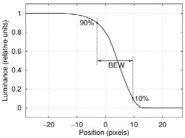
order to maximize τ (resp. BEW ). An example of blurred edge profile is given in Figure 2.
Figure 2: Example of blurred edge profile ENi→Nj( )x . BEW is measured between 10% and 90% of the edge dynamic.
3 LCD motion blur analysis
LCD motion blur analysis has been considered by several authors, notably by Pan et al. [8] and by Watson [15]. The treatment here follows these authors closely and is given here to make the article self-contained. From input signal to sensor, the formation of LCD motion blur on a moving object can be described in three steps as illustrated in Figure 3. First, the moving object is displayed by the LCD. Then, the sensor is tracking the moving object in order to stabilize it (it is
referred as smooth pursuit in the case of eyes). Finally, the stabilized object is integrated over time by the sensor.
Figure 3: Diagram of the motion blur formation.
3.1 Display rendering
We consider a sharp edge between two uniform areas with gray levels N (on the left-hand side) i
and N (on the right-hand side). This edge is moving from left to right with a constant speed v j
(in pixels per frame). In the spatial domain, variations only occur in one dimension, e.g. the motion direction. For simplification, we only consider one spatial dimension, horizontal one. At each new frame k , the pixels at positions x∈
[
kv…(k+1)v]
are subject to a temporaltransitionNi →Nj. As a consequence, the luminance signal emitted by the display D( , )x t , can
be expressed in the spatio-temporal domain by:
[
]
( , )x t = (t−kT) , ∀ ∈x kv...(k+1)v
D R (1.3)
This can be rewritten as:
( , )x t t floor x T , x v = − ∀ ∈ ℕ D R (1.4)
where T is the refresh period of the display and floor is the floor function that returns the largest integer less than its argument.
3.2 Sensor tracking
We consider that the sensor is perfectly tracking the edge moving at a constant velocity v (this is not exactly right when the sensor is the eye [11] but it can be assumed as a first approximation). As a consequence, the stabilized edge S( , )x t can be expressed in the spatio-temporal domain as:
( , ) ( , ) ( , ) . t x t x v t T x t x t t floor T v T = + = − + S D S R (1.5)
The stabilized edge pictured by the sensor is periodic with a one-frame period, at any position x .
3.3 Temporal integration
As a final step, the stabilized edge is integrated over time by the sensor. The spatial profile of the moving edge is then expressed by:
( ) ( , ) ( ) . j i j i j i N N N N N N x x t dt x t x t floor T dt v T +∞ → −∞ +∞ → −∞ → = = − +
∫
∫
E S E R (1.6)Because the signal S( , )x t is periodic with a one-frame period, the integral can be reduced over
any interval of this length. We choose the interval xT, T xT
v v
−
−
in order to simplify the floor function which is zero on this interval.
( )
( ) j i j i x T T V x N N N N T V x − t dt → =∫
− → E R (1.7)The integral can be then extended on an infinite interval by multiplying the temporal transition by a shifted one-frame wide rectangular function:
( )
( ) rect j i j i N N N N x x t t T dt v +∞ → −∞ → = ⋅ − ∫
E R (1.8)This relation corresponds to the following convolution:
( ) rect j i j i N N N N xT xT x v v → → − = ∗ E R (1.9)
The analysis shows that the spatial profile of a moving edge ( )
j i
N →N x
E tracked by a sensor can be obtained by a convolution of a temporal step-response ( )
j i
N →N t
R of a gray-to-gray transition with a unit window which has a width of one-frame-period.
4 Measurements 4.1 Displays under test
Four recent monitor displays have been tested in this work. They were all AM-TFT LCD with a refresh frequency of 60 Hz, with different types of panel, sizes and resolutions as depicted in Table 1. In the following, they are identified with letters from A to D2. Both C and D were using
backlight flashing (BF). The response time given by the manufacturers is also mentioned.
Id Type Size Resolution Lmax (cd/m²) RT (ms) Notes
A IPS 20’’ 1600x1200 300 8
B TN 24’’ 1920x1200 400 5
C IPS 26’’ 1920x1200 500 5 Backlight flashing D IPS 30’’ 2560x1600 370 5 Backlight flashing
Table 1: Specifications of displays under test. Lmax is the luminance of white, and RT the response time value given by the manufacturers.
2 Some preliminary results have been presented at the SID 2008 Symposium [S. Tourancheau et al., “Motion blur estimation on
LCDs,” SID Symposium Digest Tech. Papers 39, 1529-1532 (2008)]. This preliminary work concerned five displays but one of them has been removed in this extended version after we ascertained some irregularities in the measurement procedure of this display. As a consequence, display IDs has been modified between the two papers.
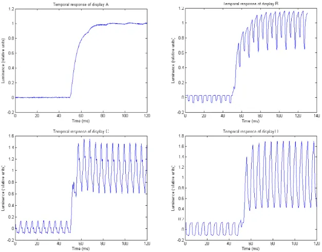
Figure 4: Temporal step-responses of the four displays under test, for the transition 0→255.
4.2 Temporal step-response measurements
For these measurements, the stimulus consisted of a sequence of gray patches ordered to measure 20 transitions from one gray level to another among five. Each gray patch was displayed during 20 frames. The following gray levels have been used: 0, 63, 127, 191, and 255.
The light intensity emitted by the display was read by a photo diode positioned in close contact with the screen surface. The photo diode was surrounded by black velvet in order to reduce any scratches to the display surface and to shield any ambient light reaching the photo diode. The
photo diode (Burr-Brown OPT101 monolithic photodiode with on chip transimpedance amplifier) has a fast response (28 µs from 10% to 90%, rise or fall time). The signal was read by an USB oscilloscope EasyScope II DS1M12 "Stingray" 2+1 Channel PC Digital Oscilloscope/Logger from USB instruments. The accuracy of the instrument has been tested with a LED light source connected to a function generator. The sampling time used for these measurements was 0.1 milliseconds. The sequence has been repeated at least 5 times and allows for averaging in order to avoid random noise.
Figure 4 illustrates the temporal step-responses of the four displays under test. We can notice backlight flashing on displays C and D, and pulse-width modulation on display B. In order to obtain the response time, these step-responses were filtered with a band-reject filter to take away overlaid frequencies induced by the pulse-width modulation or the backlight flashing. The response time values τ have been then calculated on the filtered signal according to recommendations [14] as described in Section 2.
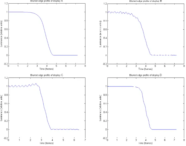
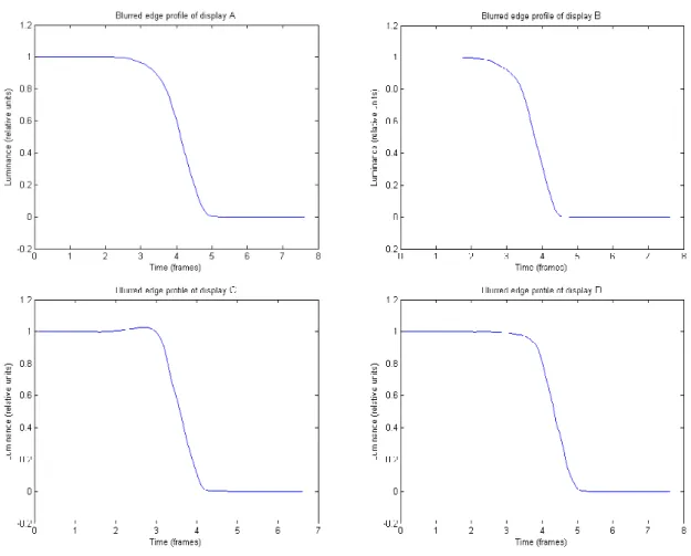
The blurred edge profiles were obtained using the analytic method described in Section 3 directly from the raw temporal data without any filtering because this would add blur components that are not actually present. The width of the blurred edge profile was then measured as illustrated in Figure 2. Here, we obtained directly the blurred edge time BET as the edge profile is measured on a time dimension. It will be denoted BET . Figure 5 illustrates the blurred edge profiles T
obtained from the temporal step-responses of the four displays under test.
It can be noticed that some residuals of the temporal artifacts are still visible, particularly for displays B and C. They are due to the fact that BF and PWM frequency is not a multiple of the display refresh frequency: the PWM frequency of display B is 204 Hz and the BF is 192 Hz. As a consequence, temporal modulations are not filtered out by the convolution with a window of
one-frame-period width. On the other hand, the BF frequency of display D is 180 Hz, which is a multiple of the display refresh frequency (60 Hz), and backlight modulations are perfectly removed by the convolution.
Figure 5: Blurred edge profiles of the four displays under test obtained from the temporal step-responses presented in Figure 4, for the transition 0→255.
4.3 Spatio-temporal measurements of a moving edge
The apparatus used for these measurements consisted of a high-frame-rate CCD camera and a PC used to control the camera, to store grabbed frames, and to display stimuli on the test display. A JAI PULNiX's Gigabit Ethernet CCD camera, the TM-6740GE, has been used for these measurements. It was linked to the control PC via Ethernet, using a Gigabit Ethernet Vision (GigE Vision) interface which permits to reach high frame-rate. Its frame-rate has been set to
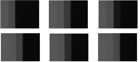
1200 Hz with a resolution of 224x160 pixels. The display frame-rate was set to 60 Hz, thus we obtain 20 CCD frames for each display frame. The distance between the measured display and the camera has been accurately adjusted in such a way that one pixel of the display array is pictured by 4x4 pixels on the CCD array. This permitted us to obtain a good approximation of the 56x40 pixels of the display by computing the mean of each 4x4 blocks in the CCD frame. Moreover, this quarter-pixel precision allowed us to perform accurate motion compensation and to reduce the acquisition noise that could have been added by the camera. One example of frames grabbed by the camera is shown in Figure 6.
Figure 6: Example of camera frames pictured during one display frame-period T on display A.
Figure 7: Blurred edge obtained after motion compensation and temporal summation of the camera frames, on display A for a transition 0→255.
Stimuli were generated with Matlab on a PC using the PsychToolbox extension [2]. They consisted of a straight edge moving from left to right. Three values could be set: the start gray level N which is the gray level of the right part of the screen, the final gray level s N which was f
the gray level of the left part of the screen, and the velocity v in pixels per frame. Five gray levels have been used in the measurements: 0, 63, 127, 191 and 255. Thus, 20 transitions have been studied. As mentioned before, the blurred edge profile was obtained by motion compensation of each CCD frames to simulate the tracking of the sensor. The high camera frame-rate and the precise calibration of the apparatus permitted us to achieve this motion compensation accurately. Next, all frames were added to each other to simulate the temporal integration of the sensor. An example of blurred edge obtained with this method is shown in Figure 7 for an edge moving with a velocity v = 10 pixels per frame. The blurred edge width BEW (in pixels) was computed as illustrated in Figure 2. The blurred edge time BET was computed by dividing
BEW by the velocity v :
/
BET =BEW v (1.10)
In the following, the blurred edge time obtained with this measurement method is written BET . S
Figure 8 illustrates the blurred edge profiles obtained from the spatial measurements for the four displays under test. These spatial profiles are plotted as a function of time by scaling the space domain with velocity v [15]. It can be noticed that the profiles are very similar to those obtained
from the temporal step-responses measurements, but without residuals of the temporal artifacts. These latter have been removed by the temporal integration of the sensor.
Figure 8: Blurred edge profiles of the four displays under test obtained from the camera measurements, for the transition 0→255.
5 Measurement results
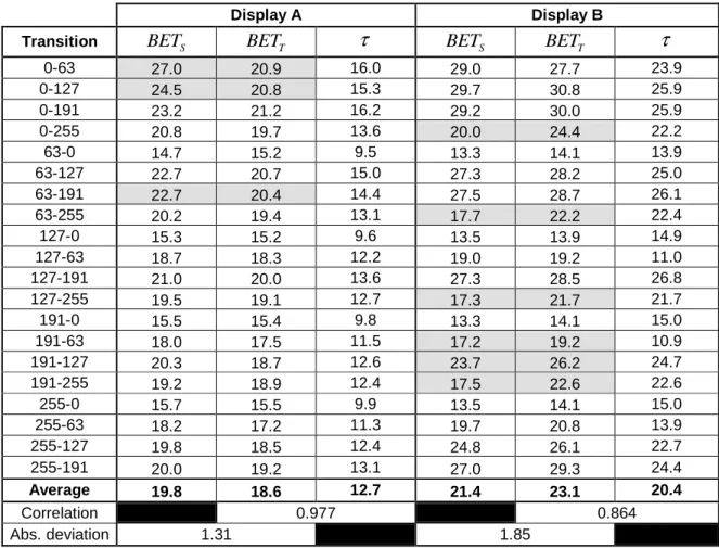
Table 2 and Table 3 present the blurred edge time values BET (from the spatial measurements) S
and BET (from the temporal step-response measurements) for each transition and each display. T
The response time τ has been computed as well from the temporal step-response measurements. The average value of these three measures is specified. The tables also present the correlation between BET and T τ for each display, as well as the absolute deviation between BET and S
T
Display A Display B
Transition BETS BETT τ BETS BETT τ
0-63 27.0 20.9 16.0 29.0 27.7 23.9 0-127 24.5 20.8 15.3 29.7 30.8 25.9 0-191 23.2 21.2 16.2 29.2 30.0 25.9 0-255 20.8 19.7 13.6 20.0 24.4 22.2 63-0 14.7 15.2 9.5 13.3 14.1 13.9 63-127 22.7 20.7 15.0 27.3 28.2 25.0 63-191 22.7 20.4 14.4 27.5 28.7 26.1 63-255 20.2 19.4 13.1 17.7 22.2 22.4 127-0 15.3 15.2 9.6 13.5 13.9 14.9 127-63 18.7 18.3 12.2 19.0 19.2 11.0 127-191 21.0 20.0 13.6 27.3 28.5 26.8 127-255 19.5 19.1 12.7 17.3 21.7 21.7 191-0 15.5 15.4 9.8 13.3 14.1 15.0 191-63 18.0 17.5 11.5 17.2 19.2 10.9 191-127 20.3 18.7 12.6 23.7 26.2 24.7 191-255 19.2 18.9 12.4 17.5 22.6 22.6 255-0 15.7 15.5 9.9 13.5 14.1 15.0 255-63 18.2 17.2 11.3 19.7 20.8 13.9 255-127 19.8 18.5 12.4 24.8 26.1 22.7 255-191 20.0 19.2 13.1 27.0 29.3 24.4 Average 19.8 18.6 12.7 21.4 23.1 20.4 Correlation 0.977 0.864 Abs. deviation 1.31 1.85
Table 2: Measurement results for displays A and B. Time values are expressed in milliseconds. The correlation between
T
BET and τ is given as well as the absolute deviation between the blurred edge time obtained with spatial
measurements BETS and the blurred edge time obtained with temporal measurements BETT. Shaded cells correspond to BET values for which there is more than 10% difference between one method and the other.
It can be first observed that the values of response times are far from those given by manufacturers. As expected, displays with backlight flashing (C and D) have lower BET values although their response time τ is quite high. It is interesting to observe that for displays without motion-blur reduction method (A and B) BET and τ are correlated. On the contrary, for displays with backlight flashing, both values seem to vary inversely: the higher BET values were obtained for transitions with low response time. If we compare displays, we can observe that
display A has a response time which is on average 28% lower than the one of display C, whereas the motion blur width is 29% higher than on display C.
Display C Display D
Transition BETS BETT τ BETS BETT τ
0-63 13.0 14.2 18.1 13.7 14.1 22.2 0-127 15.5 14.3 22.3 15.5 15.0 21.0 0-191 14.3 15.2 21.8 13.8 13.0 20.9 0-255 13.5 13.9 18.7 15.7 15.6 9.7 63-0 15.2 15.7 17.4 14.7 14.3 9.5 63-127 12.8 13.7 24.8 14.3 13.9 22.6 63-191 13.5 14.1 21.4 14.2 14.0 20.8 63-255 13.7 13.7 18.4 15.2 15.5 9.6 127-0 15.8 15.6 9.4 15.8 15.2 9.5 127-63 15.3 14.7 10.7 15.8 15.2 9.9 127-191 12.3 13.0 24.4 12.7 13.1 22.4 127-255 13.2 13.3 18.8 15.3 15.4 9.4 191-0 15.5 15.7 10.0 15.2 15.4 9.7 191-63 15.7 15.3 9.6 15.7 15.6 10.2 191-127 13.8 14.2 21.2 15.3 14.9 17.7 191-255 13.0 12.6 22.4 14.8 15.4 9.4 255-0 16.3 16.1 10.7 15.2 15.7 10.0 255-63 15.8 15.6 9.9 16.0 15.9 10.3 255-127 14.8 14.7 19.1 15.2 15.3 10.2 255-191 12.5 12.7 23.6 13.2 14.0 21.1 Average 14.3 14.4 17.6 14.9 14.8 14.3 Correlation -0.762 -0.817 Abs. deviation 0.47 0.39
Table 3: Idem as Table 2 for displays C and D.
These observations confirm that the response time is not sufficient to characterize motion blur and even worse some wrong conclusions can be drawn. Actually, since their temporal step-response is modified to approach an impulse-type step-response, in order to reduce motion blur, it seems to be not suitable to measure classical response time of displays using backlight flashing. Some significant differences are observed between the results of the two measurement methods. These differences are particularly important for display B (with an absolute deviation of 1.85 ms) due to the residuals of the PWM present on the blurred edge profile obtained from the temporal
step-responses. On display A, the more important differences occur for transitions 0→63 and 0→127; other transitions obtained quite similar results. On displays C and D, despite of high temporal modulations due to backlight flashing, results are very similar with an absolute deviation less than 0.5 ms. This is quite surprising, especially for display C on which some residuals of the backlight modulations are present.
As a whole, BET values obtained from both methods (on the 4 displays and for 20 gray-to-gray transitions) are quite well correlated. The linear correlation coefficient between BET and T BET S
is 0.940 and the absolute deviation between both set of values is 1.03 ms, which is 6% of the mean value.
6 Discussion
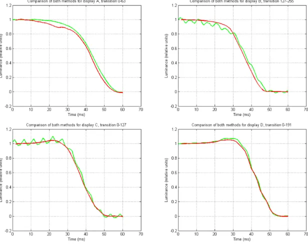
Observation of the obtained results shows some discrepancies between both measurement methods, especially for display B. Figure 9 compares the blurred edge profiles obtained with both methods. For each display, we plot the blurred edge profile for a gray-to-gray transition on which the BET variation was important. Several reasons can explain the differences in the measurement of BET .
First of all, some temporal artifacts can appear on the blurred edge profiles obtained by convolution of the temporal step-responses with a window of one-frame-period width (green curves). This is particularly obvious for displays B and C. These temporal artifacts are the residuals of the temporal modulations present on the displays step-responses. These modulations are due to pulse-width-modulation circuit for backlight dimming in the case of display B, and due to the backlight flashing system for motion-blur reduction in the case of display C. They are not filtered out by the convolution because their frequencies are not a multiple of the display refresh
frequency (PWM driving frequency is 204 Hz on display B, BF frequency is 192 Hz on display C). Actually, the convolution with a window of one-frame-period width permits us to remove from the step-response spectrum the display refresh frequency as well as all multiples of it (the spectrum is multiplied with a sinc function which have zero-crossings at nonzero multiples of the
display refresh frequency). For this reason, temporal residuals are not observed on the blurred edge profiles of display D: the frequency of the backlight flashing system of this display is 180 Hz, a multiple of the display refresh frequency 60 Hz. On displays B and C, temporal modulations are only attenuated but not totally removed. M. E. Becker [1] and X. Feng et al. [3]
have performed similar measurements on a display with a PWM driving. They obtained very clean blurred edge profiles because the PWM frequency was a multiple of the display refresh frequency (225 Hz / 75 Hz in the first case, 120 Hz / 60 Hz in the second). However, it is important to be aware that if the PWM driving frequency is not a multiple of the display refresh frequency, some residuals will be present on the blurred edge profile. The amplitude of these residuals was not very high in our case but they can potentially affect the measurement of the blurred edge time and it might, therefore, be necessary to filter them. However, camera measurements provide very clean results due to the longer temporal integration performed by the sensor. Moreover, the temporal summation of camera frames to obtain the blurred edge profile also participates to the reduction of these temporal variations.
Differences in the results obtained from both measurement methods can also come from camera measurements. On display A for example (cf. Figure 9), for which there is no temporal issues on the step-responses, an important discrepancy occurs for low luminance transitions (particularly 0→63 and 0→127) because at low luminance, camera frames could be quite noisy. Moreover, the small luminance difference between two gray levels (especially on display A which was the one with the lowest peak luminance, cf. Table 1) can intensify the noise effects.
Finally, considering measurements results, we can summarize the following statements about the two measurements methods.
Concerning the temporal measurements:
• They are considered more accurate due to higher sampling rate, and they do not require any image processing or motion compensation.
• They are easier to carry out and reproducible from one lab to another.
• In the case of PWM or BF with a frequency that is not a multiple of the display refresh frequency; blurred edge profiles obtained from temporal measurement contain some temporal residuals that can affect the BET computation. These residuals may be necessary to be filtered out. This could introduce variations from one lab to another. Concerning the camera measurements:
• They need more complicated apparatus and require much time for the measurements as well as for data processing afterwards.
• They are less sensitive to the temporal modulations of PWM driving circuits or BF systems and give clean blurred edge profiles.
Figure 9: Comparison of the two measurement methods on each display, for a gray-to-gray transition on which variation is important. Transition 0→63 for display A, transition 127→255 for display B, transition 0→127 for display C, and transition 0→191 for display D. The green profiles are obtained from temporal step-responses; the red ones are obtained
from camera measurements.
7 Conclusion
In this paper, we presented some results of motion blur measurements on LC displays. Two methods have been used to obtain blurred edge profiles. First one used a stationary high-speed camera to picture the moving edge. Second one consists in the convolution of the temporal step-response of the display with a one-frame-period wide window. Measured blur indexes have been compared between them and with the response time.
These measurements confirm that the blurred edge time can be obtained from classical temporal step-response measurements [1] [3] [15] even for liquid crystal displays with impulse-type
improvements such as backlight flashing. There is a very good correlation between results obtained from both approaches, with an absolute deviation less than 6% of the mean value over the 20 transitions measured on four displays.
However, some differences have been pointed out between both approaches. The main issue occurs with temporal measurements: temporal modulations due to pulse-width-modulation driving circuit and backlight flashing systems can lead to important discrepancies in the blurred edge profiles if the frequency of these modulations is not a multiple of the display refresh frequency. This is an important finding since it has not been highlighted in recent works on the topic [1] [3]. Some errors can also occur with the spatial measurements: grabbed frames could be quite noisy especially for low luminance transitions.
The measurement method using temporal step-responses might be more precise due to high sampling rate, and it is easier to carry out regarding instrumentation and procedure. As a result, if the temporal step-responses do not contain temporal modulations or if these modulations have a frequency which is a multiple of the display refresh frequency, this approach seems to be a good alternative to high speed camera measurements. Of course, the temporal residuals, if any, could also be filtered afterwards, but this could lead to additional approximations and variations. On the other hand, camera measurements need more expensive apparatus and procedures, and they are more time-consuming. However, they permit us to obtain clean blurred edge profiles, disregarding the noise issues at low luminance levels.
This work is only a first step in the estimation of the perceived motion blur on LCD. In order to determine acceptable levels and temporal requirements for liquid-crystal displays, studies will follow that deal with the subjective perception of motion blur, inspired by existing works on this aspect [11] [12] [16].
8 Acknowledgement
This work has been financed by TCO Development and VINNOVA (The Swedish Governmental Agency for Innovation Systems), which is hereby gratefully acknowledged. It has also been supported by the French région Pays de la Loire.
The authors would also like to thank Intertek Semko Sweden for their assistance in the study.
9 References
[1] M. E. Becker, "Motion-blur evaluation: A comparison of approaches", Journal of the SID, Vol.16, 10, pp. 989-1000, 2008.
[2] D. H. Brainard, "The Psychophysics Toolbox", Spatial Vision 10(4), pp. 433-436, 1997.
[3] X. F. Feng, H. Pan, and S. Daly, "Comparisons of motion-blur assessment strategies for newly emergent LCD and backlight driving technologies", Journal of the SID, Vol.16, 10, pp. 981-988, 2008.
[4] M. A. Klompenhouwer, "Temporal impulse response and bandwidth of displays in relation to motion blur", SID Symposium Digest, Vol. 36, pp. 1578-1581, 2005.
[5] T. Kurita, “Moving picture quality improvement for hold-type AM-LCDs”, SID Symposium Digest, Vol. 32, pp. 986-989, 2001.
[6] X. Li, X. Yang, and K. Teunissen, "LCD motion artifact determination using simulation methods", SID Symposium Digest, 37, pp. 6-9, June 2006.
[7] K. Oka and Y. Enami, “Moving picture response time (MPRT) measurement system”, in SID Symposium Digest, Vol. 35, pp. 1266-1269, 2004.
[8] H. Pan, X.-F. Feng, and S. Daly, "LCD motion blur modeling and analysis", IEEE International Conference on Image Processing, ICIP 2005, 2, pp. 21-24, September 2005.
[9] D. A. Robinson, “The mechanics of human smooth pursuit eye movement”, Journal of Physiology, 180, pp. 569-591, 1965.
SID, Vol. 14, 8, pp. 681-686, 2006.
[11] J. Someya and H. Sugiura, “Evaluation of liquid-crystal-display motion blur with moving-picture response time and human perception”, Journal of the SID, Vol. 15, 1, pp. 79-86, 2007.
[12] W. Song, X. Li, Y. Zhang, Y. Qi and X. Yang, “Motion-blur characterization on liquid-crystal displays”, Journal of the SID, Vol. 16, 5, pp.587-593, 2008.
[13] TCO Development AB, "TCO'06 Media Displays", Tech. Rep. TCOF1076 version 1.2, Stockholm, Sweden, 2006.
[14] VESA, "Flat Panel Display Measurements", Tech. Rep. Version 2.0, Video Electronics Standards Association, 2005.
[15] A. B. Watson, "The Spatial Standard Observer: A human vision model for display inspection", SID Symposium Digest, 37, pp. 1312-1315, 2006.
[16] T. Yamamoto, S. Sasaki, Y. Igarashi and Y. Tanaka, “Guiding principles for high-quality moving picture in LCD TVs”, Journal of the SID, Vol. 14, 10, pp. 933-940, 2006.