HAL Id: hal-02167082
https://hal.archives-ouvertes.fr/hal-02167082
Submitted on 28 Jun 2019
HAL is a multi-disciplinary open access
archive for the deposit and dissemination of
sci-entific research documents, whether they are
pub-lished or not. The documents may come from
teaching and research institutions in France or
abroad, or from public or private research centers.
L’archive ouverte pluridisciplinaire HAL, est
destinée au dépôt et à la diffusion de documents
scientifiques de niveau recherche, publiés ou non,
émanant des établissements d’enseignement et de
recherche français ou étrangers, des laboratoires
publics ou privés.
Autonomous, Short range Communication device
Ammar Ahmed, Jean-François Diouris, Jean-Yves Baudais
To cite this version:
Ammar Ahmed, Jean-François Diouris, Jean-Yves Baudais. Autonomous, Short range Communication
device. Fifth Sino-French Workshop on Information and Communication Technologies (SIFWICT
2019), Jun 2019, Nantes, France. �hal-02167082�
Fifth Sino-French Workshop on Information and Communication Technologies SIFWICT 2019 - June 21, 2019, Nantes, France
Autonomous, Short range Communication device
AMMAR AHMED
University of Nantes CNRS - IETR Nantes, France [email protected]J.F.DIOURIS
University of Nantes CNRS - IETR Nantes, France [email protected]J.Y.BAUDAIS
CNRS - IETR Rennes, France [email protected]Abstract—We consider an application where we want to determine the orientation of a battery-less device (a dice). The passive system is supplied with power and the communication is obtain through the change of the load, providing a short range autonomous communication and power transfer. Modeling of such system is crucial for the analysis of the task for the detection of the orientation with or without the need of sensor. The energy harvesting is one of the crucial step in achieving the goal of the such system and it is important to determine the impact of parameters such as distance, current and size in the system.
Index Terms—wireless power transfer, magnetic field density, coupling factor, resonance frequency.
I. INTRODUCTION
The first wireless power transfer (WPT) application devel-opment by Nikola tesla [1] opened new doors for transferring power. This technology was not explored during that time but since the past decade it has attracted a lot of attention. Since the integration of WPT in mobile phones, a lot of research is being done in the context of IOT. One of major application of WPT is wireless and non-invasive transfer of power to the pace makers permanently embedded on the patient’s heart. Further applications are explored to apply such principle and enhance the ease and automation of connected objects.
This paper explores another application of wireless power transfer, which could be utilized in other applications as per need. The application is a simple dice game, in which the dice is thrown on to the table and the orientation of the dice is determined. A similar application was presented in [6] [7] which utilizes an RFID based system, and comprises an accelerometer sensor for the detection of orientation. The reading range in [6] is very small and the reader has to be brought near to the dice for each roll of the dice. The approach presented in this paper utilities magnetic coupling between two coils for power transfer as well as the detection of the orientation. The dice is a passive object and does not contain any on board power source. The power is supplied through the magnetic coupling. The transmitter coil transmits the energy, which is embedded in the board of the dice game, to the receiver coil in the dice. The orientation is determined by utilizing the load on the side of the orientation. For the correct determination of the orientation of the dice the amount of energy received should be determined.
The next section explores the model of the system under consideration. Then the model is validated by the practical implementation and a comparison is made.
II. MODEL OF THE APPLICATION
A. The Two coil Wireless power transfer system
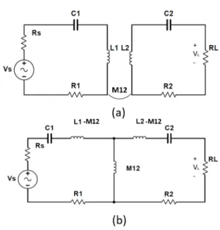
In this section the simple two coil power transfer system [3] is analyzed as shown in the Fig. 1. M12 is the mutual
inductance which is given by the relation.
M12= k
p
L1L2 (1)
Where k is the coupling factor between two coils.
Fig. 1. (a) Two coil power transfer system (b) Equivalent T-model
I1 and I2 represents the current in the transmitter coil and
receiver coil respectively which are defined in (5)and (6). VS
is the source voltage and VL is the load voltage across the
load RL, the ratio is given in (4). Z1 (2) and Z2 (3) are the
cumulative impedances at Tx and Rx coils.
Z1= RS+ R1+ jωL1+ 1 jωC1 (2) Z2= RL+ R2+ jωL2+ 1 jωC2 (3) VL VS = jωM12RL Z1Z2+ (ωM12)2 (4)
I1= Z2VS Z1Z2+ (ωM12)2 (5) I2= jωM12VS Z1Z2+ (ωM12)2 (6) Here, ωis the pulsation of the circuit.
B. Magnetic field density
To have a comprehensive analysis of the power harvesting, the first step is to determine the magnetic field density gen-erated from the transmitter coil at different point. Since, the amount of magnetic field density will determine the amount of power received at the receiver coil. The model presented by [2] is utilized in this study which is also the basis of [5]. It follows the basic equations of Weber and then the geometry of the coil is taking into account to determine the magnetic field density.
Fig. 2. Magnetic field density at point P
Bx= − ∂Ax ∂z , By= − ∂Ax ∂z , Bx= ∂Ay ∂x − ∂Ax ∂y (7) Ax= µ0I1 4π ln[ (r1+ a + x) (r2− a + x) .(r3− a + x) (r4+ a + x) ] (8) Ay= µ0I1 4π ln[ (r2+ b + y − s) (r3− b + y − s) .(r3− b + y − s) (r4+ b + y − s) ] (9) After putting (8) and (9) in (7) and taking derivatives we obtain the formula for the magnetic field density and a more computer program oriented formula :
Bz= µ0I1 4π 4 X a=1 [ (−1) αd α rα[rα+ (−1)α+1Cα] − Cα rα(rα+ dα) ] (10) Bx= µ0I1 4π 4 X a=1 [ (−1) α+1z rα(rα+ dα) ] (11) By= µ0I1 4π 4 X a=1 [ (−1) α+1z rα[rα+ (−1)α+1Cα] ] (12)
Bx,By and Bzare the magnetic field density at a point due
coming from each direction. For multiple turn coil, the (10), (11) and (12) are multiplied by number of turns. Also, here r1, r2, r3 and r4 are the distances to the point P(x,y,z) from
each corner as shown in the Fig. 2 and are defined as : r1= p (a + x)2+ (y + b − s)2+ z2 r2= p (a − x)2+ (y + b − s)2+ z2 r3= p (a − x)2+ (y − b − s)2+ z2 r2= p (a + x)2+ (y − b − s)2+ z2 and, C1= −C4= a + x, C2= −C3= a − x d1= d2= y + b − s, d3= d4= y − b − s
Where s represents the displacement from the center on the Y-axis. The total magnetic field density in each direction (13) and the magnitude is given by (14)
B = Bxi + Byj + Bzk (13)
kBk =qB2
x+ By2+ Bz2 (14)
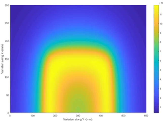
For this particular application we simulated the behavior of the magnetic field density generated by the transmitter coil which is shown in Fig. 3 and Fig. 4. This relation is further used to estimate the induced voltage in the further section.
Fig. 4. Magnetic field density generated by rectangular coil (Top view).
C. Determining Mutual Inductance
Mutual inductance (1) of rectangular coil is different from circular coil. To determine the coupling factor, an analytic model [4] is considered and coupling factor of a single coil is calculated as shown in the Fig. 5 and then number of turns of transmitter and receiver coils are integrated to calculate the total mutual inductance, which is as follows. The magnetic flux is determined for each side of the coil using Biot-Savart law. φij= Z Sj Bi.dSj = Z Sj Biz.dSj= Z Sj B.cosθ.dSj (15)
We can solve this equation by taking one side each at a time and then sum all the results to get the desired mutual inductance. The BCD-zcalculation is given as:
φCD−z = Z dj −dj dy Z cj −cj BCD−zdx (16) φCD−z = µ0 2pi[ q (bi+ dj)2+ z2+ (ai+ cj)2 − (ai+ cj).arctanh ai+ cj p(bi+ dj)2+ z2+ (ai+ cj)2 −q(bi+ dj)2+ z2+ (ai− cj)2 + (ai− cj).arctanh (ai− cj) p(bi+ dj)2+ z2+ (ai− cj)2 −q(bi− dj)2+ z2+ (ai+ cj)2 + (ai+ cj).arctanh ai+ cj p(bi− dj)2+ z2+ (ai+ cj)2 + q (bi− dj)2+ z2+ (ai− cj)2 −(ai− cj).arctanh ai− cj p(bi− dj)2+ z2+ (ai− cj)2 ] (17)
Here we have the flux produced by one side and the contribution of the remaining sides can be calculated as shown in Fig. 5. To calculate the remaining three sides the similar methodology can be applied and then by replacing aiwith bi,
and cj with djin equation to get φBC-z.
Fig. 5. Rectangular Tx and Rx coils.
Also, we have φAB-z= φCD-zand φDA-z= φBC-z. The overall
magnetic flux is given by.
φij= φAB-z+ φCD-z+ φDA-z+ φBC-z
Hence, the mutual inductance is given by Mij = φij. For the
multiple number of turns of transmitter NT and receiver coil
NR, the total mutual inductance is given as
M = NT X i=1 NR X i=1 Mij (18)
III. EXPERIMENTALRESULTS
To calculate the voltage induced in the receiver coil, across the load resistance we need to take into account other param-eters such as quality factor (Q), Resonance frequency (f0) and
the area of the receiver coil (S).
f0= 1 2π√LC (19) Q = 1 R r L C (20)
The output voltage is defined as :
V0= 2πf0QSB0cosα (21)
The voltage induced is directly proportional to the angle of the arriving signal and the angle of the receiver antenna
coil. The maximum voltage is induced when the coil is perpendicular to the arriving magnetic field where α= 0. The Fig. 6 and Fig. 7 represents the amount of voltage induced from center of the coil to the both ends of the coil in the horizontal axis and the upper half of the vertical axis, keeping the distance between the the coils constant. The similarity between magnetic field density and induced voltages could be seen, as they have quite similar curves.
Fig. 6. Voltages induced in the receiver coil.
Fig. 7. Voltages induced in the receiver coil (Top view).
The experimental setup in Fig. 8 was used to validate the results. The results obtained are shown in the Fig. 9. The measured values were taken at receiver coil at the height of 4.5 cm from the surface of the transmitter coil. The two curves are not matched exactly in the Fig. 9, the relative error is accounted to be around 20 percent, which could be reduced while operating at a lower height and optimizing certain parameters in Table I. The experimental results are
TABLE I
PARAMETERS USED IN THE EXPERIMENTAL SETUP. Parameter Values Parameters Values
Rs 50 Ω RL 120 Ω
L1 3.2 mH L2 290 µH
C1 0.52 nF C2 5.868 nF
R1 120 Ω R2 50 Ω
z 4.5 cm f0 122 kHz
taken by fixing the x and z -axis and the variation of the receiver coil along the y-axis.
Fig. 8. Tx and Rx coil used in experiment.
Fig. 9. Calculated and measured induced voltages.
CONCLUSION
In this preliminary work we have modeled the transmission of power between two coils, designed for a dice game appli-cation. In next work we will see the possibility to determine the dice orientation with this system. Further results will be presented during the conference.
REFERENCES
[1] Tesla, Nikola. ”Apparatus for transmitting electrical energy.” U.S. Patent No. 1,119,732. 1 Dec. 1914.
[2] Misakian, Martin. (2000). Equations for the Magnetic Field Produced by One or More Rectangular Loops of Wire in the Same Plane. Journal of Research of the National Institute of Standards and Technology. 105. 10.6028/jres.105.045.
[3] Y. Cao and J. A. A. Qahouq, ”Evaluation of maximum system efficiency and maximum output power in two-coil wireless power transfer system by using modeling and experimental results,” 2017 IEEE Applied Power Electronics Conference and Exposition (APEC), Tampa, FL, 2017, pp. 1625-1631.
[4] Y. Cheng and Y. Shu, ”A New Analytical Calculation of the Mutual In-ductance of the Coaxial Spiral Rectangular Coils,” in IEEE Transactions on Magnetics, vol. 50, no. 4, pp. 1-6, April 2014, Art no. 7026806. [5] Mochol´ı Belenguer, Ferran Salcedo, Antonio Mili´an, V´ıctor
Arroyo-Nunez, Jose. (2018). Double Magnetic Loop and Methods for Calcu-lating Its Inductance. Journal of Advanced Transportation. 2018. 1-15. [6] S. Sasaki, T. Seki and S. Sugiyama, ”Batteryless Accelerometer Using
Power Feeding System of RFID,” 2006 SICE-ICASE International Joint Conference, Busan, 2006, pp. 3567-3570.
[7] S. Sasaki et al., ”Batteryless-Wireless MEMS Sensor System with a 3D Loop Antenna,” SENSORS, 2007 IEEE, Atlanta, GA, 2007, pp. 252-255.