Radial tree-growth modelling with fuzzy
regression
J.J. Boreux, C. Gadbin-Henry, J. Guiot, and L. Tessier
Abstract: A so-called fuzzy linear regression is used in dendroecology to model empirically tree growth as a function of a bioclimatic index representing the water stress, i.e., the ratio of actual evapotranspiration to potential
evapotranspiration. The response function predicts tree growth as (fuzzy) intervals, narrow in the domain where the bioclimatic index is most limiting and becoming progressively larger elsewhere. The method is tested with a population of Pinus pinea L. from the Provence region in France. It is shown that fuzzy linear regression gives results comparable with those obtained using a linear response function. The interval of credibility given by the fuzzy regression suggests that more precise expected growth is obtained for high water stress, which is typical of Mediterranean climate. Fuzzy linear regression can be also a method to test different hypotheses on several potential predictors when any further experimental approach is quite impossible as it is for trees in their natural environment. To sum up, fuzzy regression could be a first step before the construction of a kind of growth simulator adapted to different environments of a given species. In environmental sciences, the fuzzy response function thus appears to be an approach between the
mechanistic and the statistical descriptive approaches.
Résumé : Une régression dite linéaire floue est utilisée en dendroécologie pour modéliser empiriquement la croissance des arbres en fonction d’un indice bioclimatique représentant le stress hydrique, c’est-à-dire, le ratio de
l’évapotranspiration réelle par rapport à l’évapotranspiration potentielle. La fonction prédit la croissance des arbres par intervalles (flous) qui sont étroits dans la région où l’indice bioclimatique est le plus limitatif et s’élargissent
progressivement dans les autres régions. La méthode est testée avec une population de Pinus pinea L. de la région provençale de France. Il est démontré que la régression linéaire floue donne des résultats comparables à ceux obtenus avec une fonction à réponse linéaire. L’intervalle de crédibilité donné par la régression floue suggère une croissance plus precise attendue lors d’un stress hydrique élevé, typique du climat méditerranéen. La régression linéaire floue peut aussi servir à tester différentes hypothèses au sujet de prédicteurs potentiels lorsque toute approche expérimentale additionnelle est impossible, comme dans le cas des arbres dans leur environnement naturel. En conclusion, la régression floue pourrait constituer une première étape avant la construction d’une sorte de « simulateur de
croissance » adapté aux différents milieux occupés par une espèce donnée. En sciences environnementales, la fonction de réponse floue semble donc être une approche qui se situe entre l’approche déterministe et l’approche des statistiques descriptives. Boreux et al. 1260
Empirical statistical models (Fritts 1976) usually describe
the response of tree growth to climate. Not all climate
fac-tors are important to a tree at any given moment. Only those
that limit some process can affect growth (Fritts 1982). The
principle of limiting factors states that each process is
gov-erned by one factor at a time, namely, the factor that is the
most stressing at that time. However, as we want to calculate
response functions valid for the whole live tree, it is
neces-sary to take into account a large number of possible limiting
factors and thus to use multivariate statistics.
Since the pioneer paper of Fritts et al. (1971), monthly
mean temperature and monthly precipitation over a period
from 12 to 16 months before the end of the growth, i.e.,
Au-gust or September depending on the species and (or) the
cli-mate, are used as growth predictors. As such a large number
of predictors is not without statistical problems (correlation
of the predictors, reduced number of degrees of freedom,
etc.); the set is reduced to independent variables by using
principal component analysis (Fritts et al. 1971; Fritts 1976;
Guiot et al. 1982a). The effects of using an excessively large
number of predictors have been well established by Monte
Carlo methods (Cropper 1982) or bootstrap ones (Guiot 1989).
Regrouping individual months into biological seasons
ac-cording to some a priori knowledge of the tree ecology or on
the basis of monthly response functions has also been tested
to reduce the number of parameters in the models (Guiot et
al. 1982b). More bioclimatic parameters, such as
evapotran-spiration, have also been introduced (Badeau et al. 1995; Bert
1992; Gadbin-Henry 1994 ; Lebourgeois 1995). Mechanistic
models (Shashkin and Fritts 1995) are much more difficult
to implement. In particular, the need for daily values as
Received December 22, 1997. Accepted May 17, 1998.J.J. Boreux. Fondation universitaire luxembourgeoise, avenue de Longwy, 185, 6700 Arlon, Belgique. e-mail:
C. Gadbin-Henry, J. Guiot,1and L. Tessier. Institut
méditerranéen d’écologie et paléoécologie, Centre national de la recherche scientifique, Faculté de St-Jérôme, case 451, 13397 Marseille Cédex 20, France. e-mail:
input into such bioclimatic or mechanistic models is difficult
to satisfy most of the time.
Mechanistic models should be the favoured approach in
the future, as they are the only ones to completely take into
account the biology of the problem, thus insuring a greater
robustness of the predictions. Here we do not propose such a
model, but we stay at a more empirical level, which is the
easiest approach when large sets of data, as available in
dendroecology, must be analysed. Meanwhile, by trying to
incorporate maximum a priori information into the model,
we think that more useful predictive models can be
elabo-rated. Bayesian or fuzzy logic methods are able to satisfy
these requirements, either by estimating the model
parame-ters from an a priori distribution (Bayesian approach) or by
chosing a reference point where the knowledge is maximum
and (or) by defining the shape of the fuzzy numbers
accord-ing some biological considerations.
We test a so-called fuzzy linear regression on selected
bioclimatic variables that take into account the uncertainties
inevitable in most of the data. We also show that this
ap-proach is able to take into account the particular profile of
the climatic effect on tree growth. The trees react to climate
according to the limiting factor principle, which means that
high values of the climatic factor do not have the same
pro-portional effect as low values. It also means that this
limit-ing factor can change durlimit-ing yearly tree growth and from
one year to the next.
The method is illustrated by a population of Pinus
pinea L. from the Provence region in France.
Field site
A population of Pinus pinea L. has been retained for this study, because it grows in an healthy and large stand with an active re-generation, so it is able to reflect the average ecological conditions for this species. The sensitivity to climatic variations (called “mean sensitivity” by Douglass (1936) and denoted S) has a high level for a Mediterranean species (S = 0.26).
The site is located at an altitude of 105 m, on an almost flat area near the small town of Vidauban, in the so-called Bois de Rouquan locality (43°22′N, 6°27′E). The substratum is a sandstone outcrop of the Permian depression along the crystalline massif of the Maures. In such edaphic conditions, the main limiting climatic fac-tor is humidity; this was demonstrated previously by comparing the radial growth of Pinus pinea L. with both precipitation and bioclimatic coefficients such as real or potential evapotranspiration (Gadbin-Henry 1994).
Mediterranean-type climate prevails in the studied region char-acterized by a cold winter and a warm and dry summer. The aridity coefficient of Emberger (1930) at the nearest meteorological sta-tion classifies the site in the subhumid zone, with a total annual precipitation of 889 mm, a mean annual temperature of 14.6°C, a mean minimum value of 1.7°C for the coldest month, and a mean maximum value of 30.9°C for the warmest month.
The dominant trees were retained, because they were less af-fected by competition processes and thus were the best climate re-corders (Schweingruber et al. 1990). Within this population, 14 dominant trees were selected to obtain the longest possible tree-ring series, undisturbed by any accidental event. The raw data were provided by cores obtained with the Pressler borer (three samples per tree at 60° intervals around the trunk). Tree-ring width, reflect-ing tree growth, were directly measured on planed cores with a tree-ring measuring system including integral recording.
Compari-son of ring-width chronologies revealed a mean correlation of 0.95. The whole population is represented by the mean chronology, including the 42 elementary chronologies.
Meteorological data for the period 1950–1985 (monthly precipi-tation and temperature) were provided by the nearest meteorologi-cal station having similar geographical and climatological characteristics (Fréjus; 43°26′N, 6°45′E, altitude 50 m).
Bioclimatic variables
We use three bioclimatic variables representing the water stress, winter frost, and thermal energy available in the growing season. These variables are derived from three monthly parameters easily available at a reasonable distance (40 km) from the tree-ring site analysed, i.e., the 12 monthly mean temperatures (°C), monthly precipitation amount (mm), and the monthly sunshine. Using the simple equations described in Harrison et al. (1993) and Prentice et al. (1993), these basic variables are transformed, for each year, into (i) the mean temperature of the coldest month (Tc in °C); (ii) the growing degree-days above 5°C (GDD5 in degree-days); and (iii) the ratio of actual evapotranspiration to potential evapotran-spiration (αin %).
As often, daily temperatures are not available for local meteoro-logical stations, we have devised a method to roughly calculate them from monthly values by cubic-spline interpolation. GDD5is ob-tained from these quasi-daily values by summing the part above 5°C.
For the actual evapotranspiration, a simple water-balance model is used (Harrison et al. 1993). The actual evapotranspiration (AET) is taken to be the lesser of a supply function proportional to soil moisture (Federer 1982) and a demand function set equal to the po-tential evapotranspiration (PET). PET is empirically defined as a function of the net radiation and temperature (Jarvis and Mac-naughton 1986). Net radiation is obtained as a semi-empirical function of insolation, sunshine proportion, and temperature and varies sinusoidally during the day, allowing daily actual and poten-tial evapotranspiration to be obtained by integration (Prentice et al. 1992, 1993). Sunshine is indexed as a proportion of the maximum possible sunshine hours for the latitude and month under consider-ation. In addition to the three monthly climatic variables, latitude of the site and orbital parameters (eccentricity, obliquity, and phase angle indicating the timing of the perihelion relative to the equi-noxes) are used as input variables. This method of calculatingαis rather rough, but various tests (Gadbin-Henry 1994) have shown that this approximated parameter correlates well with the studied tree-growth series.
The model requires daily precipitation values, which are ob-tained by dividing the monthly precipitation by the number of days in the month. The soil moisture,Ω, is obtained from January 1 to December 31 by integrating daily values calculated by adding the difference between daily precipitation and daily PET within a range [0, Ωmax]. Ωmax is the soil water-holding capacity above which the water runs off. As no data are available for the year prior to the study, we start with a value ofΩequal toΩmax, and for the following years, we start with the last value calculated for the previous year.
Response function using a bootstrap multiple regression
In dendroecology, it is usual to calculate the effect of climate on tree growth by a multiple regression, called a response function. This model often includes 24 predictors and sometimes more (Fritts 1976). It can be written as follows:[1]
Y
i jX
j m ij i=
+
+
=∑
β
0β
ε
1where Yiis the value of the response in the ith observation;β0and
the predictors in the ith observation, andeiis a random error term
with mean E(ei) = 0 and varianceσ2(ei) =σ2, the covariance for all
i and k; i≠k.
We know that a “good model” respects two principles: parsi-mony of parameters and small deviations between observations and predictions (Bernier 1987). On one hand, the sophisticated models (i.e., the models having a lot of parameters) adjust well to any data set but often offer poor physical meaning. On the other hand, although they can delude when they are compared with ob-servations, the sophisticated models may fail as soon as their out-put is quantitatively compared with an observation set.
To illustrate this parsimony principle, a response function has first been calculated as it is usually done by multiple regression af-ter extracting principal components. The predictand is the mean tree-ring series, and the predictors are the 24 monthly climatic pa-rameters (total precipitation and mean temperature from October of the previous year to September of the current year). These 24 pre-dictors are reduced to a smaller number of principal components. To test the validity of such a complex model, we use a bootstrap method (Efron 1979, 1983), which consists in randomly selecting a
great number of calibration sets among the observations to esti-mate the model parameters and to examine their variability. The nonselected observations are used in an independent verification (Guiot 1989). The number of replications is typically between 50 and 5000 (here 1000). The standard deviations of the mean regres-sion coefficients and of the correlation estimates between predicted and actual growth are a clue of the predictive capability of the model.
Table 1 shows that the correlation is high over the calibration data set but is much smaller over the verification data set, greatly reducing the predictive capability of such a response function. The bootstrap method clearly shows that the complex model that fits the data well on the calibration sample does not provide any signif-icant correlation when it is applied to independent data; the corre-lation of 0.42 is not significant at the 95% level.
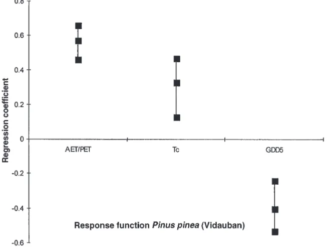
By limiting the number of predictors we want to minimize the risk of making spurious predictions. Here, only three main bio-climatic parameters described above will be used. In this Mediter-ranean region, they are, by decreasing importance, the water availability represented byα, Tc, and GDD5.
These three parameters are used in a similar bootstrap regres-sion. Table 1 shows clearly that, if the fit is apparently not as good as before on the calibration data, it is better and strongly signifi-cant on the independent data. Figure 1 shows that the tree-growth of P. pinea at Vidauban is favoured first by a highα, second by a high Tc and then a low GDD5. The negative effect of GDD5 is
likely to be also related to the summer evapotranspiration. The positive effect of Tccan be related to the limiting effect of
excep-tional low temperature in February or January.
Finally, estimates from the three bioclimatic parameters (Fig. 2) are close to the observations. The narrow error bars are certainly underestimated (because of the autocorrelation of the tree-ring se-ries). The period 1950–1971 presents a low productivity except Type of regression Calibration Verification
24 monthly variables 0.94±0.032 0.42±0.28 3 bioclimatic variables 0.76±0.071 0.66±0.17 Note: The calibration correlations were calculated from data randomly
selected for the calibration, and the verification correlations were calculated from data not used for the calibration. The bootstrap standard deviations are calculated over 1000 simulations.
Table 1. Correlation between predicted and observed tree growth using 24 or 3 climatic variables with the bootstrap standard deviations.
Fig. 1. Standardized partial regression coefficients with the 90% confidence interval between tree growth at Vidauban and three bioclimatic variables. A vertical line completely above the horizontal axis means a significant positive effect of the corresponding bioclimatic parameter on the tree growth, and a line below shows a significant negative effect.
during 1959–1961, but the discrepancies between observations and estimates show that the higher productivity is not well modelled by the climatic parameters considered. On the contrary, the period of high productivity (1972–1980), appears to be clearly explained by the combination of climatic parameters involved in the response function. This contrast shows that the response function gives only the mean behaviour of the tree in relation to the climatic variable introduced to the regression. Other factors can be invoked to ex-plain the discrepancies between data and estimates, such as the ap-proximation used in the calculation of αand the water storage in the soil during the previous year. If it appears thatαis the best ex-planatory variable, it is not easy to derive a exhaustive mechanistic interpretation from a unique response function.
Criticism of classical regression and alternative proposal
The utility of introducing another type of model is justified by the analysis of the underlying assumptions of classical regression. They are as follows (Neter et al. 1989): (i) the predictors are as-sumed to be nonrandom, although the general case where the pre-dictors are random variables can be perfectly processed by introducing new hypotheses; (ii) the random error term cannot be correlated with predictors; (iii) the random error terms are uncorrelated random variables, although this problem can be solved using methods such Durbin–Watson, ARMA, etc., which need larger samples; and (iv) as a random variable can be ajusted by using a sample, the sample size must increase with the number of predictors (data sets of at least 20 observations in the univariate case). Of course this latter constraint can be released by introduc-ing a priori knowledge.Practically, all these assumptions are never completely fulfilled. To illustrate this point, the first assumption does not hold when data result from measurements of continuous quantities (Viertl 1997). For time-series data, the third assumption is often not ap-propriate; rather, the error terms are frequently serially correlated
and lead to overestimate the model reliability. Lastly, confidence intervals estimated with few data points are too large to provide any useful information for predictive purposes. Clearly, there are many situations where the researcher should not use the classical linear regression, at least without introducing sophisticated consid-erations. Under those considerations, various other approaches have been developed, e.g., nonparametric regression techniques (kernel, local polynomial, spline.) (Fan and Gijbels 1996; Hastie and Loader 1993; Chu and Marron 1991), Bayesian methodology (Berger 1985), the Dempster–Shafer scheme (Caselton and Luo 1994), neural networks (Guiot and Tessier 1997), and fuzzy regres-sions (Tanaka et al. 1982; Heshmaty and Kandel 1985) based on the idea of fuzzy subsets (Zadeh 1973).
Fuzzy regression is a tool that has been developed to model situ-ations in which hypotheses are uncertain and data are sparse and imprecise. As explained above, the applicability of classical statis-tical tools seem to be limited under such severe conditions. For in-stance, it is very well known that the population mean, µ (unknown but assumed to be constant), can be estimated using the sample average x. Naturally, from sample to sample, we expect de-viations between sample averages x and their target µ. How do these deviations fluctuate? Classically the investigator computes a confidence interval centred on the sample average x with a radius r to which a given probability (often 95%) to include the unknown population parameter µ is assigned. In others words, in repeated sampling, the population meanµ will belong to the confidence in-terval [x ±r] 95% of the time. It must be repeated that the confi-dence interval assessment requires some assumptions seldom fulfilled in environmental sciences. Indeed, hypotheses such as random sampling or statistical independence often cannot be assumed.
So, what can the environmentalist do? He may or may not take into account the violations of assumptions. The second attitude is not only unrealistic but also leads to unreliable predictions. The Fig. 2. Actual tree growth of Pinus pinea L. at Vidauban (dots) and estimates using a bootstrap regression from three bioclimatic variables. The central line gives the median calculated over 1000 simulations, and the two other lines give the 90% confidence interval.
first attitude calls for unusual methods of which the difficulty level can be quite high for a majority of the practitioners. As an example, a Bayesian approach (Berger 1985; Bernier 1987) can of-fer robust analysis in environmental sciences; unfortunately, many environmentalists do not master it.
In others words, a skilled approach must also be workable or understandable. In this way, fuzzy techniques seem to offer a good compromise between “reliability” and “complexity.” Since fuzzy regression operates with fuzzy numbers, we have to present the es-sential of fuzzy sets.
Elementary concepts of fuzzy logic
Fuzzy logic differs from conventional logic in that it aims at providing techniques for approximate rather than precise reason-ing. Unlike classical probability, which is based on a frequency distribution in a random population, fuzzy logic deals with describ-ing the characteristics of properties. Fuzzy logic describes proper-ties that have continuously varying values by associating partitions of these values with a semantic label. The power of this approach comes from the fact that these semantic partitions can or even should overlap.
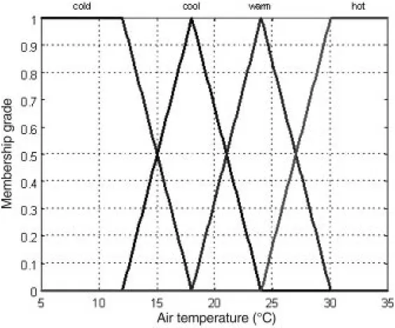
As an example, consider the parameter “air temperature.” This parameter can be broken down into four subsets: “cold,” “cool,” “warm,” and “hot.” The interval from the smallest to the largest al-lowable value is called the universe of discourse denoted X. Here X is the real interval from 5 to 35°C (Fig. 3).
Assume that the actual air temperature, say x0, is 25°C. We can see that x0belongs to the subset warm but also to the subset hot (Fig. 3). What is the difference? It lies in the so-called degree of membership. This particular value of air temperature x0= 25°C be-longs to the subset warm with a degree of truth equal to five of six, while it is only one of six for the subset hot. Moreover, x0does not
belong either to the subset cold or to the subset cool. So, the de-gree of membership of x0is equal to zero for both.
Subsets like cold, cool, warm and hot are called fuzzy subsets of X because each element x of X belongs to every subset with mem-bership grade varying between zero and one. In other words, fuzzy logic is a graduated logic based on the idea of membership func-tion from the universe of discourse X to the real interval [0,1]. Each element x of the universe of the discourse X is associated with a real number between zero and one giving its degree of truth fulfilment to the subset being considered.
As a contrast, consider binary logic. We recall that an ordinary subset, say E, is always defined with respect to some universe of discourse X, which is itself an ordinary set. Any element x of X be-longs or does not belong to the subset E, and the corresponding membership grade is one or zero; there is no place for an interme-diate membership grade. Accordingly with the wording used in fuzzy logic, an ordinary set is called a “crisp” set. To distinguish between fuzzy and crisp concepts, fuzzy subsets will be denoted with a tilde (~).
Assume A is a fuzzy subset of X with membership function~
µA(x). It must be emphasized that the universe of discourse X is a
crisp set, i.e., often the set of real numbers. On one hand, the open interval from its smallest to its largest value is called the “support” of A. On the other hand, the closed interval consisting of all ele-~ ments with membership grade one is called the “core” of the fuzzy subsetA. Some fuzzy subsets have the empty set~ ∅for core. If the core contains only one element this element is called the “pivot” of the fuzzy subset. Thus, any fuzzy subset A is completely defined~ by its membership functionµA(x), which involves both support and core.
Often, the membership functionµcan be broken down into two functions LA(x) and RA(x) corresponding to the “left” and “right” Fig. 3. Four fuzzy subsets to describe air temperature (°C). An element x in the universe of discourse X, here the real interval 5–35°C, belongs to each fuzzy subset with a degree of truth between zero and one.
sides. For instance, the fuzzy subsets cold and warm (Fig. 3, Table 2) are defined by a linear left and right function (p = q = 1).
Fuzzy numbers
Fuzzy numbers are special fuzzy subsets. AssumeA is a fuzzy~ subset of X with membership functionµA(x).A is a fuzzy number~ if and only if (i) the universe of discourse X is the set of real num-bers; (ii) at least one element x of the support has its membership grade equal to one (normal assumption, i.e., the core exists); and (iii) the membership function has no local extrema (convex assumption).
The two latter properties limit the shape that a fuzzy number can take: it is always nondecreasing to the left of the core and nonincreasing to the right of the core. So, a real number can be seen as a fuzzy number whose support comprises only one element that has a membership grade equal to one.
The simplest type of fuzzy number has a triangular or trape-zoidal membership function (Fig. 3, Table 2). It is convenient to introduce so-called left-right fuzzy numbers (LRFN) so as to be
able to deal with curvilinear membership functions (Dubois and Prade 1980).
Assume a fuzzy numberA with support ]a~ –, a+[, pivot {a}, and membership function µA(x). This latter can be broken down into LA(x) and RA(x) that have a simple analytic form:
[2]
µ
A A p Ax
L x
a
x
a
a
x
a
a
R x
x
A( )
( )
[(
) / (
)]
]
, ]
( )
[(
=
= −
−
−
∈
= −
−
− −1
1
a
) / (
a
a
)]
qAx
[ ,
a a
[
+−
∈
+0
otherwise
where both exponents pAand qAare positive real numbers giving a certain curvature to the selected membership function (Figs. 4 and 5). The subscript A in eq. 2 and anywhere in the current text refers to the fuzzy number A. It will be omitted if no confusion is~ possible.
Thus, eq. 2 defines an LRFN. Hence, any LRFN is rigorously defined with five real numbers ordered as support lower end, pivot, support upper end, left exponent, and right exponent (yielding the ~ A≡cold B~≡warm Support ]5,18[ ]18,30[ Core [5, 12] {24} (pivot) Left No L x L x x B b :[ , ] [ , ] ( ) ( )/ 18 24 0 1 18 6 → = − a Right R x R x x A B :[ , ] [ , ] ( ) ( ) / 12 18 0 1 30 6 → = − a R x R x x B B :[ , ] [ , ] ( ) ( )/ 24 30 0 1 30 6 → = − a
Table 2. Definitions of the fuzzy subsetsA~≡cold andB~≡warm.
10 12 14 16 18 20 0 0.1 0.2 0.3 0.4 0.5 0.6 0.7 0.8 0.9 1 x M e m ber s h ip gr ade h
h = 0.5
a
-hb
-ha
+hb
+hFig. 4. Any LRFN, e.g.,A~; {10, 14, 20, 0.75, 2.5}, is rigorously defined with five real numbers ordered as support lower end (a–= 10), pivot (a = 14), support upper end (a+= 20), left exponent (p = 0.75), and right exponent (q = 2.5) yielding the membership function LA(x) and RA(x) (see eq. 2). If we define a second LRFN,B~; {11, 15, 21, 0.5, 4}, the sum is defined by eq. 3; for a particular h = 0.5, it isA +~ B = [12. + 14, 18.5 + 20]~ h = 0.5.
membership function). Any LRFN A can thus be written as fol-~ lows:A~≡{a–, a, a+, pA, qA} (Fig. 4). So, the LRFN concept allows us to represent not only the data but also some of the knowledge. As shown in Fig. 5, a large value for both exponents gives a “fat” fuzzy number, because each x in its support is thought to be highly possible. In the opposite case, values less than one produce “slim” fuzzy numbers because only the elements x near the pivot are thought to be highly possible. The linear case deals with p = q = 1 (triangular fuzzy number or TFN).
An example: evapotranspiration
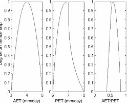
Evapotranspiration is the combined process of evaporation from both soil and plant surfaces and transpiration through plant sur-faces. The AET/PET ratio is a physically meaningful index of wa-ter availability. Estimating the AET and PET of a vegetative surface is a very difficult and time-consuming task fraught with uncertainty (Burman and Pochop 1994). For instance, AET can be achieved with a lysimetric measurement and PET can be a model output (e.g., Penman formula). In all cases, results are uncertain, and these parameters can be seen as fuzzy numbers. For example, AET is given asA~≡{a–, a, a+, pA, qA} = {3, 4, 5, 2, 2} and PET is given asB~≡{b–, b, b+, pB, qB} = {6, 7, 8, 2, 1/2} (Fig. 6).
The AET/PET ratio is obtained by dividing two fuzzy numbers, but such division is not as straightforward as with real numbers (Kaufmann and Gupta 1991).
Arithmetic operations on fuzzy numbers
Given two fuzzy numbers, any fixed membership grade h de-fines, for all he [0,1], two closed intervals of real numbers (Fig. 4). In fact, each fuzzy subset, and thus also each fuzzy number, can be fully and uniquely represented by its interval strata called h-cuts in fuzzy terminology. Therefore, arithmetic operations on fuzzy num-bers are defined in terms of arithmetic operations on their h-cuts, i.e., arithmetic operations on closed real intervals.
For short, any arithmetic operation on fuzzy numbers is per-formed for each level h for all 0≤h≤1. As the set of real numbers is linearly ordered, operations on closed real intervals are very easy using the following algorithm.
Consider two fuzzy numbers, sayA and~ B. Any level h defines~ two closed real intervals respectively noted [a–, a+]hand [b–, b+]h.
Let an asterisk denote any of the four basic arithmetic operations. The fuzzy number C =~ A*~ B is determined as follows. For all~ he [ , ]0 1 :
[3]
[c
–, c
+]
h= [a
–, a
+]
h*[b
–, b
+]
hwhere
c
–= min{a
–*b
–, a
–*b
+, a
+*b
–, a
+*b
+}
c
+= max{a
–*b
–, a
–*b
+, a
+*b
–, a
+*b
+}
with a restriction for the division that the denominator closed inter-val cannot contain zero.
As sketched in Fig. 6, the AET/PET ratio is a fuzzy number that can be approximated by the LRFN ~α = {3/8, 4/7, 5/6, ≈8/5,
≈46/25} the exponents p and q resulting from a numerical approxi-mation (not shown here). In general, arithmetic operations on fuzzy numbers generally do not preserve the LRFN type (Dubois and Prade 1980; Kaufmann and Gupta 1991). However, standard minimization numerical methods can provide approximate values for membership function exponents.
Measure of fuzziness
The concept of information is closely connected to the concept of uncertainty. Since Zadeh (1965) first introduced the concept of fuzzy subset, various authors have attempted to define measures of fuzziness of a fuzzy subset. For the most part these have been in-fluenced by Shannon’s measure of entropy. As a result, the fuzzi-ness of any fuzzy number can be defined by the membership function area, that is, the area defined by its support and member-ship function.
LetA~≡{a–, a, a+, pA, qA} be a LRFN defined by eq. 2 and UA, be the measure of its fuzziness. Because we deal with LRFN, the area under the membership function is simply:
[4]
U
A Ax
x
L x
x
R x
x
a a A a a A a a=
=
+
− + − +∫
µ
( )
d
∫
( )
d
∫
( )
d
Substituting eq. 2 in eq. 4, the fuzziness UAof any LRFNA~≡ {a–, a, a+, pA, qA} is
Fig. 5. The shape of any LRFN depends upon the exponents (p, q) of its left–right membership functions: fat; (6, 6); slim ; (0.4, 0.4); TFN; (1,1) and LRFN ; (0.65, 2.50). The first three panes show symmetric LRFN.
Fig. 6. The ratio of AET to PET is obtained by dividing two fuzzy numbers: AET (mm/day); {3, 4, 5, 2, 2} and PET (mm/day); {6, 7, 8, 2, 0.5}. The fuzzy ratio ~a = AET/PET is approximately a LRFN, that is ~a = {3/8, 4/7, 5/6,≈8/5,≈46/25}.
[5]
U
p
p
x
q
q
A A A A A A a=
+
+
+
δ
η
1
( )
1
whereδA= a – a–andηA= a+– a are the left and right spread of the LRFN A.~
In the triangular case (pA= qA= 1), the fuzziness simply is the area of a triangle with height unity, that is, 0.5(a+– a–) = 0.5(δA+
ηA). According to eq. 5, the fuzziness AET/PET is found to be
0.29.
The linear fuzzy regression is a linear programming
problem
The fuzzy regression aims to envelop the limited observations for the case when the control X is crisp and the vagueness of the response Y is described in terms of fuzzy numbers. This technique makes it possible to take into account not only the uncertainty in the response but also that stemming from the selected relationship. In addition, deviations between the observed values and the esti-mated values (i.e., the errors) are fully taken into account by the fuzziness of the coefficients. It contrasts to the usual classical re-gression analysis where deviations are supposed to be caused by observation errors only, if we assume that the specified model is correct.
Finding the coefficients of a fuzzy regression leads to a so-called linear programming (LP) problem (Bardossy et al. 1990; Boreux et al. 1997).
Let a sample of T observations be xt, ~yt, t = 1, 2, ..., T. A
univariate fuzzy linear regression can be written as follows (the general multivariate case is a simple extension of the basic ideas developed hereafter):
[6]
~
z
t=
a
~
0+
~ (
a x
1 1−
r
)
with
1
≤ ≤
t
T
in which ~~ ztis the estimated fuzzy response to the crisp control xt,
a0, and ~a1are the fuzzy coefficients to be calculated and r is a
ref-erence point, i.e., a particular value of the control X for which the fuzziness of the response is assumed to be the smallest.
Since, the sample size T is assumed to be small, say less than about 10 in the univariate case, eq. 6 does not include any outliers (such a concept has no sense with a so low number of data).
Although the fuzzy regression problem (eq. 6) can be solved us-ing any type of fuzzy numbers, we will limit ourselves to the LRFN type A~≡{a–, a, a+, pA, qA}. As seen previously, any h-cut defines a closed interval on the real set with a–(h) and a+(h) as lower and upper bounds derived from eq. 2:
[7]
a h
a
h
a h
a
h
A A p A q A − += −
−
= +
−
( )
(
)
(
)
( )
(
)
(
)
δ
η
1
1
1 1left
right
where δA= a – a–andηA= a+ – a are the left and right spread of the LRFN A.~
Consequently if ~yt, ~a0, and ~a1are LRFN then ~ztis also a LRFN
making the solution of problem (eq. 6) very simple using eqs. 5 and 7.
First step: the objective function
It seems rational to seek fuzzy coefficients ~a0≡ {a0–, a0, a0+,
pa0, qa0} and ~a1≡ {a1–, a1, a1+, pa1, qa1} that possess minimum
fuzziness (eq. 5). Therefore, an objective function to be minimized could be the average fuzziness of both coefficients:
[8]
f a a
(~ , ~ )
U
aU
a0 1 0 1
2
=
+
The fuzzy coefficients ~a0 and ~a1could thus be found by
minimiz-ing eq. 8 under a set of linear constraints, as explained in the next subsection.
Another objective function often used is the theoretical surface defined by the searched coefficients being sought, which is claimed to be a more efficient procedure (Bardossy et al. 1990) but appears to be less understandable intuitively. We will nevertheless use it below.
Second step: the constraints
Recall that any h-cut defines a closed interval on a LRFN, such that the endpoints of this interval are given by eq. 7. As before it is rational to require that the calculated or estimated intervals (re-ferred to as ~zt; eq. 6) include the observed intervals (referred to as
~y
t).
Hence, for any level h (0 ≤h≤1), at each measurement point (0≤t≤T), there correspond two linear inequality constraints based on the requirement that the width of the observed fuzzy number ~yt
must be included within the width of the predicted fuzzy number ~z
t. So, for all t (0≤t≤T):
[9]
if (
)
( )
( ) (
)
( )
( )
( )
x
r
a
h
a
h
x
r
y
h
a
h
a
h
t t t− ≥
+
⋅
− ≤
+
− − − + +0
0 1 0 1⋅
− ≥
− <
+
⋅
− ≤
+ − +(
)
( )
(
)
( )
( ) (
)
x
r
y
h
x
r
a
h
a
h
x
r
y
t t t t tif
0
0 1 − ++
−⋅
− ≥
+
( )
( )
( ) (
)
( )
h
a
0h
a
1h
x
tr
y
th
In addition by definition, the spreads of each fuzzy coefficient are positive:[10]
a
a
a
a
a
a
a
a
0 0 0 0 1 1 1 10
0
0
0
−
≥
−
≥
−
≥
−
≥
− + − +We have to add some constraints involving the exponents, that is pa0, qa0, pa1, and qa1. In fact they are expressed in term of equality constraints, which do not depend upon the data. Their values stem from the physics of the problem. In others words, the shape of each fuzzy coefficient to be found is to be selected by the practitioner. To sum up, in the univariate case, a linear fuzzy regression in-volving T data leads to the minimization of a linear objective func-tion subject to 2T + 4 linear inequality constraints.
α G1 G2 G3 ∆G 47.0 74 86 95 21 57.3 94 106 116 22 59.3 92 112 133 41 62.5 114 127 152 38 67.4 90 125 152 62 74.1 106 128 142 36 83.7 118 139 159 41
Note: Tree growth is a triangular fuzzy number (TFN) with the open
interval ]G1, G3[ as support and {G2} as pivot. The spread of the TFN is
∆G = G3– G1.
Table 3. The characteristic classes of the ratio (α) of actual evapotranspiration (AET) to potential evapotrasnpiration (PET) and the corresponding values of tree growth of Pinus pinea L. at Vidauban.
According to the parsimony principle and foundations of
fuzzy logic (where a priori knowledge is most important),
we will apply the fuzzy regression technique to tree growth
using one climatic variable. Figure 1 shows that the main
predictor is
α
. For a given value of
α
, we can have varying
dispersion of tree growth, so that we assume that tree growth
is a fuzzy function of
α
. The membership function of tree
growth (~
y) is constructed as follows:
(1) the 34 observations between 1950 and 1983 are ordered
from the lowest value of
α
(43%) to its highest (91%);
(2) seven classes of five observations (except the last one,
which has four observations) are defined over the range
of
α
; and
(3) each class is represented by the mean of
α
, the mean G
2(pivot) of the tree growth, minimum G
1and maximum
G
3of tree-growth in the given class (Table 3); G
1and
G
3define the support of the observed fuzzy numbers ~
y
t.
On one hand, G
2varies almost linearly with
α
(correla-tion = 0.93: see Fig. 7), which justifies a posteriori the use
of
α
as the main driving factor of the tree growth. For the
lowest values of
α
(<59%), the growth range is about 20 and
for the largest ones (>59), it is between 35 and 60. This
sug-gests also that other secondary factors must be involved,
which are ignored here. The tree-growth variable is
consid-ered, for simplicity and in absence of objective reasons for
another solution, as a triangular fuzzy number (G
1, G
2, G
3).
On the other hand,
α
can be seen as a nonfuzzy (or crisp)
number, because the uncertainty associated to its
measure-ment is ignored as it is much smaller than the uncertainty of
the relationship between G and
α
.
The lowest ranges obtained for the highest water stresses
also indicate the pertinence of the limiting factor principle.
As mentioned before, the fuzzy regression uses a reference
value for which the tree growth is evaluated with maximum
precision. From this limiting factor principle, it is clear that
the reference point corresponds to very low
α
. According to
the biome model of Prentice et al. (1992), neither forest nor
shrubland can exist below
α ≈
30%. We thus take this value
as reference r, and eq. 6 can be written (recalling that z
re-fers to the estimate and y to the observation):
[11]
z
~
t=
a
~
0+
~ (
a
1α
i−
30
)
where ~
z
tis the predicted fuzzy number corresponding to the
ith observation and ~
a
0and ~
a
1are the parameters to be found.
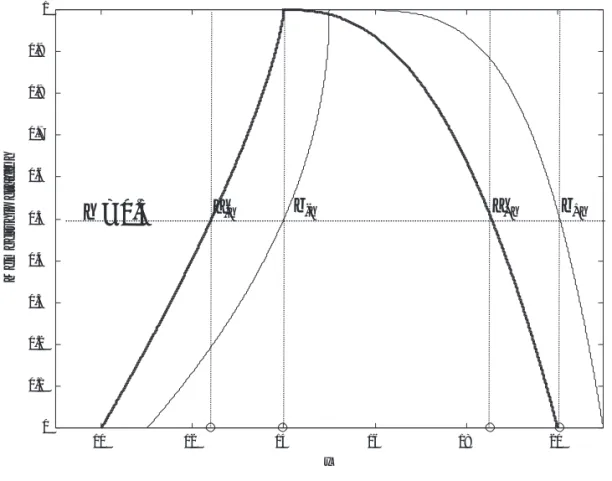
The fact that a value of r = 30 is outside the data range is
Fig. 7. Observed (squares) and estimated (lines) tree growth of Pinus pinea L. at Vidauban. The estimates are obtained from a classical linear regression (LR) model (lower graph) and from a fuzzy LR model with h = 0.5 and h = 0.75 (upper graph). The observations are represented by squares. LR estimates are presented with 95% confidence intervals.not really a problem, as a value this extreme, such as a value
with a null error bar, is not really observable.
To use eq. 11 in the calculations, select any level h in [0,
1] and rewrite eq. 11 in interval form (
α
> r = 30) taking
ac-count of eq. 7:
[12]
z h
a
h
a
h
r
z h
a Pa a Pa − +=
−
−
+
−
−
−
=
( )
(
)
[
(
)
](
)
( )
0 01
1 11
1 0 1 1δ
δ
α
a
0 a01
h
q aa
1 a11
h
q ar
1 0 1 1+
η
(
−
)
+
[
+
η
(
−
)
](
α
−
)
Note that some confusion may remain between the
credibil-ity level h applied to solve the LP problem (i.e., the h value
for which we compute the fuzzy numbers ~
a
0and ~
a
1) and the
level h used to represent them in interval terms as written in
eq. 12. It will be discussed below.
The minimization of the linear objective function subject
to linear constraints constitutes a so-called LP problem. In
this LP problem, the profile of the membership function of
the coefficients and dependent variable is to be selected. The
~
y
thave already been taken as triangular fuzzy numbers. We
make the same choice for ~
a
0. To take account of the fact that
low values of
α
are much more constraining than high
val-ues, we choose an asymmetric membership function for ~
a
1defined by the equation with p = 0.2 (with a small area) and
q = 5 (with a larger area).
The grade h is specified to solve the LP problem, which
then yields equations for z
–and z
+that are functions of
any h, and then h is chosen as a particular value to provide
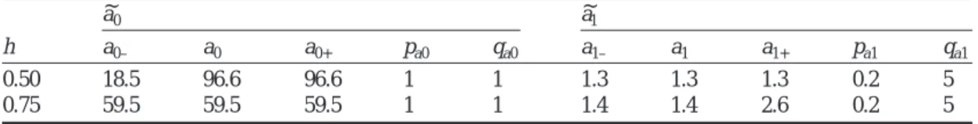
the results. We give them in Table 4 for two levels of h. At
h = 0.50, the LP problem yields a triangular fuzzy number
~
a
0and a crisp ~
a
1. At h = 0.75, the LP problem gives a crisp
~
a
0and ~
a
1as an LRFN. From eq. 12 these results can be
written as follows:
[13]
h
z
h
z
=
⇒
=
−
− +
−
=
+
−
− +0 5
966
7811
13
30
966
13
30
.
.
. (
)
. (
)
.
. (
)
α
α
[14]
h
z
z
h
=
⇒
=
+
−
=
+
+
−
− +0 75
595
14
30
595
14
12 1
15.
.
. (
)
.
[ .
. (
) ](
α
α −
30)
The predictions obtained by these equations are displayed in
Fig. 7, which calls for the following comments.
(1) As pointed out before, the credibility level from which
the LP problem has been solved should not be confused
with the level h used to sketch the results. Here we
solved the LP problem for h = 0.5 and h = 0.75 while
we drafted the figure with h = 0.5. (This value must be
lower or equal to the value of h for which the
mini-mization has been done.)
(2) The LP problem for h = 0.5 returns two parallel straight
lines meaning that the uncertainty does not depend upon
the ratio
α
. Of course such a conclusion stems from the
fact that the coefficient ~
a
1has been found crisp, but
there is no physical argument to support this result.
(3) The LP problem for h = 0.75 envelops the input points
between two divergent straight lines indicating that the
uncertainty increases with the distance from the
refer-ence point. This result is in accordance with our
inter-pretation of the problem: low values of
α
limit
tree-growth, while other factors are limiting for high
values of
α
; this increases the uncertainty of the
predic-tion using only
α
.
(4) The classical linear regression (LR) provides predictions
closer to the lower limit of those provided by the fuzzy
regression, but the narrowest error bars are obtained for
values close to the mean climate, even if a mean
α
is
certainly less limiting for the growth than a low
α
. The
consequence of the asymmetry of the fuzzy number (G
1,
G
2, G
3) constructed to take into account the limiting
factor principle is certainly closer to the biology of the
problem.
Comparison with classical approach
The fuzzy approach gives results comparable with those
obtained using a classical linear regression. Furthermore, the
fuzzy approach selects the same variable as limiting factor
as the classical linear regression. However, ordinary
classi-cal regression does not give any information about which
values of the environmental parameters are the most
limit-ing. The classical response function just tells us that, on
av-erage, a low
α
= AET/PET limits the growth and a high
α
favours the growth.
Furthermore, classical response functions have proved to
be particularly efficient for trees growing in such drastic
conditions that the limiting factor is unique throughout the
year and from year to year. Such situations induce a high
variability in tree-ring width and define sensitive trees in
op-position to complacent trees characterized by ring-width
se-ries without any variability. In fact, this situation can also be
contrasted to situations were growth is limited by the
fluctu-ations of multiple limiting factors whose combination varies
during the year and from year to year. Such situations induce
a high variability of ring width and correspond also to
sensi-tive trees. In this situation, the classical response function
provides poor information because of the nonstationarity of
the combination of potential explicative variables. We can
assume that the use of fuzzy regression will provide
infor-mation about the threshold about which a parameter is
involved in the control of tree growth. The fuzzy approach
enables one to test separately the different variables after an
~a0 ~a1
h a0– a0 a0+ pa0 qa0 a1– a1 a1+ pa1 qa1
0.50 18.5 96.6 96.6 1 1 1.3 1.3 1.3 0.2 5
0.75 59.5 59.5 59.5 1 1 1.4 1.4 2.6 0.2 5
Note: The fuzzy parameters are LRFN with fixed left right membership functions. The LP problem is solved for two
levels of h.
Table 4. Fuzzy linear regression between the crisp input variableα; AET/PET and the fuzzy (TFN) output variable ~y; tree growth.
a priori selection of these variables on the basis of the
un-derstanding of the tree environment (climate, elevation,
sub-stratum). This would be a first step in the construction of a
type of “growth simulator” adapted to the different
environ-ments of a given species.
Specific advantages of fuzzy linear regression
The first remarkable point in the results given by the
fuzzy response function is that the concept of limiting factor
seems to be taken into account much more strongly. The
in-terval of credibility given by the fuzzy regression suggests
that better growth predictability is obtained for high water
stress (i.e., low values of
α
), which is typical of
Mediterra-nean climate. This information was included into the model
a priori by selecting the reference value of
α
= 30, but it has
been confirmed a posteriori by the results (see eq. 6). For
higher values (>65%),
α
loses the status of limiting factor
and the error intervals become larger. By comparison, the
classical regression seems to give a better precision for
val-ues close to the mean climate, which is far from the biology
of the problem.
Next, fuzzy regression can be also a method to test
differ-ent hypotheses on several potdiffer-ential predictors when any
fur-ther experimental approach is quite impossible, as it is for
testing response models in risk analysis at very low doses
(Bardossy et al. 1993) or for trees in their natural
environ-ment. Several tests can be envisaged.
(1) For a unique population, when different climatic
vari-ables are correlated with tree growth (as shown by a
preliminary linear regression), these variables can be
in-troduced in turn as unique predictors into a fuzzy model
to identify which values are the most limiting; this can
be done by changing the reference value and the
mem-bership function profile.
(2) The same potential explanatory variable
α
could be
tested for different populations selected by modifying
the threshold for which this parameter remains limiting.
Such a procedure could be implemented for example on
the basis of edaphic characteristics or elevation in the
same climatic area.
Weaknesses of fuzzy linear regression
The practitioners of fuzzy linear regression claim that it is
a robust form of regression. However, it has been shown
(Redden and Woodall 1996) that (i) fuzzy linear regression
is sensitive to outliers; (ii) the fuzzy linear algorithm cannot
take all of the the available information into account
(redun-dant constraints in the LP problem); and (iii) the algorithm
can produce crisp coefficients. (A crisp coefficient occurs
when the width of the fuzzy regression coefficient is 0.)
The first two remarks are not specific to fuzzy linear
re-gression. Ordinary least squares and orthogonal least squares
are all known to be sensitive to outliers and influential
points. That is why we explicitly removed any outlier. With
regard to the available information, the constrained
optimi-zation involves inequalities that can be redundant. In any
case, the relevance of constrained optimization in decision
making is not in question. With regard to crisp coefficients,
the fuzzy linear algorithm really can produce crisp
coeffi-cients. The reason is that we seek fuzzy coefficients that
possess minimum fuzziness. All the same, as soon as at least
one coefficient is not crisp, the response is clearly fuzzy.
Another issue is the interpretation of the predicted fuzzy
numbers. How does a practitioner measure the relevance of
its fuzzy response function? How does a practitioner decide
whether or not to add an explanatory variable in the fuzzy
linear regression? This issue is not as yet resolved.
Nevertheless, we claim that the environmentalist has three
reasons to consider fuzzy linear regression. The first results
from the realization that it is often not realistic to assume
that a crisp function represents the relationship between the
given variables. The second comes from the nature of data,
which in environmental sciences are inherently fuzzy. The
third reason is that the fuzzy concepts are very intuitive
making the practitioner more responsible over its own
back-ground and field of study.
Often in environmental sciences we are confronted with
uncertain facts and scarce and imprecise data. For instance,
some environmental experiments cannot be repeated a lot of
time because they are very expensive and (or) destructive. In
that case the response Y to the control X is often doubtful.
As an alternative to classical regression, fuzzy linear
regres-sion was introduced (Tanaka et al. 1982).
A fuzzy regression aims to envelop the limited
observa-tions for the case when the control X is crisp and the
vague-ness of the response Y is described in terms of fuzzy
numbers. This technique makes it possible to take into
ac-count not only the uncertainty in the response but also that
stemming from the selected relationship. In addition,
devia-tions between the observed values and the estimated values
(i.e., the errors) are fully taken into account by the fuzziness
of the coefficients. The fuzzy response function thus appears
to be an approach between the mechanistic and the statistical
descriptive approaches.
This study was made possible thanks to support provided
by the cooperation program between the Commissariat
général aux relations internationales de la Communauté
française de Belgique, the Fond national de la recherche
scientifique, and the Centre national de la recherche
scientifique. We are grateful to Professor Lucien Duckstein,
University of Arizona, and the École nationale du génie
ru-ral, des eaux et des forêts, Paris, France, who corrected and
commented on the manuscript.
Badeau, V., Dupouey, J.L., Becker, M., and Picard, J.F. 1995. Long-term growth trends of Fagus sylvatica L. in northeastern France. A comparison between high and low density stands. Acta Oecol. 16: 571–583.
Bardossy, A., Bogardi, I., and Duckstein, L. 1990. Fuzzy regres-sion in hydrology. Water Resour. Res. 26: 1497–1508. Bardossy, A., Duckstein, L., and Bogardi, I. 1993. Fuzzy
non-linear regression analysis of dose response relationship. Eur. J. Oper. Res. 66: 36–51.
Berger, J.O. 1985. Statistical decision theory and Bayesian analy-sis. Springer-Verlag, New York.
Bernier, J. 1987. Elements of Bayesian analysis of uncertainty in hydrological reliability and risk models. In Engineering reliabil-ity and risk in water resources. Edited by L. Duckstein and E. Plate. Martinus Nijhoff, Boston, Mass. pp. 405–421.
Bert, G.D. 1992. Influence du climat, des facteurs stationnels et de la pollution sur la croissance et l’état sanitaire du sapin pectiné (Abies alba) dans le jura. Ph.D. thesis, Université de Nancy, Nancy, France.
Boreux, J.J., Pesti, G., Nicolas, J., and Duckstein, L. 1997. Age model estimation in paleoclimatic research: fuzzy regression and radiocarbon uncertainties. Palaeogeogr. Palaeoclim. Palaeoecol. 128: 29–37.
Burman, R., and Pochop, L. 1994. Evaporation, evapotranspiration and climatic data. Dev. Atmos. Sci. No. 22.
Caselton, W.F., and Luo, W. 1994. Inference and decision under near ignorance conditions. Engineering risk in natural resources management with special references to hydrosystems under changes of physical or climatic environment. Edited by L. Duckstein and E. Parent. Kluwer Academic Publishers, Dordrecht, the Netherlands. pp. 291–303.
Chu, C., and Marron, J. 1991. Choosing a kernel regression esti-mator (with discussion). Stat. Sci. 6: 404–436.
Cropper, J.P. 1982. Comment on response functions. In Climate from tree-rings. Edited by M.K. Hughes, P.M. Kelly, J.R. Pilcher, V.C. LaMarche Jr. Cambridge University Press, Cam-bridge, U.K. pp. 38–45.
Douglass, A.E. 1936. Climatic cycles and tree-growth. Vol. 3. A study of cycle. Carnagie Inst. Wash. Publ. No. 289.
Dubois, D., and Prade, H. 1980. Fuzzy sets and system theory and applications. Academic Press, San Diego, Calif.
Efron, B. 1979. Bootstrap methods: another look at the jackknife. Ann. Stat. 7: 1–26.
Efron, B. 1983. Estimating the error rate of a prediction rule: im-provement on cross-validation. J. Am. Stat. Assoc. 78: 316–331. Emberger, L. 1930. La végétation de la région méditerranéenne. Essai d’une classification des groupements végétaux. Rev. Gen. Bot. 42: 641–662 and 705–721.
Fan, J., and Gijbels, I. 1982. Local polynomial modelling and its applications. Chapman & Hall, London, U.K.
Federer, C.A. 1982. Transpirational supply and demand: plant, soil, and atmospheric effects evaluated by simulation. Water Resour. Res. 18: 355–362.
Fritts, H.C. 1976. Tree-rings and climate. Academic Press, Lon-don, U.K.
Fritts, H.C. 1982. The climate growth response. In Climate from tree-rings. Edited by M.K. Hughes, P.M. Kelly, J.R. Pilcher, V.C. LaMarche Jr. Cambridge University Press, Cambridge, U.K. pp. 38–45.
Fritts, H.C., Blasing, T.J., Hayden, B.P. and Kutzbach, J.E. 1971. Multivariate techniques for specifying tree-growth and climate relationships and for reconstructing anomalies in paleoclimate. J. Appl. Meteorol. 10: 845–864.
Gadbin-Henry, C. 1994. Études dendroécologiques de Pinus pinea L. Aspects méthodologiques. Ph.D. thesis, Université d’Aix-Marseille III, Aix-en-Provence, France.
Guiot, J. 1989. Method of calibration and comparison of methods. In Methods of dendrochronology. Edited by E.R Cook. and L.A Kairiukstis. Kluwer Academic Publishers and International In-stitute for Applied Systems Analysis, Dordrecht, the Nether-lands. pp. 165–178 and 185–193.
Guiot, J., and Tessier, L. 1997. Detection of pollution signals in tree-ring series using AR processes and neural networks. In Ap-plications of time-series analysis in astronomy and meteorology. Edited by T.S. Rao, M.B. Priestley, and O. Lessi. Chapman & Hall, London, U.K. pp. 413–426.
Guiot, J., Berger, A.L., and Munaut, A.V. 1982a. Response func-tions. In Climate from tree-rings. Edited by M.K. Hughes, P.M. Kelly, J.R. Pilcher, V.C. LaMarche Jr. Cambridge University Press, Cambridge, U.K. pp. 38–45.
Guiot, J., Berger, A.L. Munaut, A.V., and Till, C. 1982b. Some new mathematical procedures in dendroclimatology with exam-ples for Switzerland and Morocco. Tree-Ring Bull. 42: 33–48. Harrison, S.P., Prentice, I.C., and Guiot, J. 1993. Climatic controls
of Holocene lake-level changes in Europe. Clim. Dyn. 8: 189–200.
Hastie, T., and Loader, C. 1993. Local regression: automatical ker-nel carpentry (with discussion). Stat. Sci. 8: 120–143.
Heshmaty, B., and Kandel, A. 1985. Fuzzy linear regression and its applications to forecasting in uncertain environment. Fuzzy Sets Syst. 15: 159–191.
Jarvis, P.G., and MacNaughton, K.G. 1986: Stomatal control of transpiration: scaling up from leaf to region. Adv. Ecol. Res. No. 15. pp. 1–49.
Kaufmann, A., and Gupta, M.M. 1991. Introduction to fuzzy arith-metic: theory and applications. Van Nostrand Reinhold, New York.
Lebourgeois, F. 1995. Étude dendroécologique et écophysiologique du Pin laricio de Corse (Pinus nigra A. ssp. laricio) en région pays de Loire. Ph.D. thesis, Université de Paris-Sud, Orsay, Paris, France.
Neter, J., Wasserman, W., and Kutner, M.H. 1989. Applied linear regression models. 2nd ed. Irwin, Homewood, Ill.
Prentice, I.C., Cramer, W., Harrison, S.P., Leemans, R., and Monserud, R.A. 1992. A global biome model based on plant physiology and dominance, soil properties and climate. J. Biogeogr. 19: 117–134.
Prentice, I.C., Sykes, M.T., and Cramer, W. 1993. A simulation model for the transient effects of climate change on forest land-scapes. Ecol. Modell. 65: 51–71.
Redden, D.T., and Woodall, H. 1996. Further examination of fuzzy linear regression. Fuzzy Sets Syst. 79: 203–211.
Schweingruber, F.H., Kairiukstis, L., and Shiyatov, S. 1990. Sam-ple selection. In Methods of dendrochronology. Edited by E.R Cook and L.A Kairiukstis. Kluwer Academic Publishers and IIASA, Dordrecht, the Netherlands. pp. 23–96.
Shashkin, A.V., and Fritts, H.C. 1995. A model that simulates cambial activity and ring structure in conifers. In Tree rings, from the past to the future. Edited by S. Ohta and M.K. Hughes. Forestry and Forest Products Research Institute, Tsukuba, Japan. pp. 24–30.
Tanaka, H., Uejima, S., and Asai, K. 1982. Linear regression anal-ysis with fuzzy model. IEEE Trans. Syst. Man Cybern. 12: 903–907.
Viertl, R. 1997. Non-precise information in Bayesian inference. In Statistical and Bayesian methods in hydrological sciences. Edited by E. Parent and B. Bobie. UNESCO Press, Paris. pp. 465–478.
Zadeh, L.A. 1965. Fuzzy sets. Inf. Control, 8: 338–353.
Zadeh, L.A. 1973. Outline of a new approach to the analysis of complex systems and decision processes. IEEE Trans. Syst. Man. Cybern. 3: 28–44.