Classification for ternary flash point mixtures diagrams regarding miscible flammable compounds

HAL Id: hal-01831762

https://hal.archives-ouvertes.fr/hal-01831762

Submitted on 6 Jul 2018

HAL is a multi-disciplinary open access

archive for the deposit and dissemination of

sci-entific research documents, whether they are

pub-lished or not. The documents may come from

teaching and research institutions in France or

abroad, or from public or private research centers.

L’archive ouverte pluridisciplinaire HAL, est

destinée au dépôt et à la diffusion de documents

scientifiques de niveau recherche, publiés ou non,

émanant des établissements d’enseignement et de

recherche français ou étrangers, des laboratoires

publics ou privés.

Classification for ternary flash point mixtures diagrams

regarding miscible flammable compounds

Sergio da Cunha, Vincent Gerbaud, Nataliya Shcherbakova, Horng-Jang Liaw

To cite this version:

Sergio da Cunha, Vincent Gerbaud, Nataliya Shcherbakova, Horng-Jang Liaw. Classification for

ternary flash point mixtures diagrams regarding miscible flammable compounds. Fluid Phase

Equi-libria, Elsevier, 2018, 466, pp.110-123. �10.1016/j.fluid.2018.03.010�. �hal-01831762�

O

pen

A

rchive

T

OULOUSE

A

rchive

O

uverte (

OATAO

)

OATAO is an open access repository that collects the work of Toulouse researchers and

makes it freely available over the web where possible.

This is an author-deposited version published in :

http://oatao.univ-toulouse.fr/

Eprints ID : 20323

To link to this article : DOI:

10.1016/j.fluid.2018.03.010

URL :

https://doi.org/10.1016/j.fluid.2018.03.010

To cite this version :

Da Cunha, Sergio and Gerbaud, Vincent and

Shcherbakova, Nataliya and Liaw, Horng-Jang Classification for

ternary flash point mixtures diagrams regarding miscible flammable

compounds. (2018) Fluid Phase Equilibria, 466. 110-123. ISSN

0378-3812

Any correspondence concerning this service should be sent to the repository

administrator:

staff-oatao@listes-diff.inp-toulouse.fr

Classification for ternary flash point mixtures diagrams regarding

miscible flammable compounds

Sergio da Cunha

, Vincent Gerbaud

, Nataliya Shcherbakova

, Horng-Jang Liaw

a_{Universit!e de Toulouse, INP, UPS, LGC (Laboratoire de G!enie Chimique), 4 all!ee Emile Monso, F-31432 Toulouse Cedex 04, France} b_{Department of Safety, Health, and Environmental Engineering, National Kaohsiung First University of Science and Technology, Taiwan, ROC}

Keywords:

Flash point

Miscible flammable compound Nonequilibrium thermodynamics Classification

Ternary diagrams

a b s t r a c t

Flash point is a major indicator on the study of fire and explosion hazards of liquid mixtures. Mixtures presenting a minimum flash point behavior are particularly dangerous. It has been shown before that minimum/maximum flash point mixtures could be related with azeotropic behavior under some con-ditions. Since the 70's a classification of ternary azeotropic mixtures has been developed based on the topological properties of residue curve maps arising from the simple evaporation equilibrium model. In this paper we show that such a general classification also exists for flash point diagram of miscible flammable compound ternary mixtures and that it could help anticipate fire and explosion hazard in ternary mixtures. The demonstration is based on the construction of an auxiliary theoretical system under equilibrium equivalent to a non-equilibrium flash point system.

1. Introduction

The study of flash point temperature of mixtures plays an important role for the safety in the chemical industry. Several ac-cidents due to explosions [1e3] highlight the importance of knowing the flash point temperature in pure compounds and mixtures.

Since the flash point data available for mixtures is quite scarce, several different methods have been proposed to compute the flash point of different types of mixtures. The first method based on the assumption of Vapor-Liquid Equilibrium (VLE)

m

i¼

m

air) was developed for flammable miscible mixtures [4] and then extended for miscible mixtures with flammable and non-flammable compounds [5,6]. Liaw et al. [7] showed that miscible mixtures of flammable compounds satisfy the following equation:

Xc i¼1 xi

g

Here c is the number of flammable components in the mixture, and for each liquid phase component i ¼ 1;…

;c xi represents the

corresponding mole fraction,

g

Psat

i denotes the saturation pressure and Pisat;fp

denotes the saturation pressure at the flash point temperature. T is the flash point tem-perature of the system and x ¼ ðx1; x2; …;xc$1Þ is the composition vector.

Eq. (1)is derived by assuming that each component i in the vapor-air mixture (excluding the air) is in equilibrium with the liquid mixture and that the vapor-phase behaves like an ideal gas because of the flash point being measured under atmospheric pressure. Under these assumptions, the following equation holds true:

yi¼

xi

g

Psyst (2)

Model described by eq. (1) can also be extended to partially miscible mixtures [8e11]. The models referred above are based on two main assumptions: xair¼ 0 and equality of chemical potentials

for the remaining components. The last assumption suggests to generalize the classical equilibrium approach used to describe the distillation curves and boiling temperature surfaces in the theory of vaporeliquid equilibrium [12]. The similarity between both flash point and boiling point description has been highlighted in previ-ous works [5,13]. We have recently addressed a relation between the occurrence of azeotropic behavior and minimum/maximum

*Corresponding author.

E-mail address:vincent.gerbaud@ensiacet.fr(V. Gerbaud).

flash point in binary mixtures and showed it to be dependent on the ratio DTfp

DTb of pure component flash point and boiling point

temperature differences [14].

In the VLE equilibrium theory, the topology of the boiling point temperature surfaces is intrinsically connected to the structure of the VLE diagrams describing the residue curves maps. The most compact and consistent classification of ternary VLE diagrams was first proposed by Gurikov in 1958 and then improved by Serafimov in 1970 [12], who established 26 classical feasible structures for these diagrams under certain conditions on the number and type of possible azeotropes. This classification have been derived from the Poincare's topological theory of dynamical systems applied to the residue curves differential equations arising in the open evapora-tion equilibrium model [12,15].

The aim of the present article is to propose a classification for the flash point temperature surfaces of ternary mixtures of miscible flammable compounds. Such a classification may simplify the detection of ternary extremum flash point behaviors, which can increase the hazards of fire and explosion in the case of a minimum flash point. The new classification is inspired by Serafimov's clas-sification of ternary azeotropic mixtures and its direct transposition for boiling temperature isotherms diagrams describing the open evaporation under thermodynamic equilibrium conditions at con-stant pressure. However, the boiling temperature results cannot be directly extended to the flash point closedecup systems, since the presence of air does not allow the whole system (biphasic LV mixture þ air) to be in thermodynamic equilibrium, as we shall explain later. Hence, the key idea of the theoretical part of this paper is the proof of a formal equivalence of a closed-cup system with an auxiliary VLE system with properly selected components. This equivalence allows the extension of the VLE Serafimov's clas-sification to the flash point closed-cup systems.

The paper is organized as follows. In Section2we recall the main facts about simple distillation of homogeneous mixtures under thermodynamic equilibrium condition. In particular, we recall the properties of their residue curve maps in connection with the structure of the associated boiling temperature surfaces, and

the main principles underlying the Serafimov's classification of ternary VLE diagrams. In Section3we consider flash point closed-cup ternary systems and propose an approach leading to a classi-fication of the ternary flash point closed-cup systems. In Section4

we discuss several experimental and simulation results through the prism of the theoretical part of this work.

2. Distillation under thermodynamic equilibrium: summary

2.1. Thermodynamic equilibrium for closed bi-phasic systems

Consider a closed c-component bi-phasic system. Let Tl ðvÞ_and

PlðvÞ_{denote the temperature and the pressure of each phase, the}

superscripts l and v referring to the liquid and to the vapor phase respectively. By xi and yi we denote the mole fractions of the

component i in the liquid and in the vapor phases. An example of such a system for c ¼ 3 is represented inFig. 1.

The thermodynamic equilibrium is reached when the following set of conditions is satisfied:

Tl_{¼ T}v ; P l_{¼ P}v ;

m

m

Here

m

According to Lewis [16] the fugacity fiof the i-th component is

defined as follows:

m

m

In the above equation,

m

i and fi0denote the chemical potential

and the fugacity at a given reference state. It can be proven [16,17] that the equality of the chemical potentials of each component in two phases at the thermodynamic equilibrium is equivalent to the equality of their corresponding fugacities:

fl i ¼ f

v

i; i ¼ 1;…

;c (5)

2.2. Simple distillation and the residue curve maps

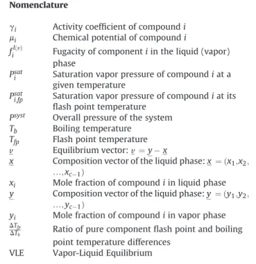
Distillation is a process of separation of liquid mixtures based on the differences among the relative volatility of their components. Nomenclature

g

m

f_ilðvÞ Fugacity of component i in the liquid (vapor) phase

Psat

i Saturation vapor pressure of compound i at a

given temperature

Psat i;fp

Saturation vapor pressure of compound i at its flash point temperature

Psyst _{Overall pressure of the system}

T_b Boiling temperature

Tfp Flash point temperature

v Equilibrium vector: v ¼ y $ x

x Composition vector of the liquid phase: x ¼ ðx1;x2; …

;xc$1Þ

xi Mole fraction of compound i in liquid phase

y Composition vector of the liquid phase: y ¼ ðy1;y2; …

;yc$1Þ

yi Mole fraction of compound i in vapor phase

DTfp

DTb Ratio of pure component flash point and boiling

point temperature differences VLE Vapor-Liquid Equilibrium

The most volatile components concentrate in vapor phase, enriching the remaining liquid phase with the less volatile com-ponents. The simple distillation (or open evaporation) is the simplest type of distillation, in which the liquid is boiling in a still at constant pressure and the created vapor is continuously evacuated from the system. The system as a whole is kept at thermodynamic equilibrium between the liquid and the vapor phases, so that re-lations (3) are satisfied at any time [12]. Models of simple distilla-tion give rise to a set of differential equadistilla-tions which can be analyzed with concepts from the field of topology in mathematics to establish the concise and complete Serafimov's classification of boiling point temperature diagrams. We now recall the main steps leading to such a classification.

According to the phase rule [17], the total number of degrees of freedom in an c-component bi-phasic liquid-vapor heterogeneous system is equal to c. SincePc_i¼1xi ¼ 1, by assuming that the process

is isobaric (P ¼ const), we can choose the first c $ 1 liquid mole fractions (independent variables) and the temperature T (depen-dent variable) to describe the whole state space of the system. Applying mass balances, the evolution of the liquid composition in such process can be described by the set of differential equations [18]:

dxi

d

x

where

x

liquid phase:

x

!

. The right-hand sides of the residue curve differential eq.(6)form the equilibrium vector field v ¼ ðx1$

y1;…

;xc$1$ yc$1Þ in the c $ 1-dimensional composition space of

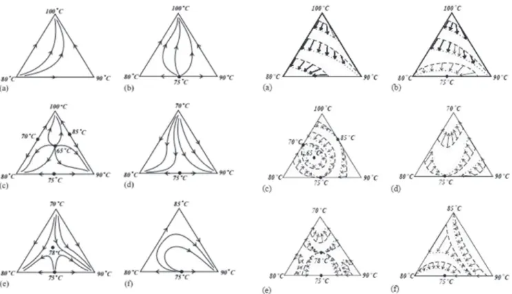
the system. Its integral curves, solutions to eq.(6), are called the residue curves. The set of such curves forms a residue curves map (RCM) of a given mixture. In the left part ofFig. 2we show several examples of RCMs in case of ternary systems.

The topological structure of RCMs is intrinsically related to the properties of the boiling temperature of the mixture. Indeed, in order to compute the residue curves by solving eq.(6), one should complete it with the VLE condition for isobaric processes:

Xc

i¼1

yiðx;TÞ ¼ 1 (7)

Here the functions yiðx;TÞ are to be defined by an appropriate

thermodynamic model. Eq. (7) defines a hyper-surface in the

c-dimensional state space fðx; TÞg, called the boiling temperature surface. Even though eq.(7)defines this surface only implicitly, it can in theory be solved with respect to the temperature. So, the boiling temperature surface can be represented in the form T ¼

TbðxÞ, i.e., as a graph of the boiling temperature function

TbðxÞ corresponding to the given composition x. The right part of Fig. 2shows the isotherms, i.e. the level sets of the function T_bfor the ternary mixtures shown on the left of Fig. 2. The arrows describing the inverse evolution of the level sets correspond to the inverse of the equilibrium vector field. The exact relation between the equilibrium vector field v and the boiling temperature follows from a more general argument.

Indeed, in alternative to eq.(7), the boiling temperature along the residue curves can be recovered from the generalized Van der Waals e Storonkin equation [19], which follows directly from the second law of thermodynamics. It provides another theoretical way to define the thermodynamic equilibrium condition in the differ-ential form:

Fig. 2. eResidue curve maps of ternary mixtures (left) and their respective boiling temperature isotherms (right), extracted fromFig. 4andFig. 6in Kiva et al. (2003) [12]. Copyright 2003 Elsevier.

D

c$1 i;j¼1

v2_gl

v_xiv_xjðxi$ yiÞdxj¼ 0 (8)

Here gl_{denotes the Gibbs free energy of the liquid phase and the}

function

D

D

In the above expression slðvÞ_{and s}lðvÞ

i denote the overall and the

partial molar entropies of the liquid (vapor) phases. As it was recently shown in Ref. [20], eq. (8)implies that the equilibrium vector v restricted to the boiling temperature surface is equal to the generalized gradient of the boiling temperature function Tb:

vðxÞ ¼defvðx;T_bðxÞÞ ¼

D

D2xgl

&$1

V_TbðxÞ¼defVG_{TbðxÞ (9)}

where the gradient VGis defined with respect to the Riemannian metric associated to the Hessian D2

xglof the Gibbs free energy gl

normalized by the entropy term

D

one-to-one correspondence between the topology of the boiling temperature surface and the underlying RCM.

2.3. Singularities of the RCMs

The main topological characteristics of a RCM is the structure of its singular points defined by the set of points where the equilib-rium vector field v vanishes and hence

xi¼ yi; i ¼ 1;…

;c (10)

These points are stationary points of the dynamical system described by eq.(6). Physically, singular points represent the pure states of the components or the azeotropic compositions and are thus of practical importance. Under generic conditions, the singular points of the RCM can only be of node (stable or unstable) or saddle types. Before its formal demonstration [15,19], this fact was established experimentally [12,21]. In Fig. 3 we show the local behavior of the residue curves in the vicinity of the singular points in the ternary case.

SN, UN and S inFig. 3refer respectively to stable node, unstable node and saddle point. The only possible types of the RCMs singular points are imposed by the gradient type of the dynamical system in eq.(6)[20]. Moreover, according to eq.(9), the singular points of a RCM are the critical points of the associated boiling temperature

function Tb. More precisely, in the ternary case [15,22], the stable/

instable nodes correspond to the minimum/maximum points of the boiling temperature surface, and the saddles correspond to the saddle points on this surface. Such a duality between the types of singularities of the RCM and the critical points of the associated boiling temperature function can be easily seen by comparing the two sides ofFig. 2. According to the shape of the isotherms in the vicinity of a critical point, one can distinguish the elliptic-type points corresponding to the maxima/minima of the boiling tem-perature (i.e., to the nodes of the RCM), and the hyperbolic-type points corresponding to saddles.

2.4. Serafimov's classification of ternary VLE diagrams

The classification of the ternary VLE diagrams is based on following nomenclature of the singular points of ternary RCMs:

N1 number of pure states of node (stable or unstable) type

(Fig. 3a);

N2 number of binary azeotropes of node (stable or unstable)

type (Fig. 3b);

N3number of ternary azeotropes of node (stable or unstable)

type (Fig. 3c);

S1number of pure states of saddle type (Fig. 3d);

S2number of binary azeotropes of saddle type (Fig. 3e);

S3number of ternary azeotropes of saddle type (Fig. 4f)

The Poincare - Hopf Index Theorem (see in Milnor (1965) [23] for more details) implies a strict rule relating the total number of singularities of a dynamical system with their type. In the case of a ternary VLE system, it has the following form [15,24]:

2N3þ N2þ N1¼ 2S3þ S2þ 2 (11)

Serafimov's classification of ternary RCM diagrams is based on this rule, completed by the following assumptions:

(i) the diagram contains at most one binary azeotrope for each binary pair of components (N2þ S2* 3);

(ii) the diagram contains at most one ternary azeotrope (N3þ S3* 1);

(iii) only generic (saddles and nodes) azeotropes are taken into account.

Assumptions (i) e (iii) hold, except for a few rare cases with multiple binary azeotropes and ternary azeotropes [25]. Using eq.

(11)constraint with assumptions (i) e (iii), Gurikov [24] proposed

the first classification for ternary VLE diagrams, which was then improved by Serafimov in 1970's [12].Fig. 4shows the 26 standard Serafimov's classes which describe all possible topological struc-tures of ternary RCM diagrams verifying assumptions (i) - (iii).

In this figure, the symbols (+) and (◦) refer to stable (unstable) and unstable (stable) nodes, and V to a saddle point. Note that the interchange of stable and unstable nodes simply reverses the di-rection of the residue curves: the residue curves converge to stable nodes, diverge from unstable nodes and have hyperbolic behavior near the saddle points. The above classification uses the so-called

b.t-z notation, where b refers to the number of binary stationary

points, t refers to the number of ternary stationary points and z

allows to distinguish diagrams with the same b and t numbers but with different residues curves shapes [12].

In view of the duality between the location and the type of singular points of the RCM and the critical points of the corre-sponding boiling temperature, it is possible to classify the feasible topological classes of the VLE systems according to the type of the boiling temperature critical points and the shape of the isotherm curves instead of the residue curves, as it was proposed in Ser-afimov et al. (2012) [27]. In the next section we extend this approach to theflash point temperature surfaces of flammable systems.

3. Classification of the flash point temperature critical points There exist various standard test methods for flash point mea-surement. Heat rate is one of the differences in the values of experimental parameters between these test methods. For example, heat rate-1 is 1,_{C/min, 5e6},_{C/min, and 1.3},_{C/min for}

ASTM D56, ASTM D93A and ASTM D93B, respectively. The degree of equilibrium between liquid phase and gas phase is affected by the heat rate during the flash point test, with low heat rate, long equilibrium time, more approaching to equilibrium. It seems the suitability of this study may depend on the standard test methods. However, our previous study indicated that the difference in the measured values of flash point for 1% (molar fraction) of ethanol mixed with 99% of tetradecane is small, with the measured value being 39.5,_{C and 41.3},_{C when based on ASTM D56 and ASTM 93B,}

respectively [28]. In addition, Eq.(1)is applicable to the mixtures when based on the flash point values of individual components, irrespective of the data are obtained by the standard test method ASTM D56, ASTM D93A, ASTM D1310-86 or ASTM D3971 [5e7,13,29e31], and it is more reliable than other models [31e33]. It seems that the vapor liquid equilibrium assumption for the mixtures' components except for air, assumption in deriving Eq.(1), is applicable in flash point prediction.

In this section we focus on the closed-cup flash point of ternary mixtures. All the experimental data used in this study to validate the proposed theory were obtained according to ASTM D56, with low heat rate. On one hand we remark that the VLE theory argu-ments cannot be applied straightforwardly to this flash point sys-tem since not all the components are at thermodynamic equilibrium for the latter. On the other hand, the available experi-mental data and the results of numerical simulations of ternary flammable mixtures suggest that flash point and boiling point surfaces have similar topologies, as we prove below. In order to validate this conjecture, first we have to re-consider the thermo-dynamic properties of the flammable mixtures. Below we focus on ternary mixtures, but the same arguments remain valid for any number of components.

3.1. A closed-cup flash point system and the thermodynamic equilibrium

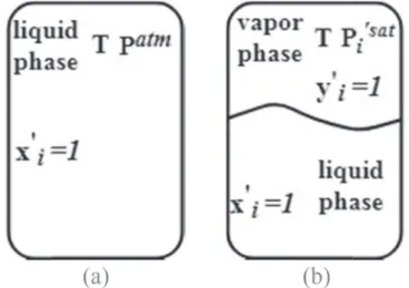
Let us look in detail at the closed-cup flash point system con-taining components 1, 2 and 3 in both liquid and vapor phases, and component 4, air, being presented only in the vapor phase.Fig. 5a represents the closed-cupflash point test, described by ASTM D 56 [34]. The pressure for the flash point measurement is kept constant and equal to the atmospheric pressure. A spark is produced for a set of temperatures, and the lowest temperature for which the spark generates a flame is defined as the flash point temperature T for that mixture at a given composition and pressure. It is assumed that the described system, named as system S, satisfies the following assumptions:

(a) the vapor phase has an ideal behavior;

(b) each component i in the vapor-air mixture (excluding the air) is in equilibrium with the liquid mixture.

Under these assumptions, eqs.(1) and (2)are valid. However, system S inFig. 5a is not strictly at equilibrium, since the air is assumed to be present only in the vapor phase. For this reason, the chemical potentials of air in the two phases are different, and the last of eq.(3)is not satisfied.

Now let us consider another system represented inFig. 5b and referred below as the system S’. Hereafter the “0_{” symbol is used to}

mark its parameters.

The system S0_{is composed of three compounds 1}0_{, 2}0_{and 3’. We}

assume that these compounds have the same interactions in the liquid phase as the compounds 1, 2 and 3 of the system S, i.e., for a given temperature Tand liquid composition x1;x2;x3, the activity coefficients

g

g

0

iare the same. In contrast, the thermodynamic

characteristics of their vapor phases are different. More precisely, we assume that Pi0satðTÞ ¼ Psat i ðTÞP atm Psat i;fp (12)

In addition, we assume that the two systems, S and S0_{, share the}

same liquid phase composition, and that they are kept at the same temperature and pressure, but the vapor compositions of systems S and S0 _{are not the same. More precisely, the parameters of two}

systems are related as follows:

T0≡T ; P 0 ≡Patm; x 0 i≡xi; y 0 i≡yi Patm Psat i;fp (13)

Here is now the demonstration that system S0_{is at}

thermody-namic equilibrium. As we shall also demonstrate from eq.(12), the individual flash points of system S are the individual boiling points of system S’. These conclusions will enable us to establish a novel classification for flash point ternary diagram in the next section. Theorem I. System S’ is at thermodynamic equilibrium

Proof. First of all, observe that system S’ is a correctly defined thermodynamic system whose vapor phase contains only three components. Indeed, since the liquid composition in both system S and S’ is the same, Liaw’s law expressed by eq.(1)together with eq.

(13)and eq.(2)imply:

X3 i¼1 y0_iz}|{¼ 13 ð Þ X3 i¼1 yi Patm Psat i;fp ¼ z}|{ 2 ð Þ X3 i¼1 xi

g

g

By construction, in both systems the temperature and pressure are the same in the liquid and in the vapor phases:

T0l_{¼ T}0_v

¼ T; P0l_{¼ P}0_v

¼ Patm (14)

where T is the flash point temperature of the mixture in the closed-cup flash point system. Hence the first two eq.(3)are satisfied. In

order to prove that the system S’ is at thermodynamic equilibrium, it remains to prove that the components chemical potentials (or equivalently their fugacities) in liquid and vapor phases are the same, i.e., we have to prove that f0l

i ¼ f

0v

i for all components.

The Liaw’s flash point model - eq.(1)- for the closed-cup flash point system is based on the ideality assumption of the vapor at the atmospheric pressure (assumption (a)). Under this assumption we have [17]: f0v i ¼ y 0 if 0_{0 v} i pure (15) where f0_{0 v}

i puredenotes the fugacity of pure component i

0

in the vapor phase, f0v

i represents the fugacity of component i

0

in the vapor mixture, and y0

iis the mole fraction of i

0

in the vapor phase. The ideality assumption reads:

fi pure00 v ¼ Psyst0f

0_v i ¼ y

0

iPsyst (16)

The activity coefficients of system S’ can be defined as follows [16]:

g

Here Lewis/Randall reference state (Fig. 6a) is chosen for the liquid phase. In particular, this means that in eq.(17)f00 l

i represents the

fugacity of pure component i0

in the liquid phase at the conditions (pressure and temperature) of system S’.

It is complicated to derive an explicit expression for f00 l

i directly

at the Lewis/Randall state (Fig. 6a). Instead, let us consider a single-component system containing only single-component i0at the reference state defined by the same temperature T, but at Psat

i , as shown in Fig. 6b. Below we will mark by (*) the parameters related to the saturated pressure reference state.

Fig. 6b represents a system in thermodynamic equilibrium, and so eq.(3)are valid. Replacing eq.(16)into eq.(5)for the systems of

Fig. 6b we get:

Pi0sat¼ f 0_*l

i pure (18)

Here f0*_l

i pureis the fugacity in the liquid phase of compound i

0

in the system shown in Fig. 6b. According to Koretsky (2013) [16], the fugacity in the liquid phase is a weak function of pressure at

pressures below 100 bar. Hence

f0*l i pure¼ def fi pure0l + + +_T ;P sat i yfi pure0l + + +_T ;P atm¼ f 0_{0 l} i 0f 0_{0 l} i z}|{¼ 18 ð Þ Pi0sat (19) Then substituting eq.(19)into eq.(17)yields

g

Recall now that system S’ and the closed-cup flash point system S have the same activity coefficients for given pressure, tempera-ture and liquid composition. Therefore

g

g

g

Inserting eq.(2)into the last of eq.(13)yields:

y0_i¼xi

g

i from eq.(12)and replacing it into eq.(22)yields:

y0_i¼xi

g

0_sat i

Patm (23)

Eq.(23)is equivalent to eq.(21), and hence the liquid and the vapor fugacities are equal for all components of system S’. Together with eq.(14)this implies that S’ is at thermodynamic equilibrium and the theorem follows.

The following facts are the immediate consequences of eq.(12)

(Corollary 1) and Theorem I (Corollaries 2-4).

Corollary 1. The flash point temperatures of pure components 1, 2

and 3 are actually the normal boiling temperatures of pure compo-nents 10_{, 2}0_{and 3}0

Proof. By definition, Psat i;fp ¼ Psat i ðTi;fpÞ, so by writing eq.(12)at T ¼ Ti;fpwe get Pi0sat % Ti;fp & ¼P sat i % Ti;fp & Patm Psat i;fp ¼P sat i;fp Patm Psat i;fp ¼ Patm (24)

Since the temperature for which the saturation pressure equals the atmospheric pressure is the normal boiling temperature,

Corollary 1is demonstrated.

Corollary 2. The critical points of the flash point temperature of

system S are the stationary points of the dynamical system

dxið

x

x

x

x

Proof. By construction, in the three-dimensional state space fðx;TÞg the flash point temperature surface of system S and the

boiling temperature surface of system S’ coincide. According to Theorem I, the system S’ is a VLE system. Hence, as it follows from eq.(9), the critical points of its boiling temperature are the singular points of the associated equilibrium vector field v0 _{¼ ðx}0

1$ y

0

1;x

0

2$

y0₂Þ. In other words, they are stationary points of the residue curves equations of system S’, which, in view of eq.(13), has the form of eq.

(25).

Corollary 3. The number and the type of critical points of the flash

Fig. 6. The Lewis/Randall reference state (a) vs. reference state at saturation pressure

Psat

point temperature of the closed cup system S verify the following rule 2M3þ M2þ M1¼ 2S3þ S2þ 2 (26)

where Miand Sistand for the minima/maxima and saddle points of the

flash point temperature surface, the sub-index i referring to: ternary

compositions (i¼3), binary compositions (i¼2), and pure states (i¼1).

Proof. Recall that local maxima/minima or saddle points of the boiling temperature surface correspond to the nodes and saddles of the underlying RCM. So, the result follows fromCorollary 2and the Poincare-Hopf index theorem written in the form of eq.(11).

Corollary 4. For critical points of the flash point surface inside the

composition triangleð0 < xc

i<1; i ¼ 1;2;3Þ, the following relation is

valid:

g

Proof. Eq.(27)follows directly from the well-known definition of azeotropic points of a VLE system expressed in terms of the dis-tribution coefficients [12]:

K1¼ K2¼ K3¼ 1 (28)

For an isobaric system kept at atmospheric pressure, eq. (28)

reads

g

g

g

Since the critical points of the flash point temperature of system S coincide with the critical points of the boiling temperature of system S’, the critical points lying inside the composition triangle correspond to a ternary azeotropes of system S’. Hence

g

Since

g

g

More corollaries can be added but are not essential for estab-lishing the classification of the flash point temperature surfaces.

3.2. Classification of the flash point temperature surfaces

As we showed in Section3.1, the flash point temperature sur-faces of closed cup systems are topologically equivalent to the boiling temperature surfaces of VLE systems. We stress out that this equivalence does not stand for one particular mixture. Rather, the set of all topologically feasible flash point surfaces is identical to the set of all topologically feasible boiling temperature surfaces. Thus, the Serafimov's classification of the topological structure of iso-therms of ternary VLE systems [27] can be extended to the flash point temperature level sets. It concerns in theory mixtures with no flash point extremum, with minimum flash point behavior, with maximum flash point behavior or with maximum minimum flash point behavior. In practice, up to now the maximum FP behavior and the maximum minimum FP behavior have not been described for ternary mixtures yet.Fig. 7 shows this new classification ob-tained under the assumptions equivalent to those discussed in Section2.4:

Table 1

Data of pure compounds.

Compound Flash point Tfp Antoine coef.

propyl acetatea _11.8,_{C A ¼ 4.05548} B ¼ 1233.46 C ¼ $70.07 IPAa _12.9,_{C A ¼ 5.24268} B ¼ 1580.92 C ¼ $53.54 octanea _14.5,_{C A ¼ 4.05075} B ¼ 1356.36 C ¼ $63.515 methanol 10,_{C A ¼ 82.718} B ¼ 6904.5 C ¼ $8.8622 D ¼ 7.4664E-6 E ¼ 2 toluene 4,_{C A ¼ 76.945} B ¼ $6729.8 C ¼ $8.179 D ¼ 5.3017E-6 E ¼ 2 acetonitrile 5,_{C A ¼ 58.302} B ¼ $5385.6 C ¼ $5.4954 D ¼ 5.3634E-6 E ¼ 2 Methyl methacrylate 10,_{C A ¼ 107.36} B ¼ $8085.3 C ¼ $12.72 D ¼ 8.3307E-6 E ¼ 2 1,2 - dichloroethane 15,_{C A ¼ 92.355} B ¼ $6920.4 C ¼ $10.651 D ¼ 9.1426E-6 E ¼ 2 Phenolb ₈₁,_{C A ¼ 4.26906} B ¼ 1523.420 C ¼ $97.75 acetophenoneb _83.5,_{C A ¼ 7.45474} B ¼ 1950.500 C ¼ $49.118 1-octanolb ₈₈,_{C A ¼ 3.90225} B ¼ 1274.800 C ¼ $141.16

a_{Antoine coefficients obtained from Poling et al. (2001) [38].} b_{Antoine coefficients obtained from Gmehling et al. (1978) [39].}

Table 2

Calculated compositions corresponding to critical ternary points on flash point temperature surface. Composition x1 x2 x3 Tð,CÞ g1Psat1 Psat 1;fp g2Psat 2 Psat 2;fp g3Psat 3 Psat 3;fp

propyl acetate þ IPA þ n-octane 0.24 0.36 0.40 5.5 1.00 0.99 1.01

methanol þ toluene þ acetonitrile 0.255 0.456 0.289 $3.5 1.00 1.00 1.00

methanol þ methyl methacrylate þ1,2-dichloroethane 0.425 0.282 0.293 2.6 1.00 1.00 1.00

(i’) The diagram contains at most one binary flash point for each binary pair of components;

(ii’) The diagram contains at most one ternary flash point; (iii’) Only generic (saddles and nodes) flash points are taken into account.

InFig. 7, “fp 3” stands for ternary flash point mixture, and the remaining is similar to b.t-z notations used inFig. 4. The curves inside the composition triangles represent topologically correct sketches of the isotherms of the flash point temperature, i.e., the projections on the composition space of the constant level sets of

the temperature on the flash point temperature surface. In addi-tion, Ei stands for elliptical points, while Hi stands for hyperbolic points, the index i referring to: ternary compositions (i¼3), binary compositions (i¼2), and pure components (i¼1). Recall that the terms “elliptic” and “hyperbolic” describe the shape of the iso-therms in the neighborhood of the critical points of T: the maxima/ minima points generate a family of closed elliptic curves, whereas the saddle points generate hyperbolic shape isotherms. Further-more, we distinguish minimum and maximum points using the superscript (’). In other words, if E is a minimum (maximum) on the surface, E0_{is a maximum (minimum).}

According to Corollary 3, the number and the type of the minima/maxima and saddle points on the flash point temperature surface must satisfy eq.(26), which can be adapted to the novel classification presented inFig. 7as follows:

2E3þ E2þ E1¼ 2H3þ H2þ 2 (31)

One interesting consequence of this rule is that a ternary min-imum flash point cannot appear without binary minima/maxima, as seen in Fig. 7. So, to keep the safety of ternary mixtures with binary components not presenting maximum/minimum flash point behavior, it is sufficient to manipulate them at a temperature inferior to the minimum flash point temperature of its pure com-pounds. On the other hand, the presence of a single minimum bi-nary flash point in a mixture may generate terbi-nary minimum flash point temperatures, as seen for category fp3.1.1-1a, which would increase the fire and explosion hazard of the mixture.

4. Results and discussion

4.1. Ternary flash points: simulation data

In this section we compare the ternary flash point criterion formulated inCorollary 4with the simulation data. To the best of our knowledge, until now no ternary mixture has been reported to present a singular flash point inside the composition triangle: 0 < xc

i<1; i ¼ 1;2;3. However, by inspection we found 4 ternary mixtures for which our flash point prediction model forecasts such behavior: propyl acetate þ isopropanol (IPA) þ octane, methanol þ toluene þ acetonitrile, methanol þ methyl methacrylate þ 1,2-dichloroethane and phenol þ acetophenone þ 1-octanol. The results of numerical simulations presented inTable 2 suggest that the three former mixtures present a ternary minimumflash point and belong to fp3.3.1e2 class, while the last mixture presents a ternary saddle point and thus belongs to fp3.3.1e4 class.

Table 3

Experimental and simulated molar compositions and flash point temperature (in,_{C) of critical points displayed inFig. 8[13].} IPA (1) þ ethanol (2) þ octane (3)

(Fig. 8a) 2-butanol (1) þ ethanol (2) þ octane (3) (Fig. 8b) Cyclohexanol (1) þ ethanol (2) þ octane (3) (Fig. 8c)

prediction measurement prediction measurement prediction measurement

Flash point of pure component (1) e (1,0,0)

T ¼ 12.9

e (1,0,0)

T ¼ 22.0

e (1,0,0)

T ¼ 67.2

Flash point of pure component (2) e (0,1,0)

T ¼ 13.0

e (0,1,0)

T ¼ 13.0

e (0,1,0)

T ¼ 13.0

Flash point of pure component (3) e (0,0,1)

T ¼ 14.5

e (0,0,1)

T ¼ 14.5

e (0,0,1)

T ¼ 14.5 Binary minimum flash point (1þ3) (0.47,0,0.53)

T ¼ 6.3 (0.6,0,0.4) T ¼ 6.7 (0.26,0,0.74) T ¼ 10.7 (0.4,0,0.6) T ¼ 10.7 e e

Binary minimum flash point (2þ3) (0,0.67,0.33) T ¼ 4.3 (0,0.5,0.5) T ¼ 4.7 (0,0.67,0.33) T ¼ 4.3 (0,0.5,0.5) T ¼ 4.7 (0,0.67,0.33) T ¼ 4.3 (0,0.5,0.5) T ¼ 4.7

The simulations were made using Simulis Thermodynamics®

software [35]. Eq. (1) was solved implicitly for T, using UNIFAC Dortmund 93 model to compute the activity coefficients. The flash point temperatures of the pure compounds have been taken from experimental measures for propyl acetate, IPA, octane, phenol, acetophenone and 1-octanol; Liaw et al. (2011) [5] for methanol; Alfa Aesar [36] for the remaining compounds. For pressure com-putations we used the Antoine equation log10ðPsatÞ ¼ A þTþCB for

propyl acetate, IPA, octane, phenol, acetophenone, 1-octanol, and the DIPPR equation [37] lnðPsat_{Þ ¼ A þ}B

Tþ C lnðTÞ þ DTE for other

compounds, where T is measured in K and P is in bar for the formers (except for acetophenone in mmHg) and Pa for the latter.

One can see that the values ofgiPisat

Psat i;fp

are very close to 1 at the ternary critical points, validatingCorollary 4.

4.2. Flash point classification to measured and simulated flash point surfaces

The lack of available flash point data for ternary mixtures makes it difficult to validate experimentally all classes in the new flash point classification. Notice that the same issue arises for Ser-afimov's classification for VLE systems: only 16 out of 26 classes had been reported experimentally until 2003 [12]. To overcome this problem, we combined experimental and theoretical flash point surfaces in this section. The theoretical approach was made by simulations, as described in section4.1.

InFig. 8, the white squares correspond to measured data. Blue dots are predicted flash points calculated based on UNIFAC Dort-mund 93 model. The experimental and simulated critical points compositions of the surfaces shown inFig. 8are summarized in

Table 3.

Fig. 8 a shows the flash point temperature surface for the mixture isopropanol þ ethanol þ octane. Its binary constituent mixtures ethanol þ octane and isopropanol þ octane exhibit minimum flash point behavior. However, isopropanol þ ethanol mixture behaves ideally, and so, it does not present such a behavior. Hence the mixture inFig. 8a, isopropanol þ ethanol þ octane, is of type fp3.2.0-2b.

The mixture 2-butanol þ ethanol þ octane (Fig. 8b) has the same topology as the mixture inFig. 8a, and so belongs to the same category fp3.2.0-2b.

In the mixture cyclohexanol þ ethanol þ octane, the binary ethanol þ octane shows a minimum flash point temperature. This mixture is of type fp3.1.0-1a.

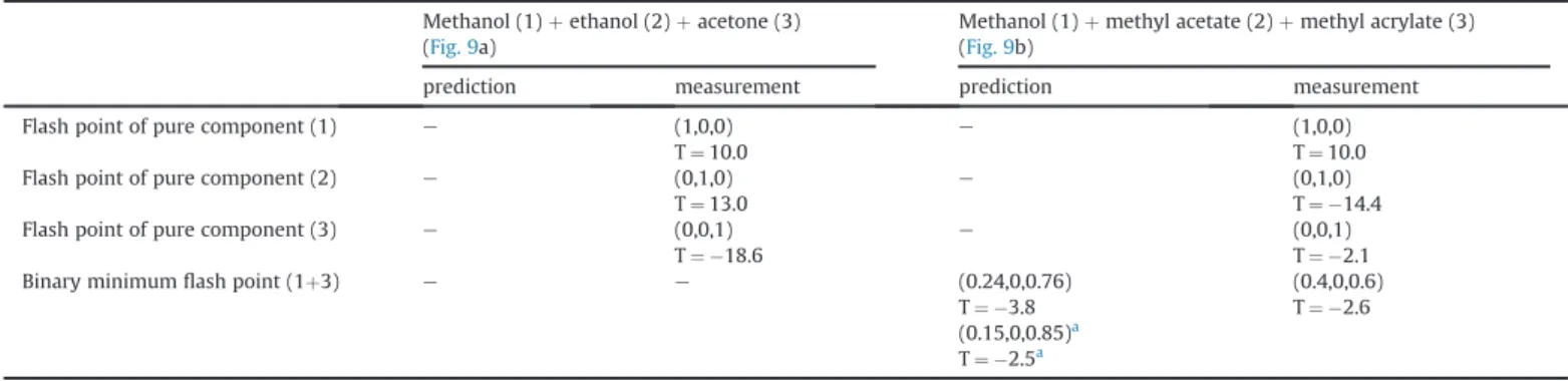
Fig. 9reports experimental and simulation results for the flash point of two ternary mixtures. In this figure, white squares

correspond to experimental data, bluedots correspond to predicted flash point based on UNIFAC Dortmund 93model. The critical points composition of the surfaces shown inFig. 9 are summarized in

Table 4.

Mixture methanol þ ethanol þ acetone has no binary minima/ maxima, and thus it belongs to type fp3.0.0e1. Mixture methanol þ methyl acetate þ methyl acrylate has no ternary critical point, but it presents one binary critical point. This critical point corresponds to a minimum flash point for the binary mixture methanol þ methyl acrylate, and it has a hyperbolic shape on the flash point surface inFig. 9b. Therefore, this mixture corresponds to category fp3.1.0e2. Note that, despite some deviation from the experimental data, all thermodynamic models predict the correct topology for both mixtures inFig. 9. The difference in composition exhibiting minimumflash point behavior between the measured data and the simulated one for IPA þ octane, ethanol þ octane, 2-butanol þ octane, cyclohexanol þ octane and methanol þ methyl acrylate, which are displayed inFigs. 8 and 9, is attributed to that

Table 4

Experimental and simulated molar compositions and flash point temperature (in,_{C) of critical points displayed inFig. 9[5].} Methanol (1) þ ethanol (2) þ acetone (3)

(Fig. 9a)

Methanol (1) þ methyl acetate (2) þ methyl acrylate (3)

(Fig. 9b)

prediction measurement prediction measurement

Flash point of pure component (1) e (1,0,0)

T ¼ 10.0

e (1,0,0)

T ¼ 10.0

Flash point of pure component (2) e (0,1,0)

T ¼ 13.0

e (0,1,0)

T ¼ $14.4

Flash point of pure component (3) e (0,0,1)

T ¼ $18.6

e (0,0,1)

T ¼ $2.1

Binary minimum flash point (1þ3) e e (0.24,0,0.76)

T ¼ $3.8 (0.15,0,0.85)a

T ¼ $2.5a

(0.4,0,0.6) T ¼ $2.6

a _{Simulation based on original UNIFAC model.}

Fig. 10. Experimental and predicted flash point surface of propyl acetate (1) þ IPA (2) þ octane (3).

the flash point values almost remain constant over a broad composition range, covering the measured and simulated compo-sitions [5].

Fig. 10shows experimental and predicted flash point tempera-tures for the mixture propyl acetate þ IPA þ octane. Differently fromFigs. 8 and 9, the data shown inFig. 10have not been pub-lished in other papers. The critical points composition of the surface of propyl acetate þ IPA þ octane are summarized inTable 5. The three binary constituents of propyl acetate þ IPA þ octane show minimum flash point behavior, with the experimental minimum flash point values of the binary constituents being 8.2,_{C, 8.1},_C,

6.3 ,_{C (Fig. 10). Blue dots predictions are based on the UNIFAC}

Dortmund 93 model; red dots predictions are based on the original UNIFAC model. The estimated minimum flash point of the ternary mixture is 5.5,_{C and 5.1},_{C at molar fractions of propyl acetate, IPA}

being 0.24, 0.36 and 0.18, 0.40 when based on UNIFAC-Dortmund 93 and original UNIFAC model, respectively. The experimental minimum value is 5.1,_{C at molar fractions of propyl acetate and IPA}

being 0.2 and 0.4 (Fig. 10). Hence, the topology for propyl acetate þ IPA þ octane corresponds to fp3.3.1e2.

The color maps shown inFig. 11a andFig. 11b were generated by simulation. For both presented mixtures, the model forecasts ternary minimum flash points, which have not yet been confirmed by experiments. These two mixtures are classified as type fp3.3.1e2.

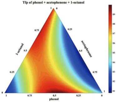
Fig. 12 shows the color map of the flash point temperature function for the mixture phenol þ acetophenone þ 1-octanol. The data has also been generated by simulation. We clearly see the hyperbolic behavior of the isotherms, which is an indicator of a ternary saddle point on the flash point temperature surface. Hence, this mixture belongs to fp3.3.1e4 type. The mixture's flash point

Fig. 11. Predicted flash point surface of two different mixtures (temperature scale in Celsius).

Fig. 12. ePredicted flash point surface for fp3.3.1e4 class phenol(1) þ acetophenone(2) þ 1-octanol(3) (temperature scale in Celsius). Table 5

Experimental and simulated molar composition and flash point temperature (in,_C) of critical points of propyl acetate þ IPA þ octane.

propyl acetate (1) þ IPA (2) þ octane (3)

prediction measurement

Flash point of pure component (1) e (1,0,0)

T ¼ 11.8

Flash point of pure component (2) e (0,1,0)

T ¼ 12.9

Flash point of pure component (3) e (0,0,1)

T ¼ 14.5 Binary minimum flash point (1 þ 2) (0.58,0.42,0)

T ¼ 8.2

(0.5,0.5,0) T ¼ 8.2 Binary minimum flash point (1 þ 3) (0.6,0, 0.4)

T ¼ 8.7

(0.6,0,0.4) T ¼ 8.1 Binary minimum flash point (2 þ3) (0,0.47, 0.53)

T ¼ 6.3

(0,0.6,0.4) T ¼ 6.3 Ternary minimum flash point (1 þ 2 þ 3) (0.24,0.36,0.40)

T ¼ 5.5

(0.2,0.4,0.4) T ¼ 5.1

behavior has not been confirmed by experiments yet. Table 6

summarizes the binary critical flash point simulation data for mixtures inFigs. 11 and 12. Flash point temperature for the indi-vidual components is given inTable 1, and data for the ternary critical points are presented inTable 2.

Unfortunately, lack of experimental data prevents us from making statistical studies on the most occurring classes.

5. Conclusion

By creating an auxiliary VLE system associated to a given closed-cup flash point system, it was possible to extend the main results of the VLE theory to propose a classification of the flash point tem-perature diagrams for ternary miscible flammable mixtures anal-ogous to the Serafimov isotherms classification [27]. This classification, shown inFig. 7, was used to analyze several ternary mixtures in section4.2. In some cases, it may also be able to predict the existence or the absence of critical and potentially dangerous behavior of the flash point temperatures, even without ternary experimental data. For instance, knowing that a ternary mixture does not present binary minimum flash points is enough to ensure that this mixture will not present a ternary minimum flash point. More experimental data on flash point temperatures of ternary mixtures is desirable to validate the proposed classification and to establish the flash point temperatures behavior for the most common mixtures. It could also enable to establish a statistical occurrence of each diagram that would help engineers to better assess potential risks. For example, statistical studies may show a strong correlation between some functional groups in a mixture and the corresponding type of flash point surface. During the screening of potential solvents for an extraction operation, engi-neers could use this to discard solvents which will form potential hazardous mixtures with the process' stream.

References

[1] T. Kletz, Learning from Accidents, 3 edition, Gulf Professional Publishing,

Oxford, 2001 (chapter 6).

[2] S. Mannan, Lees' Loss Prevention in the Process Industries, 4 edition,

Butter-worth-Heinemann, Oxford, 2012 appendix 1.

[3] L. Marmo, N. Piccinini, G. Russo, P. Russo, L. Munaro, Multiple tank explosions

in an edible-oil refinery plant: a case study, Chem. Eng. Technol. 36 (2013)

1131e1137.

[4] J. Gmehling, P. Rasmussen, Flash points of flammable liquid mixtures using

UNIFAC, Ind. Eng. Chem. Fundam. 21 (1982) 186e188.

[5] H.-J. Liaw, V. Gerbaud, Y.-H. Li, Prediction of miscible mixtures flash point

from UNIFAC group contribution methods, Fluid Phase Equil. 300 (2011)

70e82.

[6] H.-J. Liaw, Y.-Y. Chiu, A general model for predicting the flash point of miscible

mixture, J. Hazard Mater. 137 (2006) 38e46.

[7] H.-J. Liaw, C.-L. Tang, J.-S. Lai, A model for predicting the flash point of ternary

flammable solutions of liquid, Combust. Flame 138 (4) (2004) 308e319.

[8] H.-J. Liaw, V. Gerbaud, C.-Y. Chiu, Flash point for ternary partially miscible

mixtures of flammable solvents, J. Chem. Eng. Data 55 (2010) 134e146.

[9] H.-J. Liaw, V. Gerbaud, H.-T. Wu, Flash-point measurements and modeling for

ternary partially miscible aqueous-organic mixtures, J. Chem. Eng. Data 55

(2010) 3451e3461.

[10] H.-J. Liaw, T.-P. Tsai, Flash points of partially miscible aqueous-organic

mix-tures predicted by UNIFAC group contribution methods, Fluid Phase Equil. 345

(2013) 45e49.

[11] H.-J. Liaw, T.-P. Tsai, Flash-point estimation for binary partially miscible

mixtures offlammable solvents by UNIFAC group contribution methods, Fluid

Phase Equil. 375 (2014) 275e285.

[12] V.N. Kiva, E.K. Hilmen, S. Skogestad, Azeotropic phase equilibrium diagrams: a

survey, Chem. Eng. Sci. 58 (2003) 1903e1953.

[13] H.-J. Liaw, H.-Y. Chen, Study of two different types of minimum flash-point

behavior for ternary mixtures, Ind. Eng. Chem. Res. 52 (2013) 7579e7585.

[14] S. da Cunha, H.-J. Liaw, V. Gerbaud, On the relation between azeotropic

behavior and minimum/maximumflash point occurrences in binary mixtures

of flammable compounds, Fluid Phase Equil. 452 (2017) 113e134.

[15] M.F. Doherty, J.D. Perkins, On the Dynamics of Distillation Processes - III. The

topological structure of ternary residue curve maps, Chem. Eng. Sci. 34 (1979)

1401e1414.

[16] M.D. Koretsky, Engineering and Chemical Thermodynamics, 2 edition, Wiley,

2013 (chapter 7).

[17] J.M. Prausnitz, R.N. Lichtenthaler, E.G. Azevedo, Molecular Thermodynamics of

Fluid Phase Equilibria, 3 edition, Prentice Hall, New Jersey, 1999 (chapter 2).

[18] M.F. Doherty, J.D. Perkins, On the dynamics of distillation processes - I. The

simple distillation of multicomponent non-reacting, homogeneous liquid

mixtures, Chem. Eng. Sci. 33 (1978) 281e301.

[19] V.T. Zharov, L.A. Serafimov, Physicochemical Foundations of Simple

Distilla-tion and RectificaDistilla-tion, Chemistry Publishing Co., Leningrad, 1975 (in Russian).

[20] N. Shcherbakova, V. Gerbaud, I. Rodriguez-Donis, On the Riemannian

struc-ture of the residue curves maps, Chem. Eng. Res. Des. 99 (2015) 87e96.

[21] F.A.H. Schreinemakers, Dampfdrucke ternaer gemische. Theoretischer teil:

erste abhandlung, Zeitrschrift fuer Physikalische Chemie 36 (1901) 257e289

(in German).

[22] D.B. van Dongen, M.F. Doherty, On the dynamics of distillation process e V.

The topology of the boiling point surface and its relation to azeotropic

distillation, Chem. Eng. Sci. 39 (1984) 883e892.

[23] J.W. Milnor, Topology from the Differentiable Viewpoint, Univ. Virginia Press,

Charlottesville, 1965.

[24] Y.V. Gurikov, Structure of the vaporeliquid equilibrium diagrams of ternary

homogeneous solutions, Russ. J. Phys. Chem. 32 (1958) 1980e1996 (abstract

in English) (in Russian).

[25] N. Shcherbakova, I. Rodriguez-Donis, J. Abildskov, V. Gerbaud, A novel method

for detecting and computing univolatility curves in ternary mixtures, Chem.

Eng. Sci. 173 (2017) 21e36.

[26] E.K. Hilmen, V.N. Kiva, S. Skogestad, Topology of ternary VLE diagrams:

elementary cells, AIChE J. 48 (2002) 752e759.

[27] L.A. Serafimov, V.M. Raeva, V.N. Stepanov, Classification of scalar property

isoline diagrams of homogeneous ternary mixtures, Theor. Found. Chem. Eng.

46 (2012) 221e232.

[28] H.-J. Liaw, W.H. Lu, V. Gerbaud, C.C. Chen, Flash-point prediction for binary

partially miscible mixtures of flammable solvents, J. Hazard Mater. 153 (3)

(2008) 1165e1175.

[29] N.D.D. Carareto, C.Y.C.S. Kimura, E.C. Oliveira, M.C. Costa, A.J.A. Meirelles, Flash

points of mixtures containing ethyl esters or ethylic biodiesel and ethanol,

Fuel 96 (2012) 319e326.

[30] D.-M. Ha, S. Lee, M.-H. Back, Measurement and estimation of the lower flash

points for the flammable binary systems using a Tag open cup tester, Kor. J.

Chem. Eng. 24 (4) (2007) 551e555.

[31] A.Z. Moghaddam, A. Rafiei, T. Khalili, Assessing prediction models on

calcu-lating the flash point of organic acid, ketone and alcohol mixtures, Fluid Phase

Equil. 316 (2012) 117e121.

[32] L.Y. Phoon, A.A. Mustaffa, H. Hashim, R. Mat, A review of flash point prediction

models for flammable liquid mixtures, Ind. Eng. Chem. Res. 53 (2014)

12553e12565.

[33] X. Liu, Z. Liu, Research progress on flash point prediction, J. Chem. Eng. Data 55

(2010) 2943e2950.

[34] American Society for Testing and materials, Standard test method for flash

point by tag closed tester, ASTM D 56 (1993).

[35] Simulis Thermodynamics®, 2010.http://www.prosim.net. [36] Alfa Aesar.https://www.alfa.com. Last accessed 23 July 2017.

[37] DIPPR- Design Institute for Physical Properties.http://www.aiche.org/dippr.

[38] B.E. Poling, J.M. Prausnitz, J.P. O'Connell, The Properties of Gases and Liquids, 5

edition, McGraw-Hill, New York, 2001.

[39] J. Gmehling, U. Onken, W. Arlt, Vaporeliquid Equilibrium Data Collection, vol.

1, DECHEMA, Frankfurt, 1978 part 2b.

Table 6

Simulated molar composition and flash point temperature (in,_{C) of binary critical} points displayed inFigs. 11 and 12.

Fig. 11a Fig. 11b Fig. 12

(1þ2) (0.4,0.6,0) T ¼ $2.2 (0.5,0.5,0) T ¼ 3.8 (0.45,0.55,0) T ¼ 90.0 (1þ3) (0.35,0,0.65) T ¼ 1.9 (0.5,0,0.5) T ¼ 4.4 (0.26,0,0.74) T ¼ 89.3 (2þ3) (0,0.5,0.5) T ¼ $1.3 (0,0.6,0.4) T ¼ 8.2 (0,0.65,0.35) T ¼ 80.8