Minimal controllability time for the heat equation under unilateral state or control constraints

HAL Id: hal-01457931

https://hal.archives-ouvertes.fr/hal-01457931

Submitted on 6 Feb 2017

HAL is a multi-disciplinary open access

archive for the deposit and dissemination of

sci-entific research documents, whether they are

pub-lished or not. The documents may come from

L’archive ouverte pluridisciplinaire HAL, est

destinée au dépôt et à la diffusion de documents

scientifiques de niveau recherche, publiés ou non,

émanant des établissements d’enseignement et de

Minimal controllability time for the heat equation under

unilateral state or control constraints

Jérôme Lohéac, Emmanuel Trélat, Enrique Zuazua

To cite this version:

Jérôme Lohéac, Emmanuel Trélat, Enrique Zuazua. Minimal controllability time for the heat equation

under unilateral state or control constraints. Mathematical Models and Methods in Applied Sciences,

World Scientific Publishing, 2017, 27 (9), pp.1587–1644. �10.1142/S0218202517500270�. �hal-01457931�

Minimal controllability time for the heat equation under

unilateral state or control constraints

J´

erˆ

ome Loh´

eac

Emmanuel Tr´

elat

Enrique Zuazua

February 6, 2017

Abstract

The heat equation with homogeneous Dirichlet boundary conditions is well known to pre-serve nonnegativity. Besides, due to infinite velocity propagation, the heat equation is null-controllable within arbitrary small time, with controls supported in any arbitrarily open subset of the domain (or its boundary) where heat diffuses.

The following question then arises naturally: can the heat dynamics be controlled from a positive initial steady-state to a positive final one, requiring that the state remains nonneg-ative along the controlled time-dependent trajectory? We show that this state-constrained controllability property can be achieved if the control time is large enough, but that it fails to be true in general if the control time is too short, thus showing the existence of a positive minimal controllability time. In other words, in spite of infinite velocity propagation, realizing controllability under the unilateral nonnegativity state constraint requires a positive minimal time.

We establish similar results for unilateral control constraints.

We give some explicit bounds on the minimal controllability time, first in 1D by using the sinusoidal spectral expansion of solutions, and then in multi-D on any bounded domain. We illustrate our results with numerical simulations, and we discuss similar issues for other control problems with various boundary conditions.

Contents

1 Introduction 2

2 Minimal time for the Dirichlet controlled 1D heat equation under

nonneg-ativity constraints 5

2.1 Main results . . . 5

2.2 Weak solutions with controls that are Radon measures . . . 7

2.3 Proof of Theorem 1 . . . 8

∗_{LUNAM Universit´e, IRCCyN UMR CNRS 6597 (Institut de Recherche en Communications et}

Cy-bern´etique de Nantes), Ecole´ des Mines de Nantes, 4 rue Alfred Kastler, 44307 Nantes, France ([email protected]).

†_{Sorbonne Universit´es, UPMC Univ Paris 06, CNRS UMR 7598, Laboratoire Jacques-Louis Lions, F-75005,}

Paris, France ([email protected]).

‡_{DeustoTech, Fundaci´on Deusto, Avda Universidades, 24, 48007, Bilbao - Basque Country - Spain}

([email protected])

§_{Departamento de Matem´aticas, Universidad Aut´onoma de Madrid, Cantoblanco, 28049 Madrid - Spain} ¶_{Facultad Ingenier´ıa, Universidad de Deusto, Avda. Universidades, 24, 48007, - Basque Country - Spain}

∥_{Sorbonne Universit´es, UPMC Univ Paris 06, CNRS UMR 7598, Laboratoire Jacques-Louis Lions, F-75005,}

2.4 Proof of Proposition 1 . . . 9

2.5 Proof of Theorem 2 . . . 11

2.6 Lower estimates of the minimal time for a constant initial datum . . . 12

3 Minimal time for Dirichlet controlled multi-D heat equations under non-negativity constraints 14 3.1 Heat equation in a ball with nonnegative Dirichlet controls . . . 14

3.2 General domain and nonnegativity state constraint . . . 18

3.3 Relationship with the viscous Hamilton-Jacobi equation . . . 20

4 Generalizations 20 4.1 Mixed Dirichlet-Neumann boundary conditions. . . 20

4.2 Neumann control under nonnegativity state constraints. . . 21

4.3 Internal control with Neumann boundary conditions. . . 24

4.4 Neumann boundary control with control constraints in 1D . . . 25

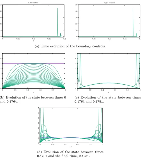
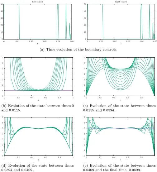
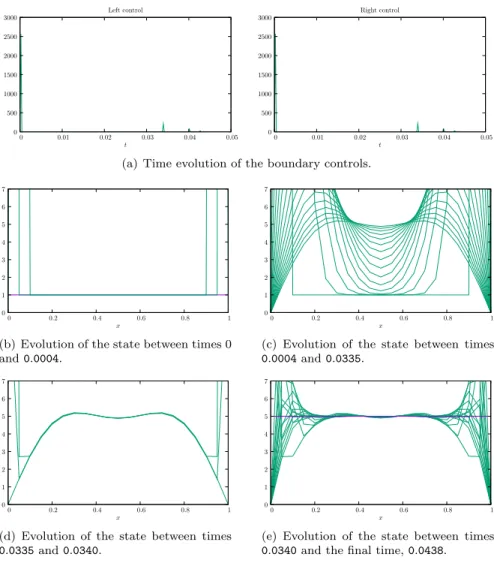
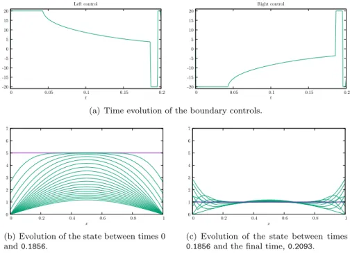
5 Numerical simulations 27 5.1 Dirichlet boundary controls with nonnegativity control constraints . . . 27

5.2 Neumann controls and state constraints . . . 33

5.3 Convergence result for the minimal time . . . 35

6 Conclusion, open problems and perspectives 36

1

Introduction

This work is devoted to analyze the controllability properties on the heat equation under nat-ural unilateral constraints on the state. The free heat equation, in the absence of control and, for instance, for homogeneous Dirichlet boundary conditions, is well known to preserve non-negativity. Besides, due to infinite velocity propagation, the heat equation is null-controllable within arbitrary small time with controls acting on an arbitrarily small open subset of the domain (of its boundary) where heat propagates.

The following question then arises naturally: if the initial datum and the final target are positive steady-states, can the heat dynamics be controlled under a nonnegativity state constraint along the whole trajectory?

In this paper, we present two types of complementary results exhibiting a “waiting or minimal time phenomenon”. Roughly, we show that, given positive initial and final steady-states, the system can be controlled while preserving nonnegativity of the state provided that the time horizon[0, T ] be long enough. This is not surprising: in fact, when the time-interval is long, we expect the control property to be achieved with controls of small amplitude, thus ensuring small deformations of the state and, in particular, preserving its positivity. As we will see, it suffices that the target be positive, regardless of the sign of the initial datum, to ensure that the controls are positive as well. If, in addition, the initial datum is positive as well, the positivity of the control ensures positivity of the state everywhere.

Maybe more surprisingly, we also prove that, if the time-interval is too short, then the controllability property fails under the nonnegativity state-constraint. In other words, even if the initial datum and final steady target are positive, nonnegativity cannot be preserved along the controlled trajectory if the time horizon is too short: in spite of infinite velocity propaga-tion, controlling the system then requires to violate the natural nonnegativity constraint on the state. This means, roughly speaking, that the necessary action of the control to avoid the state to cross the limit established by the constraint, is an impediment for the state to reach the target, unless the control time horizon is long enough.

This negative result, which is counterintuitive to some extent, is a serious warning for the practical use of existing controllability results, that are valid within arbitrarily short time since, as often in applications, state-constraints need to be preserved along controlled trajectories.

This is the case, for instance, when the heat equation or, more generally, the diffusive system under consideration, models the propagation of a population density, as in the context of population dynamics.

We mainly focus on the heat equation with Dirichlet boundary control. To simplify the presentation, we first analyze the 1D heat equation although, as we shall see, the results can then be extended to the multi-D case.

To begin with, we consider the 1D heat equation with Dirichlet boundary controls: ∂ty(t, x) = ∂2xy(t, x) (t > 0, x ∈ (0, 1)), (1a)

y(t, 0) = u0(t) (t > 0), (1b)

y(t, 1) = u1(t) (t > 0), (1c)

with constant initial condition y(0, x) = y0 > 0 (steady-state). The controls are represented by the time-dependent functions u0(t) and u1(t) that act on the system at the boundary

points x = 0 and x = 1, respectively. Here, we assume that the initial state is a positive constant y0_{> 0, thus a steady-state of the system that can be sustained with constant controls}

u0(t) ≡ u1(t) ≡ y0.

Given a constant steady-state target y1 _{> 0 (steady-state sustainable with the constant}

controls u0(t) ≡ u1(t) ≡ y1), as mentioned above, whatever the time of control T > 0 is, we

know that there exist controls u0 and u1 in L2(0, T ) steering the system to y1 in time T , i.e.,

such that

y(T, x) = y1 (x ∈ [0, 1] a.e.). (2) The problem we analyze is whether the controls u0 and u1 can be chosen so that the

solu-tion remains nonnegative along the time interval, i.e., whether the following unilateral state constraint can be satisfied:

y(t, x) ⩾ 0, ∀t ∈ (0, T ), x ∈ (0, 1). (3) Of course we are only interested in the nontrivial case where y1≠ y0. Otherwise, when y1= y0 the trivial trajectory y≡ y0= y1 solves the problem with constant controls u0≡ u1≡ y0= y1.

In this paper, we establish two types of results:

• Controllability can be achieved while preserving nonnegativity (3) if T> 0 is large enough; • Controllability fails if T > 0 is too small; more precisely, there exists T (y0

, y1) > 0 such that, for every T ∈ (0, T (y0, y1)), there do not exist any controls u0 and u1 such that

the solution y of the heat equation satisfies (2) while satisfying the state constraint (3). This means that there is a positive minimal time, or waiting time.

In the absence of state-constraints, it is well known that, given any T > 0, there exist controls such that the solution y of the heat equation reaches y1 in time T (see for instance [25, §11.5] and see references therein), and this result is even valid for much more general heat equations with various types of controls and boundary conditions in multi-D. But it is important to emphasize that usual results of the literature do not take into consideration the objective of preserving state-constraints, and actually the numerical results that one can find in the existing literature show that the corresponding controls and controlled trajectories enjoy significant oscillations (see [16]), thus showing the difficulties that may arise under state-constraints.

Our result ensuring that constrained controllability can be achieved if T is large enough can be roughly proved as follows. When T is large, the cost of control tends to zero. In fact in the present setting of Dirichlet boundary controls it can be easily proved that the cost of control can be made exponentially small as T→ +∞, and that for T large enough the control can be made arbitrarily small in L∞

norm. Moreover, the comparison or maximum principle for the heat equation guarantees that the controlled trajectory remains in a tubular neighborhood of y0 _{and y}1 _{all along the time horizon [0, T ] and, in particular, preserves the nonnegativity}

constraint when y0 and y1are positive. Note that this argument fails in short time when the size of controls may become large.

To prove that, if the control time T is too small, then nonnegativity of the solution cannot be guaranteed in general (thus, there is a positive “minimal” or “waiting time”), we use the classical maximum or comparison principle for the heat equation. Since y0> 0, controllability under the state constraint (3) is in fact equivalent to the apparently weaker property

u0(t) = y(t, 0) ⩾ 0 and u1(t) = y(t, 1) ⩾ 0 (t ∈ (0, T ) a.e.). (4)

Indeed, when the nonnegativity state constraint (3) is satisfied, the boundary constraint (4) is satisfied too. On the other hand, the latter and the positivity of the initial state suffice to show that the state is nonnegative everywhere. This shows the equivalence between the problems of control under nonnegative state and control constraints, for the heat equation with Dirichlet controls.

In view of this, in some particular cases, it is easy to see that a positive minimal time is required for controlling the system under nonnegativity state constraints. This occurs if the final target is smaller than the initial datum, i.e., if 0< y1 < y0 (recall that y0 and y1 are constant). Indeed, we infer from the maximum or comparison principle for the heat equation that, whatever the controls u0 and u1 are, if the solution y satisfies the nonnegativity state

constraint (3), then, due to (4), we must have

y(t, x) ⩾ ˜y(t, x) (t ∈ (0, T ), x ∈ (0, 1) a.e.), where ˜y is solution of ∂t˜y(t, x) = ∂ 2 xy˜(t, x) (t > 0, x ∈ (0, 1)), ˜ y(t, 0) = ˜y(t, 1) = 0 (t > 0), ˜ y(0, x) = y0 (x ∈ (0, 1)), and then, since ˜y(0, x) ⩾ y0sin(πx), we infer that

˜

y(t, x) ⩾ y0exp(−π2t) sin(πx),

sin(π ⋅) being the first eigenfunction of the Dirichlet-Laplacian in (0, 1). It follows that sup

x∈[0,1]

y(t, x) ⩾ y0exp(−π2t),

and thus, if 0< y1 < y0, then there exists a positive minimal time T(y0, y1) > 0 to steer the system from y0 to y1, and we have

T(y0, y1) ⩾ 1 π2ln(

y0 y1) .

In the present paper, we will also establish that a similar but much less obvious phenomenon occurs when y1> y0> 0. This fact, contrarily to the previous observation corresponding to the case where 0< y1< y0, is quite surprising because, at the first view, nothing prevents y from increasing as fast as needed under the action of nonnegative controls. To handle this case, we will need to study more deeply the Dirichlet control problem, using spectral expansions of solutions. This will be done in Section2, where moreover the initial datum y0 _{can be any}

function in L2(0, 1).

In Section3, we extend these results to the multi-dimensional case. As mentioned above, the fact that constrained controllability can be achieved in long time intervals is a consequence of classical results on the decay of the control cost as T→ +∞, and thus it is easy to extend to the multi-D setting. In contrast, the 1D proof of the necessity of a waiting time uses explicit properties of the 1D Laplacian. We first extend this result to the multi-D ball, by using the explicit form of radially symmetric eigenfunctions and getting explicit lower bounds on the waiting time. Once this is done, the result is extended to any other domain by comparison with the largest ball included in the domain. Note that, in Section3.3, we present an interesting

remark done by M. Tucsnak [24], indicating that the waiting time phenomenon for the control of the linear heat equation under nonnegativity state-constraints is related to that of [17] on the control of the viscous Hamilton-Jacobi equations.

In Section4, we then consider similar issues in various other situations. First, in the case of Neumann boundary control, the same arguments lead to a waiting time principle under state-constraints. The reason is the same: if the state remains positive, it can always be viewed as a controlled trajectory with positive Dirichlet controls. But we also consider, among others, the case of interior controls applied in a subdomain of the region where heat diffuses.

In Section5, we present some numerical simulations that confirm our analytical results, shedding new light on the nature of the constrained controls in the minimal control time and raising new questions.

We conclude with a section devoted to open problems and some possible extensions.

2

Minimal time for the Dirichlet controlled 1D heat

equation under nonnegativity constraints

In this section, we consider the 1D heat equation (1) with Dirichlet boundary controls. We assume that the final target y1 _{is a positive constant, which corresponds to a steady-state of}

the system. More generally than in the previous section, the initial datum y0can now be any element of L2(0, 1).

We have seen in Section1that, if y0> 0, then controllability under the nonnegativity state constraint (3) is equivalent to controllability under the nonnegativity control constraints (4). This is why, in this section, we consider unilateral nonnegativity control constraints. But all results hereafter are then valid as well for unilateral nonnegativity state constraints.

2.1

Main results

We consider an arbitrary y0 ∈ L2(0, 1) (without any sign requirement), and we consider the problem of steering the heat equation (1) from y0 _{to the positive steady-state y}1_{, under the}

unilateral control constraints

u0(t) ⩾ 0, u1(t) ⩾ 0, a.e. t∈ (0, T ). (5)

Our first main result states the existence of such controls for a large enough time T .

Theorem 1. Let y0 ∈ L2(0, 1) be arbitrary, and let y1 > 0 be a positive constant, such that y0 ≠ y1. There exist T > 0, depending on the initial and final data y0, y1, and controls u0 ∈ L1(0, T ) and u1 ∈ L1(0, T ), satisfying the nonnegativity constraints (5), such that the

corresponding solution y of (1), with y(0) = y0, satisfies y(T ) = y1.

Theorem1is proved in Section2.3. Note that, as we will see in the proof, for T > 0 large enough the controls are actually positive (and y0 need not be nonnegative), due to positivity of the target at the final time.

Remark 1. We can actually state the following result of controllability to trajectories, slightly extending Theorem1:

Let ¯y0 _{∈ L}2_{(0, 1) and let ¯u}

0 and ¯u1 in L1loc([0, +∞)) be arbitrary. Let ¯y be the

solution of (1) corresponding to the initial condition ¯y(0) = ¯y0 and to the controls ¯

u0 and ¯u1. We assume that there exists ν> 0 such that ¯ui(t) ⩾ ν, for i = 0, 1 and

for almost every t∈ [0, +∞).

Then, for every y0 ∈ L2(0, 1), there exist T > 0 and nonnegative controls u0 ∈

L1(0, T ) and u1 ∈ L1(0, T ) such that the solution y of (1) corresponding to the

This result is an extension of Theorem1(where ¯y≡ y1 _{and ¯u}

0= ¯u1= 0). The proof is similar

to the one of Theorem1, by subtracting ¯y to y so we have to steer y0− ¯y0 to 0 with control v= u − ¯u and we prove that there exists a control v ∈ H1(0, T ) (for T large enough) satisfying v(t) ⩾ −ν, i.e., u(t) ⩾ 0.

Let us now study the minimal time required to steer y0 to y1 in Theorem 1, and prove that it is positive. We define the minimal controllability time

T(y0, y1) = inf {T > 0, ∃u0, u1∈ L1(0, T ) s.t. u0⩾ 0, u1⩾ 0 and y(0) = y0, y(T ) = y1} .

It is defined here with controls in L1(0, T ), but it could also be defined with other functional control spaces. However, on the one part, the arguments we shall develop, based on spectral expansions, lead to bounds in L1(0, T ) that are uniform with respect to T > T (y0, y1) and, consequently, are valid in the space of measures for the minimal time T(y0, y1). On the other part, the following result shows that, if controllability can be achieved in time T with controls in L1(0, T ), then it can also be achieved in time T +τ with τ > 0 arbitrarily small, with controls that are arbitrarily more regular.

Proposition 1. Let y0∈ L2(0, 1) be arbitrary, and let y1> 0 be a positive constant. Let T > 0 be such that there exist controls u0∈ L1(0, T ) and u1∈ L1(0, T ), satisfying the nonnegativity

constraints (5), for which the corresponding solution y of (1), with y(0) = y0, satisfies y(T ) = y1.

Now, let n∈ IN∗

and let τ> 0 be arbitrary. Then there exist controls ˜u0∈ Cn([0, T +τ]) and

˜

u1 ∈ Cn([0, T + τ]), satisfying the nonnegativity constraints (5), such that the corresponding

solution ˜y of (1), with ˜y(0) = y0_{, satisfies ˜y(T + τ) = y}1_.

This result will be proved in Section2.4. Our second main result is the following.

Theorem 2. Given any y0∈ L2(0, 1) and any positive constant y1> 0 such that y0≠ y1, we have T(y0, y1) > 0.

Moreover, there exist nonnegative controls u₀, u₁ ∈ M(0, T (y0, y1)) (the space of Radon measures) steering the heat equation (1) from y0 to y1 in time T(y0, y1).

This result states not only that the minimal time required to steer y0_{to y}1 _{in Theorem1}

is positive, but also that controllability exactly at the minimal time T(y0, y1) can be achieved with controls that are Radon measures. We do not know whether they can be taken more regular or not. When controls are Radon measures, the concept of weak solution of the heat equation (defined by transposition) is recalled in Section2.2.

Remark 2. Given any T > T (y0, y1), by definition there exist controls u0and u1in L1(0, T ),

satisfying the nonnegativity constraints (5), steering the heat equation (1) from y0to y1in time T . We claim that, if y0 is symmetric with respect to x= 1/2, meaning that y0(x) = y0(1 − x) for almost every x∈ [0, 1], then we can take u0= u1.

Remark 3. As we will see in the proof, the fact that T(y0_{, y}1_{) > 0 under the control}

con-straints (5) is actually due to the positivity of the constant target y1, independently of the initial datum y0.

Theorem2and the above remarks are proved in Section2.5. As discussed previously, this result yields a positive minimal time as well for the control of the Dirichlet heat equation under nonnegativity state constraints.

In Section2.6further, we provide lower estimates of the minimal time T(y0, y1) when the initial datum y0 _{is a positive constant.}

Before proving Theorem1, Proposition1and Theorem2, let us recall hereafter the notion of weak solutions with controls that are Radon measures.

2.2

Weak solutions with controls that are Radon measures

We recall here the concept of solution y of the Dirichlet control problem (1) with controls in the (Banach) space of Radon measuresM(0, T ) endowed with the norm

∥µ∥M(0,T )= sup {∫

[0,T ]

ϕ(t) dµ(t) ∣ ϕ ∈ C0([0, T ], IR), max

[0,T ]∣ϕ∣ = 1} .

Solutions of the Dirichlet control problem (1) with controls in M(0, T ) are then defined by transposition: given y0∈ L2(0, 1), given u0and u1inM(0, T ), we say that y is a weak solution

of (1) if ∫₀T∫₀1(−∂tϕ(t, x) − ∂x2ϕ(t, x)) y(t, x) dx dt − ∫ 1 0 y0(x)ϕ(0, x) dx = ∫_{[0,T ]}∂xϕ(t, 0) du0(t) − ∫ [0,T ] ∂xϕ(t, 1) du1(t), (6)

for every ϕ∈ C2([0, T ] × [0, 1]) satisfying ϕ(t, 0) = ϕ(t, 1) = ϕ(T, x) = 0 for all (t, x) ∈ [0, T ] × [0, 1].

Existence and uniqueness of solutions y∈ C0([0, T ]; H−s(0, 1)) of (1), for s> 3/2, with con-trols in L1_{(0, T ), is obtained by classical duality and transposition arguments. This regularity}

property suffices to give a sense to the trace of the solution at t= T and to the controllability problem when the controls are in L1_{(0, T ). To check this regularity property, it suffices to}

observe that the solutions of the forced adjoint problem

−∂tϕ(t, x) = ∂x2ϕ(t, x) + f(t, x) (t ∈ (0, T ), x ∈ (0, 1)),

ϕ(t, 0) = ϕ(t, 1) = 0 (t ∈ (0, T )), ϕ(T, x) = 0 (x ∈ (0, 1)),

satisfy ϕx(0, t), ϕx(1, t) ∈ C0([0, T ]) when f ∈ L1(0, T ; Hs(0, 1)) with s > 3/2. This is due to

the fact that ϕ∈ C0([0, T ]; Hs(0, 1)) and that Hs(0, 1) is continuously embedded in C1(0, 1) when s> 3/2.

When the controls are taken to be inM(0, T ), by density arguments, the solution defined by transposition can be shown to be in L∞

(0, T ; H−s_{(0, 1)) for every s > 3/2. In this case the}

trace of the solution at t= 0 and t = T has to be understood in the sense of (6).

The spectral expansion of the solutions of the controlled problem provides an alternative way of representing the solutions given by transposition as above. Indeed, consider the eigen-basis (√2 sin(nπx))n∈IN∗ of the Dirichlet-Laplacian. For every t ⩾ 0 and every n ∈ IN

∗ , we set yn(t) = ∫ 1 0 y(t, x) sin(nπx) dx. Then, by integrating by parts, we easily have

˙

yn(t) = nπ (u0(t) − (−1)nu1(t)) − n2π2yn(t),

with yn(0) = ∫ 1 0

y0(x) sin(nπx) dx = yn0, and thus,

yn(t) = e−n

2_π2_t

y0n+ nπ ∫ [0,t]

e−n2π2(t−s)d(u0− (−1)nu1) (s).

Then, when the controls u0and u1 belong toM(0, T ), at the final time t = T we have

yn(T ) = e−n

2_π2_T

y0n+ nπ ∫ [0,T ]

e−n2π2(T −s)d(u0− (−1)nu1) (s),

which is well defined in view of the fact that e−n2π2(T −s) depends continuously on s∈ (0, T ). This gives a sense to the trace of the transposition solution at the final time t= T .

2.3

Proof of Theorem

1

Let us first mention that this result directly follows from [18, Theorem 4.1, b]. However, we provide a sketch of the proof, showing moreover that the controls can even be chosen in H1_{(0, T ).}

First of all, observe that, by subtracting y1, it suffices to prove that there exists a time T > 0 and controls u0 and u1 in H1(0, T ) satisfying u0(t) > −y1 and u1(t) > −y1 on [0, T ],

such that the corresponding solution y of (1), with y(0) = y0− y1, satisfies y(T ) = 0.

According to [8, Theorem 3.3], for any T > 0 there exist controls u0, u1 ∈ H1(0, T ) such

that the solution y of (1) for any initial condition in L2(0, 1) satisfies y(T, ⋅) = 0.

Note that, at this point, we use the classical controllability property for the 1D heat equation without any constraint. Our goal is to show that, if the control time T > 0 is large enough, then the controls can be taken such that u0(t) > −y1and u1(t) > −y1for almost every

t∈ [0, T ].

It is well known (see [14]) that controllability with controls in H1(0, T ), without any con-straint, is equivalent to an observability inequality, namely to the existence of an observability constant c(T ) > 0 such that

∥z(0, ⋅)∥2

L2(0,1)⩽ c(T ) (∥∂xz(⋅, 0)∥2H−1(0,T )+ ∥∂xz(⋅, 1)∥2H−1(0,T )) ,

for any solution of the adjoint system −∂tz(t, x) = ∂

2

xz(t, x) (t > 0, x ∈ (0, 1)), (7a)

z(t, 0) = z(t, 1) = 0 (t > 0), (7b) such that z(T ) ∈ L2(0, 1). Actually, the controllability (and equivalently, the observability of the adjoint system) being true on any time interval(τ, T ), we also have

∥z(τ, ⋅)∥2

L2_(0,1)⩽ c(T − τ) (∥∂xz(⋅, 0)∥2H−1(τ,T )+ ∥∂xz(⋅, 1)∥2H−1(τ,T )) .

Using a spectral expansion and the Parseval equality, we have the estimate ∥z(0, ⋅)∥2

L2(0,1)⩽ e −2π2τ

∥z(τ, ⋅)∥2 L2(0,1)

for every 0< τ < T , and hence ∥z(0, ⋅)∥2

L2_(0,1)⩽ e−2π 2_τ

c(T − τ) (∥∂xz(⋅, 0)∥2H−1(0,T )+ ∥∂xz(⋅, 1)∥2H−1(0,T )) .

By duality, this means that the controls u0 and u1 can be chosen such that

∥ui∥2H1(0,T )⩽ e −2π2τ

c(T − τ) ∥y0− y1∥2L2(0,1) i= 0, 1,

for any 0< τ < T . By continuous embedding of H1(0, T ) into L∞(0, T ),

∥ui∥2L∞(0,T )⩽ C∥ui∥H1(0,T )⩽ C(T )e −2π2τ

c1(T − τ)∥y0− y1∥2L2(0,1) i= 0, 1,

with C(T ) the constant of the continuous embedding. Hence, taking τ = T /2 and observing that c1(T − τ) = c1(T /2) is monotonic decreasing with respect to T and observing that C(T )

is bounded by a polynomial function, we have, for T large enough, ∥u0∥L∞(0,T ),∥u1∥L∞(0,T )< y

1

2.4

Proof of Proposition

1

First of all according to Theorem1, for T large enough there exist controls u0∈ L1(0, T ) and

u1 ∈ L1(0, T ), satisfying the constraints (5), such that the corresponding solution y of (1),

with y(0) = y0_{, satisfies y(T ) = y}1_.

As in the proof of Theorem1, it suffices to prove that there exist controls ˆv0 and ˆv1 in

Cn([0, T +τ]) satisfying ˆv0(t) > −y1and ˆv1(t) > −y1on[0, T +τ], such that the corresponding

solution ˆy of (1), with ˆy(0) = y0− y1, satisfies ˆy(T + τ) = 0. Note first that the controls v0= u0−y1and v1= u1−y1satisfy v0(t) > −y1and v1(t) > −y1on[0, T ], and the corresponding

solution y of (1), with y(0) = y0− y1, satisfies y(T ) = 0.

The idea of the proof is the following. Firstly, we will smoothen the controls v0 and v1.

Then the solution of the heat equation at time T , obtained with these smooth controls, will be some ¯y1, close to 0. Secondly, we will steer ¯y1to the target 0 in time τ with smooth controls. Of course, in order to ensure that the controls steering ¯y1 to 0 in time τ are greater than−y1, the smaller τ is, the more ¯y1 must be close to 0.

For every ε > 0, by a density argument, there exist ¯vε0 and ¯v ε

1 in C

∞(0, T ) such that

∥vi− ¯vεi∥L1_{(0,T )}< ε, and such that all time derivatives of ¯v0ε and ¯v1ε vanish at time T . Since

v0⩾ −y1 and v1⩾ −y1, we assume moreover that ¯vε0⩾ −y 1

and ¯vε1⩾ −y 1

.

The well posedness of the heat equation for L1 Dirichlet boundary conditions (see Sec-tion2.2) ensures that the solution ¯y of (1), with ¯y(0) = y0− y1 and boundary controls ¯vε0 and

¯ vε

1, satisfies∥¯y(T )∥H−2(0,1)⩽ C1ε, for some C1> 0.

Set ¯y1 = ¯y(T ) ∈ H−2(0, 1) and set ¯y0 = y0(τ/2) ∈ L2(0, 1), where y0 is the solution of (1)

corresponding to the initial condition y0(0) = ¯y1 and to null boundary controls. Then there

exists C2(τ) > 0 such that ∥¯y0∥L2(0,1)⩽ C2(τ)∥¯y1∥H−2(0,1), i.e.,∥¯y0∥L2(0,1)⩽ C1C2(τ)ε.

The aim is now to steer ¯y0 to 0 with controls ˜v0and ˜v1 in Cn([0, τ/2]) such that

˜

vi(t) ⩾ −y1 (t ∈ [0, τ/2]) and vi(0) = ⋅ ⋅ ⋅ = v(n)_i (0) = 0 (i = 0, 1).

This is a consequence of the following lemma. Lemma 1. Let y0 _{∈ L}2_{(0, 1), let n ∈ IN}∗

and let τ > 0 be arbitrary. There exist controls v0 and v1 in Cn([0, τ]) satisfying vi(0) = ⋅ ⋅ ⋅ = v(n)_i (0) = 0, for i = 1, 2, such that the

corre-sponding solution of (1) (with controls v0 and v1) with initial condition y(0) = y0 satisfies

y(τ) = 0. Moreover, v0 and v1 can be chosen such that

max(∥v0∥L∞(0,τ ),∥v1∥L∞(0,τ )) ⩽ κn(τ)∥y0∥L2_(0,1), for some κn(τ) > 0 only depending on τ and n.

Proof of Lemma1. Pick a function ρ ∈ C∞([0, T ]) such that ρ(t) ∈ [0, 1], ρ(t) = 1 for t ∈

[τ/2, τ] and all derivatives of ρ vanish at 0. We will prove that there exist two functions u0 and u1 in Hn+1(0, τ) such that the solution y of (1) with initial condition y(0) = y0 and

controls v0 = ρu0 and v1 = ρu1 satisfies y(τ) = 0. Consequently, we will have v0 and v1 in

Cn(0, τ) and vi(0) = ⋅ ⋅ ⋅ = v (n)

i (0) = 0, for i = 0, 1.

In order to prove this fact, we will establish an observability inequality for the adjoint problem, namely, that there exists cn(τ) > 0 only depending on τ and n such that

∥z(0, ⋅)∥L2_(0,1)⩽ cn(τ) (∥ρ 2

∂xz(⋅, 0)∥_H−(n+1)(0,τ )+ ∥ρ 2

∂xz(⋅, 1)∥_H−(n+1)(0,τ )) ,

where z is solution of the adjoint problem (7).

But, according to [8, Theorem 3.3], for any T > 0 there exist controls u0, u1∈ Hn+1(0, T )

such that the solution y of (1) for any initial condition in L2(0, 1) satisfies y(T ) = 0. That is to say that there exists a constant cn(τ) such that,

But we have, ∥∂xz(⋅, x)∥_H−(n+1)_{(τ /2,τ )}⩽ ∥ρ2∂xz(⋅, x)∥ H−(n+1)(0,τ ) (x ∈ {0, 1}) and hence, ∥z(τ/2, ⋅)∥L2(0,1)⩽ cn(τ) (∥ρ2∂xz(⋅, 0)∥_H−(n+1)(0,τ )+ ∥ρ 2 ∂xz(⋅, 1)∥_H−(n+1)(0,τ )) .

Due to the dissipativity properties of the heat equation, we have ∥z(0, ⋅)∥L2(0,1)⩽ e −π2τ /2_{∥z(τ/2, ⋅)∥} L2(0,1) and hence, ∥z(0, ⋅)∥L2_(0,1)⩽ e−π 2_{τ /2} cn(τ) (∥ρ2∂xz(⋅, 0)∥ H−(n+1)(0,τ )+ ∥ρ 2 ∂xz(⋅, 1)∥ H−(n+1)(0,τ )) .

The latter inequality ensures that there exist two functions u0and u1in Hn+1(0, τ) such that

the solution y of (1) with initial condition y(0) = y0_{and controls v}

0= ρu0and v1= ρu1satisfies

y(τ) = 0. By duality, this also means that u0 and u1 can be chosen such that

∥ui∥Hn+1(0,τ )⩽ e −π2τ /2

cn(τ)∥y0∥L2_(0,1) (i = 0, 1). Since Hn+1(0, τ) is continuously embedded in L∞

(0, τ), with embedding constant Cn(τ), for

any n⩾ 0, we infer that

∥ui∥L∞(0,τ )⩽ Cn(τ)∥ui∥Hn+1(0,τ )⩽ e −π2τ /2

Cn(τ)cn(τ)∥y0∥L2(0,1) (i = 0, 1).

Since ρ(t) ∈ [0, 1], we get ∥vi∥L∞(0,τ )⩽ ∥ui∥L∞(0,τ ).

Lemma1is proved.

We are now in a position to conclude the proof of Proposition1. According to Lemma1, given any τ > 0, and ¯y0 ∈ L2(0, 1), there exist controls ˜v0 and ˜v0 in Cn([0, τ/2]) satisfying

˜

v0(0) = ˜v1(0) = ⋅ ⋅ ⋅ = ˜v(n)0 (0) = ˜v (n)

1 (0) = 0, such that the solution ˜y of the heat process (1)

with initial condition ˜y(0) = ¯y0and Dirichlet boundary controls ˜v0and ˜v1satisfies ˜y(τ/2) = 0.

Moreover, we have

inf

(0,τ /2)v˜i⩾ −κn(τ/2)∥¯y 0

∥L2_(0,1) (i = 0, 1).

But, at the beginning of this proof, it has been shown that ∥¯y0∥L2(0,1) ⩽ C1C2(τ)ε, where

ε> 0 can be chosen arbitrary small. Consequently, for ε < ε(n, τ) = y1/C1C2(τ)κn(τ), we have

˜

vi(t) ⩾ −y1 for i= 0, 1 and for almost t ∈ (0, τ/2).

All in all, for this small enough ε> 0, we set ˆ vi(t) =⎧⎪⎪⎪⎪⎨⎪⎪⎪ ⎪⎩ ¯ viε(t) if t∈ (0, T ) , 0 if t∈ (T, T + τ/2) ˜ vi(t − T − τ/2) if t ∈ (T + τ/2, T + τ) (i = 0, 1).

Consequently, we have ˆv0 and ˆv1 in Cn([0, T + τ]), ˆv0(t) ⩾ −y1 and ˆv1(t) ⩾ −y1 and the

solution ˆy of (1) with Dirichlet controls ˆv0 and ˆv1 and initial condition ˆy(0) = y0− y1 satisfies

ˆ

2.5

Proof of Theorem

2

Positivity of T (y0_{, y}1_).

In view of the spectral decomposition given in Section2.2, the fact that controls zu0 and u1 steer the solution y from y0 to y1 in time T , is equivalent to

yn(T ) = ∫ 1 0 y1sin(nπx) dx =1− (−1) n nπ y 1 ,∀n ≥ 1, and thus, 1− (−1)n nπ y 1 − e−n2π2T yn0= nπ ∫ [0,T ] e−n2π2(T −t)d(u0− (−1) n u1) (t), ∀n ≥ 1. In particular, for n= 2p, ∫_{[0,T ]}e(2p)2π2td(u0− u1) (t) = − y02p 2pπ, (8a) and for n= 2p + 1, 2 y1 (2p + 1)π− e −(2p+1)2π2T y02p+1= (2p + 1)π ∫ [0,T ] e−(2p+1)2π2(T −t)d(u0+ u1) (t). (8b)

But, for every t∈ [0, T ], we have e−(2p+1)2π2T ⩽ e−(2p+1)2π2(T −t) ⩽ 1. Consequently, assuming that u0 and u1 are nonnegative controls, we obtain, for every p∈ IN,

e−(2p+1)2π2T_∫ [0,T ] d(u0+ u1) (t) ⩽ ∫ [0,T ] e−(2p+1)2π2(T −t)d(u0+ u1) (t) ⩽ ∫_{[0,T ]}d(u0+ u1) (t), that is, (2p + 1)πe−(2p+1)2π2T ∫_{[0,T ]}d(u0+ u1) (t) ⩽_{(2p + 1)π}2 y1 − e−(2p+1)2π2T y2p+10 ⩽ (2p + 1)π ∫ [0,T ] d(u0+ u1) (t) and hence, 2 y1 (2p + 1)2_π2 − e −(2p+1)2π2T y 0 2p+1 (2p + 1)π⩽ ∫[0,T ] d(u0+ u1) (t) ⩽ e(2p+1)2π2T 2 y1 (2p + 1)2_π2 − y02p+1 (2p + 1)π. (9) Now, assume by contradiction that for every T> 0 there exist nonnegative controls uT0 and uT1

steering y0 to y1 in time T . Then, (9) ensures that lim

T →0∫[0,T ] d(uT0 + u T 1) (t) exists and we have lim T →0∫[0,T ] d(uT0 + u T 1) (t) = 2 y1 (2p + 1)2_π2 − y02p+1 (2p + 1)π (p ∈ IN). Then, by uniqueness of the limit, necessarily, there exists γ∈ IR such that γ = 2 y

1

(2p + 1)2_π2 −

y02p+1

(2p + 1)π for every p∈ IN, and therefore y

0

2p+1=

2y1

(2p + 1)π− (2p + 1)πγ for every p ∈ IN. Since y0 ∈ L2(0, 1) and thus ∑∞

n=0∣y 0

n∣2 < ∞, we must have γ = 0, and hence y 0

2p+1=

2y1 (2p + 1)π for

every p∈ IN, and ∫ [0,T ] d(uT0 + u T 1) → 0 as T → 0. Since u T 0 and u T

1 are nonnegative, we also

conclude that_∫ [0,T ]du T 0 → 0 and ∫ [0,T ]du T 1 → 0 as T → 0. Letting T tend to 0 in (8a), we

obtain y02p= 0 for every p ∈ IN ∗

.

All in all, since the family(√2 sin(nπ ⋅))n∈IN∗ is an orthonormal basis of L2(0, 1), taking

into account that y02p+1= 2y

1

(2p+1)π and y

0

2p= 0 for every p, we conclude that y0 can be steered

to y1 in arbitrarily small time with nonnegative controls if and only if y0 = y1. This proves the first part of the theorem.

Constrained controllability at the minimal time T = T (y0_{, y}1_).

Let us prove the existence of measure-valued nonnegative controls realizing the controllability exactly in time T .

In view of the definition of the minimal control time as the infimum of positive times T for which there exist controls u0 and u1 in L1(0, T ), for every n ∈ IN, there exist controls un0

and un1 in L1(0, T + 1/n) satisfying the constraints (5), such that the corresponding solution

y of (1), with y(0) = y0, satisfies y(T + 1/n) = y1. We extend the controls un0 and u n

1 by 0 on

(T + 1/n, T + 1). According to (9), we have, for every n∈ IN, ∥un 0∥L1_{(0,T +1)}+ ∥un1∥L1_{(0,T +1)}= ∫ T +1/n 0 (u 0(t) + u1(t)) dt ⩽ inf p∈IN(e (2p+1)2_π2_T 2 y1 (2p + 1)2_π2− y0 2p+1 (2p + 1)π) ⩽ 2eπ2Ty1 π2 − y01 π < +∞. Then, the sequences (un0)n and (un1)n are bounded in L1(0, T + 1) and therefore, by weak

compactness of M(0, T ), up to a subsequence they converge in the weak sense of Radon measures to some controls u_iinM(0, T ).

Thanks to the well-posedness results recalled at the beginning of the section, ensuring that the corresponding solutions are bounded in C0([0, T ], H−s(0, 1)) for any s > 3/2, we can pass to limit (extracting subsequences) so that the controls converge weakly in the sense of measures inM(0, T ) and the corresponding solutions in the weak-* topology of L∞([0, T ], H−s_{(0, 1))}

for any s> 3/2. Clearly, the limit controls satisfy the nonnegativity constraint and the limit so-lution solves the limit non-homogeneous Dirichlet problem (1) in the sense of transposition (6). The limit solution reaches the target y1 in time T .

Proof of the statement in Remark 2. Assuming that y0(x) = y0(1 − x) for almost every x∈ [0, 1], we claim that we can take u0= u1. Indeed, it is easy to see that, given any

pair(u0, u1) of controls realizing the controllability at some arbitrary time T ⩾ T , the pair

((u0+ u1)/2, (u0+ u1)/2) satisfies the same conclusion. The statement follows.

2.6

Lower estimates of the minimal time for a constant initial

datum

In this section, we assume moreover that y0 > 0 is a positive constant. The arguments of the proof given in the previous section allow to derive lower estimates of the waiting time T(y0, y1).

Lemma 2. Let y0 _{and y}1 _{be positive real numbers such that y}0_{≠ y}1_{. We set T = T (y}0_{, y}1_).

1. If y1< y0 then T> 1 π2ln y0 y1 and sup p∈IN∗ 1 (2p + 1)2( y1 y0 − e −(2p+1)2π2T_{) ⩽}y 1 y0e π2T_{− 1.} (10a)

2. If y1_{> y}0 _then y1 y0− e −π2_T ⩽ inf p∈IN∗ 1 (2p + 1)2( y1 y0e (2p+1)2_π2_T − 1) . (10b) Proof. By Remark2, we can take u0 = u1. Using the notations of the proof of Theorem 2,

since y0 is constant, we have y0n= 1−(−1)n

nπ y

0

, for every n∈ IN∗

, and then (9) gives 2(y1− e−(2p+1)2π2Ty0) (2p + 1)2_π2 ⩽ 2 ∫ T 0 u0(t) dt ⩽ 2(e(2p+1)2π2Ty1− y0) (2p + 1)2_π2 ,

for every p∈ IN, which yields sup

p∈IN

y1_{− e}−(2p+1)2π2T_y0

(2p + 1)2_π2 ⩽ inf_p∈IN

e(2p+1)2π2T_y1_{− y}0

(2p + 1)2_π2 and _p∈INinf

e(2p+1)2π2T_y1_{− y}0

(2p + 1)2_π2 ⩾ 0.

The lemma then follows by simple computations.

Providing more explicit lower estimates is a bit technical. Let us do it however. For all δ> 1, µ > 1 and Z ∈ [0, +∞), we define fδ,µ(Z) = δ µZ µ+1 − (δ +_µ1) Z + 1. Noting that f′ δ,µ(Z) = µ+1 µ δZ µ_{− (δ +}1 µ) and that f ′′ δ,µ(Z) = δ (µ + 1) Zµ−1> 0 for every Z > 0,

it follows that fδ,µis a strictly convex function on [0, +∞). Since fδ,µ(0) = 1 > 0, fδ,µ(1_δ) = 1 µ( 1 δµ− 1 δ) < 0, fδ,µ(1) = 1−µ

µ (δ−1) < 0 and fδ,µ(Z) → +∞ as Z → +∞, we infer that there exist

Z1,δ,µ∈ (0,1_δ) and Z2,δ,µ∈ (1, +∞) such that fδ,µ(Z1,δ,µ) = fδ,µ(Z2,δ,µ) = 0, and by convexity,

Z1,δ,µand Z2,δ,µare the only roots of fδ,µ.

We set µp= (2p + 1)2⩾ 1, for p ∈ IN. The graphs of fδ,µp for p∈ {1, . . . , 5} and δ = 5 are drawn on Figure1. Numerically, we obtain Z1,δ,µ1= 0.195652 and Z2,δ,µ1= 1.255783.

p = 1 p = 2 p = 3 p = 4 p = 5 -4 -3 -2 -1 0 1 1 δ 0 0.4 0.6 0.8 1 1.2 1.4 Z2,δ,µ5 Z2,δ,µ1

(a) Global view.

p = 1 p = 2 p = 3 p = 4 p = 5 -0.04 -0.02 0 0.02 0.04 1 δ 0.19 0.192 0.194 0.196 0.198 0.204 0.206 0.208 0.21 Z1,δ,µ1 Z1,δ,µ5 0.202 (b) Zoom around 1/δ.

Figure 1: Graphs of fδ,µp for p ∈ {1, . . . , 5} and δ = 5.

Case y1 < y0. Setting η= y 0 y1 > 1 and Z = exp (−π 2 T) ∈ (0, 1), we have 0 < Z < 1_η and sup_p∈IN∗_µ1 p( 1 η− Z µp) ⩽ 1

ηZ − 1, which gives supp∈IN∗fη,µp(Z) ⩾ 0 (by multiplying by −ηZ).

Using the properties of fδ,µ, this leads to 0< Z ⩽ Z∗= infp∈IN∗Z1,η,µp. We claim that Z∗> 0. Indeed, for Z ∈ [0, 1), we have f

δ,µ(Z) ⩾ 1−(δ +_µ1) Z. By definition,

fδ,µ(Z1,δ,µ) = 0 and, consequently, 1 − (δ +1_µ) Z1,δ,µ⩽ 0. Since Z ↦ 1 − (δ +_µ1) Z is decreasing,

we conclude that Z1,δ,µ⩾_δ+11 µ . Since lim µ→+∞(δ + 1 µ) −1 = δ−1

Since Z= exp (−π2_{T), we have thus obtained the lower bound}

T⩾ ∣ln(Z

∗)∣

π2 .

Case y1 > y0. Similarly, setting δ = y

1

y0 > 1 and Z = exp (π

2

T) > 1, we have δ − _Z1 ⩽ infp∈IN∗µ1p(δZ

µp− 1), that is, 0 ⩽ inf

p∈IN∗fδ,µp(Z), and hence Z must be such that Z ⩾ Z∗=

supp∈IN∗Z2,δ,µp. We prove similarly that Z∗> 0, and we obtain for T the same lower bound as

above, replacing Z∗

with Z∗.

Example 1. If y0 = 5 and y1 = 1, we have η = 5 and we observe (see Figure 1(b)) that Z∗

= inf

p∈IN∗Z1,η,µp= Z1,η,µ1. Therefore, T(y 0

, y1) ⩾∣ln Z_π1,η,µ12 ∣≃ 0.165297.

If y0= 1 and y1= 5, we have δ = 5 and we observe (see Figure1(a)) that sup_p∈IN∗Z2,η,µp=

Z2,η,µ1. Therefore, T(y

0

, y1) ⩾ln Z2,η,µ1

π2 ≃ 0.023076.

3

Minimal time for Dirichlet controlled multi-D heat

equations under nonnegativity constraints

3.1

Heat equation in a ball with nonnegative Dirichlet controls

Let D= B(0, 1) be the unit ball of IRdand consider the Dirichlet control problem

∂ty(t, x) = ∆y(t, x) (t > 0, x ∈ D), (11a)

y(t, x) = u(t, x) (t > 0, x ∈ ∂D), (11b) with the initial condition given in L2(D),

y(0, x) = y0(x) (x ∈ D). (11c) The aim is to steer y solution of (11) to a constant target y1 > 0 with nonnegative controls u∈ L2_{(0, T ; L}2_{(∂D)), i.e., under the constraint}

u(t, x) ⩾ 0 (t ⩾ 0, x ∈ ∂D a.e.). (12) Remark 4. Under the assumption y0⩾ 0, the control problem (11) with the nonnegativity control constraint (12) is equivalent to the control problem (11) with the nonnegativity state constraint y(t, x) ⩾ 0.

Indeed, due to the (already employed) comparison principle, if the control u is nonnegative and y0 _{is nonnegative, then the solution of (11) is nonnegative as well. Conversely, if the}

solution y of (11) is nonnegative, then its trace on ∂D is nonnegative as well.

Theorem 3. Let y0 ∈ L2(D) and let y1 ∈ L2(D) be a positive steady-state, i.e., satisfying ∆ ¯y1= 0 in D and ¯y = ¯u on ∂D for some ¯u ∈ L2_{(∂D). We assume that y}0_{≠ y}1

and that there exists ε> 0 such that y1(x) ⩾ ε for every x ∈ D. Then, we have the following results:

• There exist T > 0 and a nonnegative control u ∈ L2_{(0, T, L}2_{(∂D)) such that the}

corre-sponding solution y of (11), with y(0) = y0, satisfies y(T ) = y1. • Defining the minimal time by

T(y0, y1) = inf {T > 0, ∃u ∈ L1((0, T ) × ∂D) s.t. u ⩾ 0 and y(T ) = y1} , we have T(y0, y1) > 0.

• Given any T > T (y0

– For every τ > 0, there exists a nonnegative control u ∈ L2_{(0, T, L}2_{(∂D)) satisfying}

u∈ C∞

((0, T − τ) × ∂D), such that the corresponding solution y of (11), with y(0) = y0, satisfies y(T ) = y1.

– If y1 ∈ C∞(Ω), then there exists a nonnegative control u ∈ C∞((0, T ) × ∂D) such

that the corresponding solution y of (11), with y(0) = y0, satisfies y(T ) = y1. • For T = T (y0

, y1), there exist a nonnegative control u ∈ M((0, T ) × ∂D) (the space of Radon measures) such that the corresponding solution y of (11), with y(0) = y0_{, satisfies}

y(T ) = y1.

As in the 1D case, the minimal control time could be defined in other functional control spaces, not necessarily in L1. But the regularizing properties of the heat equation ensure that, in fact, the resulting minimal time is the same even if the controls under consideration are restricted to be smooth.

Proof of Theorem3. The existence of a large enough time T for which there exist a nonnega-tive control u steering the solution of (11) from y0to y1 can be easily proved by adapting the proof of Theorem1or can be directly obtained from [18, Theorem 4.1 (b)].

Proving that for every T> T (y0, y1) there exist a nonnegative and smooth control steering the solution of (11) from y0 to y1 is similar to the proof of Proposition1.

Now, let us prove that T(y0, y1) > 0. We proceed as in the proof of Theorem 2, but we now consider the (nondecreasing sequence of positive) eigenvalues(λn)n∈IN∗ and eigenfunctions

(pn)n∈IN∗ of the Sturm-Liouville problem, defined by

d2pn dr2 (r) + d− 1 r dpn dr (r) = −λnpn(r) (r ∈ (0, 1)), (13a) pn(0) = 1, pn(1) = dpn dr (0) = 0, (13b) Defining αn= dpn

dr (1) and ϕn(x) = pn(∥x∥) for x ∈ D, we have

∆ϕn(x) = −λnϕn(x) (x ∈ D),

ϕn(x) = 0, ∇ϕn(x) ⋅ n(x) = αn (x ∈ ∂D).

Let T > 0 and uT ∈ L1((0, T ) × ∂D) be a nonnegative control such that the solution y of (11) with initial condition y0 satisfies y(T ) = y1. For every n ∈ IN∗

, we set yn(t) =

∫_Dy(t, x)ϕn(x) dx. Then, we have

˙ yn(t) = ∫

D∆y(t, x)ϕn(x) dx = ∫∂D∇y(t, x) ⋅ n(x)ϕn(x) dΓx− ∫D∇y(t, x) ⋅ ∇ϕn(x) dx

= − ∫_∂Dy(t, x)∇ϕn(x) ⋅ n(x) dΓx+ ∫ D y(t, x)∆ϕn(x) dx = −αn∫ ∂D uT(t, x) dΓx− λn∫ D y(t, x)ϕn(x) dx = −λnyn(t) − αn∫ ∂D uT(t, x) dΓx and hence, yn(T ) = e −λnT_y n(0) − αn∫ T 0 e−λn(T −t) ∫_∂DuT(t, x) dΓxdt. Setting yni = ∫ D

yi(x)ϕn(x) dx for i = 0, 1, we obtain (since uTis a control such that y(T ) = y1),

y1n− e −λnT y0n= −αn∫ T 0 e−λn(T −t) ∫_∂DuT(t, x) dΓxdt. (14)

Since uT⩾ 0 and λn> 0, we obtain

e−λnT ∫₀T∫_∂DuT(t, x) dΓxdt⩽ y1n− e −λnT_y0 n −αn ⩽ ∫ T 0 ∫∂D uT(t, x) dΓxdt,

that is, y1n− e−λnTy0n −αn ⩽ ∫ T 0 ∫∂Du T_{(t, x) dΓ} xdt⩽ eλnT y1n− y0n −αn (15) Hence, if for every T > 0 such a nonnegative control uT exists, then

lim T →0∫ T 0 ∫∂D uT(t, x) dΓxdt= y1 n− y0n −αn ∀n ∈ IN ∗ .

But this limit (denoted by γ) must be independent of n. Consequently, y0nmust satisfy

y0n= y 1

n+ αnγ (n ∈ IN ∗

). (16)

Since y0_{∈ L}2_{(D), we also have,} ∞ ∑ n=1 ∣y0 n∣2 ∥ϕn∥2_L2_(D) < ∞. (17) But since, ∫_D∣ϕn(x)∣2dx= ωd−1∫ 1 0 ∣pn(r)∣ 2 rd−1dr (18a) = −ωd−1 λn ∫ 1 0 pn(r) d dr(r d−1 p′ n(r)) dr =ωd−1 λn ∫ 1 0 ∣p ′ n(r)∣ 2 rd−1dr (18b) = −ωd−1 (d − 1)λn∫ 1 0 p′ n(r) (λnpn(r) + p ′′ n(r)) r d dr = −ωd−1 (d − 1) ∫ 1 0 p′ n(r)pn(r)r d dr− ωd−1 (d − 1)λn∫ 1 0 p′ n(r)p ′′ n(r)r d dr, (18c)

where ωd−1= ∫_∂DdΓx, and since,

∫₀1p′ n(r)pn(r)r d dr=1 2 ∫ 1 0 p′ n(r)pn(r)r d dr−1 2 ∫ 1 0 pn(r) d dr(r d pn(r)) dr = −d_{2 ∫} 1 0 ∣pn(r)∣ 2 rd−1dr and ∫₀1p′ n(r)p ′′ n(r)r d dr=1 2 ∫ 1 0 p′ n(r)p ′′ n(r)r d dr−1 2 ∫ 1 0 p′ n(r) d dr(r d p′ n(r)) dr + α2n 2 = −d 2 ∫ 1 0 ∣p ′ n(r)∣ 2 rd−1dr+α 2 n 2 , (18c) together with the above equalities and (18a)-(18b) leads to

∫_D∣ϕn(x)∣2dx= d d− 1 ∫D∣ϕ n(x)∣2dx− ωd−1 (d − 1)λn α2n 2 . Consequently, ∥ϕn(x)∥2L2_(D) = ω_d−1 2λnα 2

n. Now combining (16) and (17) together with this

equality, we find +∞ ∑ n=1 ∣y1 n∣2 ∥ϕn∥L2_(D)+ 2γ ωd−1 +∞ ∑ n=1 (2y1n αn+ γ) 2 λn< +∞.

The first sum is finite since y1 ∈ L2(D) and if γ ≠ 0 the second sum can be finite only if lim n→∞λn(y 1 n+ αn γ 2) = 0. But, we have, λny 1 n= λn∫ y 1 (x)ϕn(x) dx = − ∫ y 1 (x)∆ϕn(x) dx = −αn∫ y 1 (x) dΓx

and hence, λn(y 1 n+ αn γ 2) = λn γ 2− ∫∂D y1(x) dΓx (n ∈ IN ∗ ). Consequently, unless we have γ= 0, we cannot have lim

n→∞λn(y

1

n+ αn

γ 2) = 0.

All in all, we have proved that if for every T > 0, there exists a nonnegative control uT∈ L1((0, T )×∂D) steering y0to y1in time T , then we have, lim

T →0∫

T

0 ∫∂D

u(t, x) dΓxdt= 0.

Let us now prove that, if for every T> 0 there exists a nonnegative control uT∈ L1((0, T )× ∂D) steering the solution y of (11) from y0 to y1, then we must have y0≡ y1.

Let ϕ be an eigenfunction of the Dirichlet-Laplacian operator, with eigenvalue λ> 0, i.e., ∆ϕ= −λϕ on D and ϕ = 0 on ∂D. It is well known that any such eigenfunction is smooth and that there exists an orthonormal basis of L2(D) consisting of such eigenfunctions. As for (14), we obtain ∫_Dy1(x)ϕ(x) dx − e−λT_∫ D y0(x)ϕ(x) dx = − ∫ T 0 e−λ(T −t)_∫ D∇ϕ(x) ⋅ n(x)u T_{(t, x) dΓ} xdt.

But since ϕ is smooth and since_∫0T_∫DuT(t, x) dΓxdt= ∫ T 0 ∫D∣u T_{(t, x)∣ dΓ} xdt→ 0 as T → 0, we conclude that 0= − lim T →0∫ T 0 e−λ(T −t)_∫ D∇ϕ(x) ⋅ n(x)u T (t, x) dΓxdt = lim T →0(y 1 ∫_Dϕ(x) dx − e−λT_∫ D y0(x)ϕ(x) dx) = ∫ D y1(x)ϕ(x) dx − ∫ D y0(x)ϕ(x) dx. This means that y1and y0have the same L2-projections on any eigenfunction of the Dirichlet-Laplacian operator, and thus they do coincide. This shows that T(y0, y1) is positive.

Set T= T (y0_{, y}1_{). Let us now prove the existence of a control in M ((0, T )∂D). First of}

all, for every n∈ IN∗

, there exist a nonnegative control un∈ L1((0, T +1_n) × ∂D) steering y, solution of (11), from y0 to y1 in time T+_n1. According to (15), this control satisfies

∥un ∥L1_{((0,T +}1 n)×∂D)⩽ eλ1(T +n1)_y1₁− y₁0 −α1 ⩽ eλ1(T +1)∣y1 1∣ + ∣y01∣ ∣α1∣

Then, the sequence (un₎

n is bounded in L1(0, T + 1) and therefore, by weak compactness

ofM(0, T ), up to a subsequence it converges in the weak sense of Radon measures to some control u inM(0, T ).

Clearly, the limit controls satisfy the nonnegativity constraint and the limit solution solves the limit non-homogeneous Dirichlet problem (11) in the sense of transposition and the limit solution reaches the target y1 in time T .

Remark 5. In the proof of Theorem3, proving that T(y0, y1) > 0 (unless y0= y1) did not require that y1 _{is a steady-state. In fact we always have T(y}0_{, y}1_{) > 0 if y}0 _{≠ y}1_{, with the}

convention that T(y0, y1) = +∞ if y1 is not reachable from y0.

As a consequence of the proof, and in particular of (15), we get the following lower bound for T(y0, y1), in the case where y0 is constant.

Corollary 1. Let y0∈ IR and y1∈ (0, +∞) be arbitrary. Then the minimal time T = T (y0, y1) is such that sup n∈IN∗( y1 λn− e−λnT_y0 λn ) ⩽ infn∈IN∗( eλnT_y1 λn − y0 λn) and 0⩽ inf n∈IN∗( eλnT_y1 λn − y0 λn) ,

3.2

General domain and nonnegativity state constraint

Let Ω be a bounded and smooth domain IRdof class C2 and consider the control problem ∂ty(t, x) = ∆y(t, x) (t > 0, x ∈ Ω), (19a)

y(t, x) = u(t, x) (t > 0, x ∈ ∂Ω), (19b) with nonnegative initial condition y0_{∈ L}2_(Ω),

y(0, x) = y0(x) ⩾ 0 (x ∈ Ω). (20) The system is well known to be null-controllable in any time T> 0 with controls u ∈ L2((0, T )× ∂Ω) (see [7,12,28]). The question we analyze is whether controllability is true as well under the additional nonnegativity requirement on the state

y(t, x) ⩾ 0, t> 0, x ∈ Ω, (21) and whether this state constraint causes a positive minimal time (or waiting time).

Remark 6. Here again, as in Remark4, by the comparison principle, the nonnegativity state constraint y⩾ 0 is equivalent to the nonnegativity control constraint u ⩾ 0.

Theorem 4. Let y0∈ L2(Ω) be such that y0⩾ 0, and let y1∈ L2(Ω) be a steady-state of (19). We assume that y0≠ y1 and that there exists ε> 0 such that y1(x) ⩾ ε for every x ∈ Ω. Then: • There exist T > 0 (large enough) and a control u ∈ L2_{((0, T ) × ∂Ω) such that the}

corre-sponding solution of (19), with y(0) = y0_{, satisfies the state constraint (21) and reaches}

y(T ) = y1. • Defining

T(y0, y1) = inf {T > 0, ∃u ∈ L1((0, T ) × Γ0) s.t. y(t, x) ⩾ 0 and y(T, ⋅) = y1} ,

we have T(y0, y1) > 0. • For T = T (y0

, y1), there exists a control u ∈ M((0, T )×∂Ω) (the space of Radon measures) steering the heat equation (19) from y0 _{to y}1 _{in time T under the nonnegativity state}

constraint (21).

Remark 7. Proceeding as in the proof of Proposition1, one can show that for every τ > 0, there exists a control in time T(y0, y1) + τ with arbitrary regularity. However, there does not seem to exist a systematic way of proving that controls for the heat equation have arbitrary regularity.

Proof of Theorem4. The proof of constrained controllability in large time is the same as in 1D. We give a sketch. Working on the shifted state z = y − y1_{, it is sufficient to address}

the problem of controlling the system to the zero final state. Then, using the fact that the cost of controlling the system decreases exponentially as T → +∞, and that, by regularity considerations, the controls can be taken in L∞

, we conclude that, for T large enough, the L∞

-norm of the control v driving z to zero in time T is smaller than y1. The control u for the original state y is then u= v + y1∣∂Ω, which can then be guaranteed to be nonnegative.

The positivity of the minimal time is established by comparison, based on the result of the previous subsection in the case where Ω is a ball. Indeed, let D be the largest ball contained in Ω and such that y0∣D≠ y1∣D. Assume that the heat equation (19) is controllable in time

T under the positivity constraint. Let z be equal to the restriction of y to D, and let v be the restriction of y to ∂D. Then, obviously, v is a control for z in the ball D, preserving the control constraint. This immediately implies that the control time T has to satisfy the lower bounds of the previous section. Of course, this argument applies to any ball D included in Ω and, as indicated in the remark hereafter, is also valid for other boundary conditions.

The proof of the existence of a nonnegative controlM ((0, T (y0_{, y}1_{)) × ∂Ω) is similar to}

the one of Theorem3. More precisely, denoting by λ0 the first eigenvalue of the

Dirichlet-Laplacian operator and by ϕ0 the corresponding normalized eigenvector, and defining y0(t) =

∫Ωy(t, x)ϕ0(x) dx, we have ˙y0(t) = − ∫∂Ωu(t, x)∇ϕ0(x) ⋅ n(x) dΓx− λ0y0(t), and hence,

− ∫₀Te−λ0(T −t)

∫_∂Ωu(t, x)∇ϕ0(x) ⋅ n(x) dΓxdt= y0(T ) − e−λ0Ty0(0).

It is well known that ϕ0 keeps a constant sign, which can be chosen to be positive, and that

its normal derivative does not vanish. Therefore inf∂Ω(−∇ϕ0⋅ n) = α0> 0, and hence

∫₀T∫_∂Ωu(t, x) dΓxdt⩽ 1 α(e λ0T_y1 0− y 0 0) , with yi 0= ∫Ωy i_(x)ϕ

0(x) dx for i = 0, 1. This ensures that any nonnegative control is bounded

in L1 norm. We conclude as in the proof of Theorem3. Several remarks are in order.

Remark 8. We consider the case where the control acts only on a proper subset Γ0⊂ ∂Ω,

∂ty(t, x) = ∆y(t, x) (t > 0, x ∈ Ω), (22a)

y(t, x) = u(t, x) (t > 0, x ∈ Γ0), (22b)

y(t, x) = 0 (t > 0, x ∈ ∂Ω ∖ Γ0), (22c)

y(0, x) = y0(x) ⩾ 0 (x ∈ Ω). (22d) Given a target y1∈ (0, +∞) that is assumed to be reachable from y0(in sufficiently large time) with nonnegative controls, we have T(y0_{, y}1_{) > 0. This follows, similarly, from a localization}

argument in a ball contained in Ω, combined with Theorem3and Remark5.

The main difficulty here is to establish reachability in large enough time. The question is delicate because the constant y1> 0 is not a steady-state of (22). Actually, reachability is even not clear even if we assume that y1 is a nonnegative steady-state, i.e., satisfying ∆y1(x) = 0

in Ω, y1= ¯u on Γ0 and y1= 0 on ∂Ω ∖ Γ0, for some nonnegative ¯u∈ L2(Γ0).

Following [18, Theorem 4.1 (b)], it is possible to prove that, for every ε> 0, there exist T> 0 and a control u ∈ L2_{((0, T ) × Γ}

0), satisfying u ⩾ −ε for some ε > 0, steering the solution

of (22) from y0 to y1 in time T . But it is not clear if one can realize it with ε= 0. In fact, in the particular case where ¯u= 0, i.e., when y1 = 0, due to the comparison principle, it is not possible to steer any y0⩾ 0, with y0∈ L2(Ω) ∖ {0} to 0.

Remark 9. The result can be extended to more general elliptic constant coefficient opera-tors, not necessarily coinciding with the Laplacian. They hold in particular for more general parabolic problems of the form

∂ty= div (A∇y)

where A∈ IRd×dis a constant coefficient positive matrix.

Indeed, there exists an orthogonal matrix P ∈ IRd×dsuch that A= P P⊺

. Setting ˜x= P x and ˜y(t, ˜x) = y(t, x), the parabolic problem above reduces to ∂ty˜(t, ˜x) =_{∣P ∣}1 ∆˜y(t, ˜x).

Remark 10. The positivity of the minimal time follows from the comparison with the Dirich-let control problem with nonnegativity control constraints over the largest ball included in Ω. This leads to lower bounds on the minimal time.

Remark 11. The minimal time is the same both for nonnegativity constraints on the state and on the control. This can be easily seen by the comparison principle since solutions with nonnegative initial data and Dirichlet controls are nonnegative everywhere. Similarly, if the solution itself is nonnegative, of course, the Dirichlet controls, which are simply the restriction to the boundary of the state are nonnegative as well.

Remark 12. The same result is valid for other boundary conditions, for instance Neumann, provided that we deal with nonnegativity state constraints. This is the aim of Section4.2. But, as we shall see in Section4.4, dealing with constrained Neumann controls leads to different results.

Remark 13. Similar results hold when the control is acting in some interior subdomain ω of Ω, i.e., for the model

∂ty(t, x) = ∆y(t, x) + u(t, x)1ω(x),

under any boundary conditions ensuring that constants states are steady-states. Here u= u(t, x) is the control and 1ω is the characteristic function of the subset ω where the control is

applied. The proof relies again on comparison arguments. Here, it suffices to consider a ball D⊂ Ω ∖ ω and to apply the arguments above; the action of the external force u applied in ω is not seen anymore. This is developed with more details in Section4.3.

3.3

Relationship with the viscous Hamilton-Jacobi equation

As observed by M. Tucsnak in [24], the waiting time phenomenon for the control under non-negativity state constraints of the linear heat equation is related to that on the control of the viscous Hamilton-Jacobi equations developed in [17].

Indeed, let us consider the Dirichlet boundary control problem for the heat equation un-der the state constraint y(t, x) ⩾ 0. The logarithmic change of variable z(t, x) = − ln y(t, x) transforms the linear heat equation into the viscous Hamilton-Jacobi equation

˙

z− ∆z + ∣∇z∣2= 0 (t > 0, x ∈ Ω), (23) with the initial condition z(0, x) = − ln y0_{(x) and constant target state z}1_{= − ln y}1_.

The null controllability of (23), with interior control localized in a subset ω of the domain Ω and Dirichlet boundary conditions, has been studied in [17]. More precisely, in [17, The-orem 1.1], the authors prove that any initial condition z0 for (23) can be steered to 0 is any time T larger than some time T∗ depending only on∥z

0_∥

L∞(Ω). This result does not ensure

that there always exists a positive minimal time for every initial condition z0, but it ensures that there exists a function for which there exists a waiting time. It would be interesting to compare the lower bounds on the waiting time for these typical functions obtained in the present paper directly for the linear heat equation with those in [17]. But they are, in some sense, of the same nature since the application of the logarithmic change of variables to the first eigenfunction of the Dirichlet Laplacian leads to the classical barrier functions for elliptic viscous Hamilton-Jacobi equations that are used in [17] to establish the existence of a waiting time for the viscous Hamilton-Jacobi equation.

Our results in Section4show the existence of a waiting time whatever the initial nonneg-ative initial condition y0≠ y1is. This leads to the existence of a positive minimal time for the controllability of z, taking into account that y(t, x) = exp(−z(t, x)). Of course this argument, which allows one to compare the control of the linear heat equation and that of the viscous Hamilton-Jacobi equation with the logarithmic change of variables, can only be applied under the condition y⩾ 0.

4

Generalizations

4.1

Mixed Dirichlet-Neumann boundary conditions

In 1D, the symmetry properties of the controlled solutions allow to obtain some particular results for mixed boundary conditions of Dirichlet-Neumann type.

Going back to Theorem2and proceeding with symmetry considerations, when y0is sym-metric with respect to x= 1/2 and, in particular, when it is a constant state, we can take

u0 = u1. Then u0 can also be viewed as the only boundary control for the mixed Dirichlet-Neumann system ∂ty(t, x) = ∂x2y(t, x) in(0, T ) × (0, 1/2), (24a) ∂xy(t,1₂) = 0 (t ∈ (0, T )), (24b) y(t, 0) = u0(t) (t ∈ (0, T )), (24c) y(0, x) = y0 (x ∈ (0, 1)) (24d) steering the solution from y0 to y1 in time T .

Note that in this system the control enters through the Dirichlet boundary condition at the left boundary x= 0, while the homogeneous Neumann boundary condition is satisfied at the right boundary x= 1/2.

The converse result holds as well. Indeed, the even (with respect to x= 1/2) extension of the solution of (24) solves the Dirichlet control problem in(0, 1) with equal controls at both extremities x= 0 and x = 1. Consequently, the time required to steer the solution of (1), with control constraints (5), from y0 to y1, coincides with the one required to steer (24), with the control constraint u0(t) ⩾ 0, from y0 to y1.

Similar symmetry considerations can also be developed in the multi-dimensional case when the domain Ω under consideration enjoys adequate symmetry properties. This allows one to relate the Dirichlet control problem in the full domain Ω to the mixed Dirichlet-Neumann problem in some subdomains. This can be applied, for instance, when the domain Ω is a square, linking the Dirichlet control problem in Ω to the mixed control problem in the rectangle corresponding to half of Ω.

4.2

Neumann control under nonnegativity state constraints

Let Ω be a bounded domain of IRdwith C2boundary.

We first consider the heat equation with Neumann boundary conditions

∂ty(t, x) = ∆y(t, x) (t > 0, x ∈ Ω), (25a)

∂νy(t, x) = v(t, x) (t > 0, x ∈ ∂Ω), (25b)

with initial condition y(0, x) = y0∈ L2(Ω), with y0⩾ 0. Note that, here, the Neumann control acts along the whole boundary. We consider the problem of reaching the constant target state y1> 0 (with y0≠ y1) under the nonnegativity state constraint (21).

Controllability, without taking into account any constraint, has been established in [19]. We claim that controllability under the nonnegativity state constraint can be achieved in time sufficiently large, and that the minimal time for this constrained control problem is positive. Actually, the minimal times under state constraints both for Dirichlet and Neumann control problems coincide with the minimal time under nonnegativity constraints on the Dirichlet control. Indeed, the Neumann control v can be taken to be the trace on ∂Ω of the normal derivative of the controlled trajectory by means of Dirichlet controls, under state constraints. Let us now consider the more general situation where the Neumann control acts only on a proper subset Γ0⊂ ∂Ω of the boundary:

∂ty(t, x) = ∆y(t, x) (t > 0, x ∈ Ω), (26a)

∂νy(t, x) = v(t, x) (t > 0, x ∈ Γ0), (26b)

∂νy(t, x) = 0 (t > 0, x ∈ ∂Ω ∖ Γ0), (26c)

y(0, x) = y0(x) (x ∈ Ω). (26d) Theorem 5. Let y0_{∈ L}2_{(Ω) ∖ {0} be such that y}0_{(x) ⩾ 0 for every x ∈ Ω, and let y}1_{∈ L}2_(Ω)

be a steady-state of (26). We assume that there exists ε > 0 such that y1(x) ⩾ ε for every x∈ Ω. Then:

• There exist T > 0 and a control v ∈ L2_{((0, T ) × Γ}

0) such that the corresponding solution

y of (26) with initial condition y(0) = y0 satisfies y(T ) = y1 and y(t, x) ⩾ 0 for all (t, x) ∈ (0, T ) × Ω.

• Defining

T(y0, y1) = inf {T > 0, ∃v ∈ L1((0, T ) × Γ0) s.t. y(t, x) ⩾ 0 and y(T ) = y1} , (27)

we have T(y0, y1) > 0 whenever y0≠ y1.

Remark 14. In the above definition of T(y0, y1) we take controls in L1, in order to have a large class of controls (see also Remark15further). We are not able to prove the existence of a Radon measure control u realizing the controllability exactly in time T(y0, y1).

Proof. The previous argument does not apply directly. First, the positivity of the minimal control time is established similarly: indeed, if the solution of the control problem (26) satisfies the nonnegativity state constraint, then it can also be viewed as a controlled trajectory with nonnegative Dirichlet controls. But the fact that the system can be controlled while preserving the nonnegativity of the state in large time requires further analysis. This goes as follows. Recall that, for the Dirichlet control problem, the property of constrained controllability was established by using the fact that the cost of controlling the system tends to zero exponentially as T → +∞. This argument does not apply directly in the context of Neumann boundary controls. In fact the existence of nontrivial steady-states for the adjoint Neumann problem

−∂tϕ(t, x) = ∆ϕ(t, x) (t ∈ (0, T ), x ∈ Ω), (28a)

∂νϕ(t, x) = 0 (t ∈ (0, T ), x ∈ ∂Ω), (28b)

ϕ(T, x) = ϕT (x ∈ Ω), (28c) is an impediment for the observability constant to decay exponentially. The relevant observ-ability constant in the present setting, which is

∣∣ϕ(0)∣∣2

L2_(Ω)⩽ C(T ) ∫

T

0 ∫Γ0

ϕ2dσ dt,

is well known to be satisfied for any T > 0 (see [19]). But the existence of trivial constant solutions ϕ≡ 1 prevents the observability constant C(T ) from decaying exponentially. It is however easy to see that C(T ) decays as O(1/T ) when T → +∞. This is so because, once the existence of an observability constant C∗

is established for some specific value of T = T∗

, the observability constant C(T ) can be guaranteed to be of the order of C∗/k for T = kT∗

. This also ensures that one can steer the system (26) to 0 in time T with a control u ∈ L2((0, T ) × Γ0) such that ∥u∥2 L2_{((0,T )×Γ} 0)⩽ C(T )∥y 0 ∥2 L2_(Ω).

Similar results hold when the observation is taken in a weaker space. This leads in partic-ular to the existence of a control u∈ L2((0, T ); Hr(Γ0)) ∩ Hs((0, T ); L2(Γ0)), for any given

r, s⩾ 0, satisfying ∥u∥2 L2_{((0,T );H}r_(Γ 0))+ ∥u∥ 2 Hs_{((0,T );L}2_(Γ 0))⩽ Cr,s(T )∥y 0 ∥2 L2_(Ω) (T > 0), steering (26) to 0 in time T .

Furthermore, in view of [13,§ 13.1 and Theorem 2.1], for r and s large enough and for y0 regular enough, the solution y of (26) with initial condition y(0) = y0 satisfies y(t, ⋅) ∈ L∞

(Ω), and due to well-posedness of the heat equation, there also exists K(T ) > 0, not depending on the control u, such that

∥y(t) − y0(t)∥L∞(Ω)⩽ K(T ) (∥u∥L2_{((0,T );H}r_(Γ0))+ ∥u∥Hs_{((0,T );L}2_(Γ0))) (t ∈ (0, T )),

where y0 is the solution of (26) with control u= 0 and initial condition y0. All in all, we have