Behrens: Canada Research Chair, Department of Economics, Université du Québec à Montréal (UQAM), Canada; CIRPÉE, Canada; and CEPR, UK
Murata: Advanced Research Institute for the Sciences and Humanities (ARISH), Nihon University, 12-5, Goban-cho, Chiyoda-ku, Tokyo 102-8251, Japan
Cahier de recherche/Working Paper 12-18
Globalization and Individual Gains from Trade
(revised version)
Kristian Behrens Yasusada Murata
Abstract:
We analyze the impact of globalization on individual gains from trade in a general equilibrium model of monopolistic competition featuring product diversity, pro-competitive effects and income heterogeneity between and within countries. We show that, although trade reduces markups in both countries, its impact on variety depends on their relative position in the world income distribution: product diversity in the lower income country always expands, while that in the higher income country may shrink. When the latter occurs, the richer consumers in the higher income country may lose from trade because the relative importance of variety versus quantity increases with income. Using data on GDP per capita and population, as well as on the U.S. income distribution, we illustrate our theoretical results in two different contexts: the hypothetical bilateral trade liberalization between the U.S. and 188 countries; and the historical sequence of U.S. free trade agreements since 1985.
Keywords: Income heterogeneity, product diversity, pro-competitive effects, general
equilibrium, monopolistic competition
1
Introduction
The questions of whether there are gains from trade and how these gains are distributed are two of the oldest, and most fundamental ones, in international economics. As is well known, trade alters the distribution of income across some broad ‘classes’ such as workers and the owners of capital (Jones, 1965). Trade also adversely affects the owners of resources that are specific to import-competing sectors (Jones, 1971). While it is, therefore, possible that trade hurts particular groups, the fundamental insight advocated by economists is that, under the assumption of perfect markets, the nation as a whole unambiguously gains. Such gains from trade at the aggregate level have also been largely confirmed under imperfect competition where product diversity and scale economies matter (Helpman and Krugman, 1985, Ch.9).1
Do these aggregate gains from trade, which theoretically make possible a Pareto-improving re-distribution, constitute a relevant welfare criterion for globalization? The answer is likely to be negative. Globalization, as Stiglitz (2006, p.63) puts it, “only promises that the country as a whole will benefit. Theory predicts that there will be losers. In principle, the winners could compensate the losers; in practice, this almost never happens.” Given that compensation mechanisms are unlikely to operate, gains from trade should be assessed at the individual level. The relevant criterion is then whether aggregating individual preferences for trade, not aggregating individual gains, leads to globalization. The answer clearly depends on the fraction of agents who gain from trade, irrespective of the magnitude of aggregate gains.
We explore the impact of globalization on individual gains from trade through variety and price changes in a general equilibrium model of monopolistic competition. There are two crucial ingredi-ents. First, workers are heterogeneous in terms of labor efficiency and, therefore, in terms of income, both between and within countries. Second, unlike in the constant elasticity of substitution (CES) case, the relative importance of variety versus quantity changes with income. For these ingredients to be jointly effective, we extend the variable elasticity of substitution (VES) model featuring income effects by Behrens and Murata (2007) to allow for income heterogeneity. Within such a framework,
1Helpman and Krugman (1985) derive the general result that there are gains from trade: (i) when free trade income
and prices enable the economy to purchase autarky aggregate consumption quantities; and (ii) when switching from autarky to free trade expands product diversity in consumption.
individual gains from trade can be decomposed into those due to product diversity and those due to
pro-competitive effects.2
Our main results can be summarized as follows. First, in the presence of income heterogeneity between countries, the impact of trade on variety depends on their relative position in the world
income distribution. In the lower income country, product diversity in consumption always expands,
whereas it may shrink in the higher income country. Second, trade always reduces markups in both countries. Consequently, all individuals in the lower income country gain from trade because of lower markups and greater product diversity in consumption. Turning to the higher income country, two cases may arise. First, when its trading partner has sufficiently similar average income, the range of varieties expands and markups fall, thus benefiting all consumers. Second, when its trading partner has sufficiently lower average income, the range of varieties shrinks, while markups fall. In the latter case, whether individuals in the higher income country gain or not depends on their position in the
domestic income distribution.
We show that it is the richer consumers in the higher income country who may lose from trade because in our VES framework the relative importance of variety versus quantity increases with income. The intuition is that the richer consumers benefit only little from increased quantity due to lower price-wage ratios, whereas reduced product diversity hurts them. On the contrary, lower income consumers care less about variety but more about quantity, and they gain from trade even when facing less product diversity because the lower price-wage ratios allow them to consume more of each variety. Our result thus suggests that measured income inequality under a trade regime may overstate ‘real’ inequality, as the former neglects the different trade-offs between variety and quantity faced by high and low income consumers.3
We illustrate how many individuals in the higher income country lose from trade in two different contexts: the hypothetical bilateral trade liberalization between the U.S. and 188 countries; and
2To focus entirely on these two aspects, we abstract from comparative advantage and factor proportions by
consid-ering a setting with a single production factor. Our analysis is complementary to that of Mayer (1984) who investigates individual welfare in a Heckscher-Ohlin framework by abstracting from product diversity and pro-competitive effects.
3This is reminiscent of Broda and Romalis (2009), who show that much of the rise in measured U.S. income
inequal-ity is offset by a relative decline in the prices of low qualinequal-ity products that low income consumers buy. Interestingly, they also show that both rich and poor households have reduced the number of varieties they consume.
the historical sequence of U.S. free trade agreements (FTAs) since 1985. Using data on GDP per capita and population, as well as on the U.S. income distribution, we show that U.S. intra-industry trade with countries of similar GDP per capita makes all agents in both countries better off, whereas U.S. intra-industry trade with countries having lower GDP per capita may adversely affect up to 10% of the U.S. population.4 We further decompose the welfare changes at the individual level into those due to product diversity and those due to pro-competitive effects. In the case of Canada-U.S. trade, for example, increased product diversity contributes 24% to the welfare change at the median income level, whereas the remaining 76% arises from increased consumption due to lower markups. The corresponding figures at the top 5% of the income distribution are 63% for product diversity and 37% for pro-competitive effects. We finally show that the welfare changes in the historical sequence of U.S. FTAs need not be monotone, and that it is the lower income consumers who eventually gain more from these trade liberalizations. Interestingly, our analysis further suggests that the U.S. FTA with Canada (a country of similar income) in 1988 benefits mostly the richer consumers in the U.S. via greater product diversity, whereas the entry of Mexico (a country of lower income) in 1994 benefits mostly the lower income consumers in the U.S. via lower markups.
The remainder of the paper is organized as follows. Section 2 reviews the related literature. We present the model in Section 3 and derive analytical results in Section 4. Section 5 provides some numerical illustrations, and Section 6 discusses the robustness of our results. Section 7 concludes.
2
Related literature
Recent empirical research in international trade has substantiated the importance of product diver-sity and pro-competitive effects. Broda and Weinstein (2006) document that the number of U.S.
import varieties rose by 212% between 1972 and 2001, which maps into U.S. welfare gains of about
2.6%. However, since they ignore the reduction of domestic varieties due to trade, their analysis provides only a partial view on the welfare impacts of trade. A more recent study by Feenstra and
4As examples of countries with high intra-industry trade and lower GDP per capita we may think of relatively
new OECD countries like Hungary, Mexico, Poland, and Slovak Republic. Indeed, recently the OECD (2002, p.161) classified these countries as having “high and increasing intra-industry trade”. This suggests that countries with high intra-industry trade are becoming more dissimilar in terms of GDP per capita.
Weinstein (2010) points out that the CES specification in Broda and Weinstein (2006) abstracts from endogenous markups and thus may overstate gains from import varieties. Indeed, Feenstra and Weinstein (2010) compare their estimated gains from trade in a VES model based on Feenstra (2003), with those in Broda and Weinstein (2006). Interestingly, although the overall gains are roughly the same in the two specifications, the underlying mechanism is quite different: the CES model ascribes all gains to new import varieties, whereas in their VES model increased product diversity explains two-thirds of the overall gains with the remaining one-third being driven by pro-competitive effects. Badinger (2007) also finds solid evidence that the Single Market Programme of the EU has reduced markups by 26% in aggregate manufacturing of 10 member states.5
Despite such empirical evidence, the relative importance of product diversity and pro-competitive effects has not been explored at the individual level until now. For example, Feenstra and Weinstein (2010) work with a representative agent model, which excludes the possibility that their relative importance varies across agents with different incomes. Mayer (1984) analyzes how the difference in capital endowments across individuals maps into individual preferences for trade openness via changes in factor prices as implied by the Stolper-Samuelson theorem. This prediction, derived under perfect competition, has been recently examined and confirmed by using individual survey data (e.g., Balistreri, 1997; Scheve and Slaughter, 2001; Mayda and Rodrik, 2005). However, this strand of literature abstracts from product diversity and pro-competitive effects.
On the contrary, the monopolistic competition literature focuses either or both on product di-versity and pro-competitive effects, but usually does not take into account income heterogeneity (Krugman 1979, 1980). One notable exception is Krugman (1981) who considers a factor two-sector monopolistic competition model without intertwo-sectoral factor mobility. Since countries differ in relative factor endowments, not only product diversity but also factor prices determine whether each factor gains or not. However, there is no income heterogeneity within each factor. Another notable exception is Helpman et al. (2010). Their model allows to analyze the impact of trade on individual welfare since heterogeneous workers are matched with heterogeneous firms. Yet, pro-competitive effects do not arise in Krugman (1981) and Helpman et al. (2010) due to the CES specification.
5See also Levinsohn (1993), Harrison (1994) and Tybout (2003) for earlier empirical evidence on pro-competitive
In our model, when income heterogeneity and variable demand elasticity are jointly taken into account, trade may reduce product diversity in consumption. This can arise even when the number of import varieties increases, because there is a reduction in domestic varieties. Such a variety loss has important welfare implications across consumers with different income levels. Saint-Paul (2006) also uses a VES model to analyze the impact of globalization on wages when the total mass of firms is exogenous and when there is no income heterogeneity within each country. Since our model allows for free entry and exit and income heterogeneity both between and within countries, we can analyze more precisely how the relative importance of variety and quantity affects individual welfare.
Furthermore, Flam and Helpman (1987) and Stokey (1991) consider the relative importance of quality and quantity. Although this literature on vertical product differentiation essentially deals with the patterns of consumption and specialization, we investigate the impact of trade on individual welfare in the presence of income heterogeneity between and within countries.6 Our paper is thus
more related to a recent paper by Fajgelbaum et al. (2011), who show that trade liberalization benefits the poorer households in wealthy countries, and that the richer households in countries that experience a fall in the effective number of high-quality varieties may lose. However, the underlying mechanisms are very different. In their discrete choice model, each individual consumes a single
variety and the marginal value of quality is higher for the richer households, whereas in our paper
individuals, who differ in the relative importance of variety and quantity, consume a set of varieties. Last, our model is related to Fieler (2011), who focuses on trade flows under non-homothetic preferences and income heterogeneity between countries. Although she checks the robustness of her results by allowing for income heterogeneity within each country, she does not address how gains are distributed within each country. Furthermore, the mass of varieties in each sector is fixed in her model, so that there are, by assumption, neither variety gains nor losses.
6Unlike Flam and Helpman (1987) and Stokey (1991), Matsuyama (2000) emphasizes demand complementarities
3
Model
Consider a world with two countries, labeled r = H, F .7 Variables associated with each country will be subscripted accordingly. Each country is endowed with a mass Lr of population. Let L≡ LH+LF
denote the world population, and let θ ≡ LH/L stand for the population share of country H. We
assume that labor is the only factor of production and that it is internationally immobile. The labor efficiency may differ both between and within countries. We denote by Gr the cumulative distribution
function and by gr the density function of labor efficiency in country r. Both are assumed to be
continuously differentiable with support [0,∞) unless otherwise specified. An individual with labor efficiency hr supplies inelastically that many units of labor. The aggregate labor supply in country
r is then given by Lrhr, where hr ≡
∫
hrdGr(hr) is the average labor efficiency.
3.1
Preferences
We start with a single monopolistically competitive industry producing a continuum of varieties of a horizontally differentiated consumption good. We extend the model to multiple industries in Section 6.2. Let Ωr denote the set of varieties produced in country r, with measure nr. Hence,
N ≡ nr + ns stands for the endogenously determined mass of varieties in the global economy.
Following Behrens and Murata (2007), we assume that preferences are additively separable over varieties and that the subutility functions are of the ‘constant absolute risk aversion’ (CARA) type:
max Ur ≡ ∫ Ωr [ 1− e−αqrr(i)]di + ∫ Ωs [ 1− e−αqsr(j)]dj s.t. ∫ Ωr pr(i)qrr(i)di + ∫ Ωs ps(j)qsr(j)dj = Er(hr),
where pr(i) and ps(j) stand for the prices of varieties i and j produced in countries r and s;8
qrr(i) and qsr(j) stand for the consumption of domestic and foreign varieties in country r; Er(hr)
stands for expenditure; and α > 0 is a parameter. An individual with labor efficiency hr spends
7To reduce the notational burden, we present a two-country version of the model. We extend it to a multi-country
setting in Section 5.2 when quantifying the impacts of multilateral trade on the U.S. population.
8We assume that there are no impediments to trade and that product markets are integrated, i.e., firms cannot
Er(hr) ≡ wrhr + Π/L, where wr stands for the wage rate in country r and Π/L stands for the
identical claim to aggregate profits across individuals.9
As shown in Appendix A, the demand functions in country r at an interior solution are given by:
qrr(i, hr) = Er(hr) P − 1 αP {∫ Ωr ln [ pr(i) pr(j) ] pr(j)dj + ∫ Ωs ln [ pr(i) ps(j) ] ps(j)dj } , (1) qsr(j, hr) = Er(hr) P − 1 αP {∫ Ωr ln [ ps(j) pr(i) ] pr(i)di + ∫ Ωs ln [ ps(j) ps(i) ] ps(i)di } , (2) whereP ≡∫Ω rpr(k)dk + ∫
Ωsps(k)dk. Because marginal utility at zero consumption is finite, demands
need not be strictly positive in equilibrium. This property allows us to avoid that the welfare gains from the introduction of new varieties are implausibly large (Feenstra and Weinstein, 2010). In Section 4.5, we derive a sufficient condition for the price equilibrium to be symmetric, which then makes sure that (1) and (2) hold since the solution will be interior.
Finally, because of the continuum assumption, changes in an individual price have no impact on the price aggregates, so that the own-price derivatives are as follows:
∂qrr(i, hr) ∂pr(i) =− 1 αpr(i) and ∂qsr(j, hr) ∂ps(j) =− 1 αps(j) , (3)
which yields the variable demand elasticities:
− pr(i) qrr(i, hr) ∂qrr(i, hr) ∂pr(i) = 1 αqrr(i, hr) and − ps(j) qsr(j, hr) ∂qsr(j, hr) ∂ps(j) = 1 αqsr(j, hr) .
3.2
Technology
All firms have access to the same increasing returns to scale technology. To produce Q(i) units of any variety requires cQ(i) + f units of labor, where c and f denote the marginal and the fixed labor requirements, respectively. We assume that firms can costlessly differentiate their products and that there are no scope economies. Thus, there is a one-to-one correspondence between firms and varieties, so that the mass of varieties N also stands for the mass of firms operating in the global economy. There is free entry and exit in each country, which implies that nrand ns are endogenously
9Since our focus is not on the sources of income heterogeneity, we assume that it is solely driven by the difference
in labor efficiency, not by the difference in profit claims. The assumption of equal profit claims entails no loss of generality as each firm is negligible and earns zero profit under free entry and exit.
determined by the zero profit conditions. The profit of firm i in country r is given by:
Πr(i) = [pr(i)− cwr] Qr(i)− fwr, (4)
where Qr(i)≡ Lr
∫
qrr(i, hr)dGr(hr) + Ls
∫
qrs(i, hs)dGs(hs) stands for its output.
3.3
Equilibrium
Each firm in country r maximizes its profit (4) with respect to pr(i), given the firm distribution
(nH, nF) and factor prices (wH, wF). Rearranging terms, the first-order conditions are expressed as:
∂Πr(i) ∂pr(i) = Qr(i)− L [pr(i)− cwr] αpr(i) = 0. (5)
A price equilibrium is a price distribution satisfying condition (5) for all firms in countries H and F . An equilibrium is a price equilibrium and couples (nH, nF) and (wH, wF) of a firm distribution and
factor prices such that national factor markets clear, trade is balanced, and firms earn zero profits. Formally, an equilibrium is a solution to the following three conditions:
∫ ΩH [ cQH(i) + f ] di = LH ∫ hHdGH(hH), (6) ∫ ΩF [ cQF(j) + f ] dj = LF ∫ hFdGF(hF), (7) LH ∫ ∫ ΩF pF(j)qF H(j, hH)djdGH(hH) = LF ∫ ∫ ΩH
pH(i)qHF(i, hF)didGF(hF), (8)
where all quantities are evaluated at a price equilibrium. One may choose either wH or wF as the
numeraire. However, we need not do so since the model is fully determined in real terms. Finally, firms earn zero profits when conditions (6)–(8) hold, so that the expenditure of an individual with labor efficiency hr is solely given by wage income: Er(hr) = wrhr.
4
Theoretical results
4.1
Free trade
Two questions arise in our model with income heterogeneity and finite marginal utility at zero consumption: (i) under which conditions is the price equilibrium symmetric; and (ii) under which
conditions are product and factor prices equalized under free trade? Note that the answers to these questions are not trivial. Indeed, some firms may find it profitable to deviate from symmetric pricing by charging higher prices to higher income consumers while excluding lower income consumers. Furthermore, firms sell differentiated varieties, so that product price equalization (PPE) and factor price equalization (FPE) need not hold under free trade, even if many studies assume, rather than prove, that this is the case. In what follows, we first show that free trade leads to both PPE and FPE provided that each individual consumes all varieties. We formally derive a sufficient condition for this to hold in Section 4.5.
Proposition 1 Assume that each individual consumes all varieties. Then, free trade leads to product
and factor price equalization. Furthermore, the product price is uniquely given by p = cw + αE N where E ≡ θ ∫ EH(hH)dGH(hH) + (1− θ) ∫ EF(hF)dGF(hF). (9)
Proof. See Appendix B.
Two comments are in order. First, as can be seen from (9), there are pro-competitive effects, i.e., the profit-maximizing price is decreasing in the mass of competing firms. Second, markups are increasing in the average expenditure E.10 Since FPE implies that E = wh, where h≡ θh
H+(1−θ)hF
denotes the world average labor efficiency, the product price can be rewritten as
p = ( 1 + αh cN ) cw. (10)
The intuition for why markups increase with the average expenditure E is as follows. The elasticity of aggregate demand, given by −(pr(i)/Qr(i))(∂Qr(i)/∂pr(i)) = [αQr(i)/(Lr+ Ls)]−1, depends on
the average demand. As the latter increases with E, firms that face higher average expenditure will, ceteris paribus, charge higher markups due to the less elastic aggregate demand that they face.
Since all firms charge the same price (10) and sell the same quantity Q = w(LHhH+LFhF)/(N p),
labor market clearing implies that nH/nF = (LHhH)/(LFhF), which yields
nr = Lrhr f ( 1− cw p ) . (11)
10Using ‘0/1 preferences’, Foellmi et al. (2008) obtain a similar product price when labor efficiency differs between
countries but population sizes are the same. Our product price, however, depends both on income heterogeneity and on population shares. By contrast, the product price in Foellmi et al. (2008) includes trade costs. See Behrens et
Inserting (10) into (11), and doing the same with the analogous expressions for s ̸= r, yields two equations with two unknowns nH and nF. Solving for the equilibrium masses of firms, we obtain
nH = θhHD(L) and nF = (1− θ)hFD(L), where D(L)≡ [
√
4αcf L + (αf )2− αf]/(2cf) > 0.11 The
equilibrium mass of firms in the global economy is then given by
N ≡ nH + nF = hD(L), (12)
which is increasing in h for any given value of Lh. In words, a higher average labor efficiency maps into greater product diversity for any given aggregate labor supply. The intuition is that, unlike an increase in L, an increase in h makes demands less elastic as consumers are richer and thus less price sensitive. This raises markups by (10), thus leading to additional entry and the production of more varieties, as compared with the case of an increase in population.12
4.2
Autarky
We now consider the autarky case to analyze the impact of trade on varieties and markups. Assume that country r is in autarky (formally, Ωs =∅ and Ls = 0). Since the price equilibrium is symmetric
as shown in Proposition 1, we again suppress the variety index i. Inserting (1) into (5), and letting
qrs = 0, the unique price equilibrium is given by:
par = ( 1 + αhr cna r ) cwar, (13)
where an a-superscript denotes autarky values. Note that (13) is a special case of (10).
The price equilibrium (13) implies that all firms sell the same quantity Qar = warLrhr/(narpar),
which, when inserted into the labor market clearing condition (6), implies:
nar = Lrhr f ( 1−cw a r pa r ) . (14)
Expressions (13) and (14) allow us to solve for the equilibrium mass of firms as follows:
nar = hrD(Lr). (15)
11The other root is negative and must, therefore, be ruled out.
12As is well known, under non-homothetic preferences, population and labor efficiency (per capita income) play
different roles in key variables such as the income elasticity of demand and the mass of varieties produced and consumed (e.g., Murata, 2009). See Hepenstrick (2010), Fieler (2011), and Simonovska (2011) for recent applications of non-homothetic preferences to international trade.
Again, nar is increasing in hr for any given value of Lrhr. Thus, in autarky, a higher average labor
efficiency maps into greater product diversity for any given aggregate labor supply.
4.3
The impact of trade on varieties and markups
Without loss of generality, we assume that the average labor efficiency in country H is higher than or equal to that in country F , i.e., hH ≥ hF. Comparing expressions (11) and (14), we see that nr < nar
if and only if the free trade price-wage ratio is smaller than the autarky price-wage ratio. We show that this is always the case, as in Krugman (1979) and Feenstra (2004). Interestingly, however, unlike in the existing literature without income heterogeneity, we further show that product diversity in consumption need not expand for both countries when switching from autarky to trade. The following proposition summarizes the results.
Proposition 2 Assume that the average labor efficiency in country H is greater than or equal to
that in country F , i.e., hH ≥ hF. When compared with autarky, we show that under free trade: (i)
the mass of varieties consumed in country H decreases if and only if
hD(L) < hHD(LH), (16)
whereas that in country F always increases; (ii) the mass of varieties produced in each country decreases; and (iii) the price-wage ratio falls in each country.
Proof. See Appendix C.
Two comments are in order. First, Proposition 2 illustrates domestic exit of firms due to the pro-competitive effects of international trade. As seen from the equilibrium price-wage ratios
par wa r = c + α D(Lr) and p w = c + α D(L), (17)
the equilibrium markups in both countries decrease under free trade, thus driving some firms out of each national market. Labor market clearing then implies that firm-level and total production expands, as labor is reallocated from the fixed requirements of closing firms to the marginal require-ments of surviving firms. Contrary to the growing literature on firm heterogeneity in international
trade, which relies on the CES specification (e.g., Melitz, 2003), our model captures the ‘old idea’ that trade reduces markups and triggers exit of firms even without firm heterogeneity.13
Second, and more importantly, Proposition 2 shows that the increase in import varieties may be dominated by the reduction in domestic varieties, and that whenever there is a variety loss, it occurs in the higher income country. The intuition underlying the variety loss can be explained in terms of the aggregate labor supply and the price-cost margin as follows. Using N = nH + nF and (11), as
well as (14), the condition for the variety loss, N < na
H, can be rewritten as:
LHhH + LFhF f ( 1− cw p ) < LHhH f ( 1− cw a H pa H ) ⇔ (LHhH + LFhF) D(L) L < (LHhH) D(LH) LH .
This inequality highlights two channels through which trade integration affects the mass of varieties consumed in country H. First, note that D(L)/L < D(LH)/LH. Trade integration thus reduces the
price-cost margin, thereby reducing the mass of domestic varieties. Other things equal, this reduces the mass of varieties consumed. Second, LHhH + LFhF > LHhH. Thus, trade allows individuals
in country H to consume import varieties produced in country F , which effectively increases the aggregate labor supply and tends to compensate the reduction of domestic varieties. Note that, given LH and hH (and thus holding the right-hand side constant), the smaller the population LF
and/or the labor efficiency hF of the trading partner, the more likely the condition is to be satisfied.
In such a case, the loss of domestic varieties due to the lower price-cost margin will not be offset by the increase in import varieties produced by foreign labor. Hence, consumption diversity in country
H decreases when trading with a sufficiently inefficient and/or small partner.14
13One notable exception is Melitz and Ottaviano (2008) who recently proposed a model that explains trade-induced
exit by combining pro-competitive effects and firm heterogeneity in a monopolistic competition framework. However, due to their quasi-linear specification, there is no point in introducing income heterogeneity in their model as higher income consumers would spend their additional income only on the numeraire good. Note also that in our model free trade markups depend on the global market size Lr+ Ls, whereas markups in Melitz and Ottaviano (2008) depend
on the local market size Lr, even in the open economy case.
14Variable elasticity and income heterogeneity between countries, as well as income effects, are crucial for our results.
Baldwin and Forslid (2010) and Arkolakis et al. (2008) obtain a similar variety loss in CES models with homogeneous consumers. Yet, as we show in Section 4.4, the welfare implications are quite different. In our VES model, welfare decreases for a subset of consumers because the relative importance of variety versus quantity changes with income. By contrast, they show that welfare rises even when there is a variety loss.
4.4
Individual gains from trade
We analyze individual gains from trade by decomposing welfare changes into those due to product diversity and those due to pro-competitive effects. Since the price equilibrium is symmetric under both autarky and free trade, the utility difference between free trade and autarky for an individual with labor efficiency hr in country r = H, F is given by
∆Ur(hr)≡ Ur(hr)− Ura(hr) = N ( 1− e−αwhrN p ) − na r ( 1− e− αwar hr nar par ) .
Adding and subtracting na
re−αwhr/(n a
rp), we obtain the following decomposition:
∆Ur(hr)≡ N ( 1− e−αwhrN p ) − na r ( 1− e−αwhrnar p ) | {z } Product diversity + nar ( e− αwar hr nar par − e− αwhr nar p ) | {z } Pro-competitive effects , (18)
which isolates the two channels, namely product diversity and pro-competitive effects, through which gains from trade materialize. The former captures welfare changes through product diversity given the wage-price ratio under free trade w/p, whereas the latter captures welfare changes through the wage-price ratio given product diversity under autarky na
r.
Using the results of Proposition 2 and the welfare decomposition (18), we first consider the benchmark case in which the two countries have the same average labor efficiency. Noting that expression (16) never holds when hH = hF, we can show the following proposition.
Proposition 3 Assume that the two countries have the same average labor efficiency, i.e., hH =
hF = h. Then, free trade raises welfare through greater product diversity in consumption and through
lower price-wage ratios for all individuals in both countries.
Proof. See Appendix D.
By contrast, when hH > hF, the mass of varieties consumed in country H may decrease, as seen
from Proposition 2. In that case, the first term in (18) is no longer positive. When this occurs, there may be losses from trade in the higher income country despite a fall in the price-wage ratios. We now analyze who in the higher income country may lose from trade. Noting that the relative importance of variety and quantity changes with income in (18), we can prove the following proposition.
Proposition 4 Assume that country H has a higher average labor efficiency than country F , i.e.,
hH > h > hF. Then, when (16) holds, there exists a unique threshold hlossH in country H such that
∆UH(hH)T 0 for hH S hlossH . Otherwise, free trade raises the welfare of all consumers in country H.
In country F, free trade always raises the welfare of all consumers.
Proof. See Appendix E.
Proposition 4 shows that it is the richer consumers in the higher income country who may lose from trade, because the relative importance of variety versus quantity increases with income. The intuition is that since utility is bounded for each variety in our framework, the richer consumers benefit only little from increased quantity due to a fall in the price-wage ratios, whereas decreased product diversity hurts them. In contrast, lower income consumers care less about variety but more about quantity, and they gain from trade even when facing less product diversity because the lower price-wage ratios allow them to consume more of each variety. The losses from trade due to
income heterogeneity are reminiscent of those in Epifani and Gancia (2011), who show that markup
heterogeneity across sectors causes welfare losses under restricted entry despite the decline in the average markup. Yet, welfare always increases when entry is free in their framework. In our model, losses from trade may exist even when entry is unrestricted, but only for a subset of consumers.
4.5
Existence of the symmetric equilibrium with a variety loss
So far, we have assumed that each individual consumes all varieties. However, in the presence of income heterogeneity and finite marginal utility at zero consumption, some firms may find it profitable to deviate from the symmetric price by charging higher prices to higher income consumers while excluding lower income consumers. We now derive a sufficient condition under which firms have no such incentive to unilaterally deviate from the symmetric price.
Assume that a deviating firm in country r charges the price ep, whereas all the other firms charge the price p given by (9). Since the deviating firm is negligible to the market, wages are unaffected and remain equalized between countries under free trade. The labor efficiencies of the marginal consumers
hlr(ep) and hls(ep), who are indifferent between consuming and not consuming the variety produced by the deviating firm, must satisfy qrr(ep, hlr(ep)) = qrs(ep, hls(ep)) = 0. Noting that hlr(ep) = hls(ep) ≡ eh, we
Proposition 5 A sufficient condition for (9) to be a price equilibrium is given by h h≥eh ≤ eh + h { 1 + cD(L) α [ 1− e−α+cD(L)α e h h ]} , ∀eh > 0, (19) where h h≥eh≡ θ ∫∞ eh hH dGH(hH) + (1− θ) ∫∞ eh hF dGF(hF) θ∫eh∞ dGH(hH) + (1− θ) ∫∞ eh dGF(hF)
is the average labor efficiency of those who exceed the threshold eh.
Proof. See Appendix F.
Some comments are in order. First, when the firm charges the same price p as all the other firms (ep = p), the inequality in (19) is satisfied since eh = 0 and h h≥eh = h. Second, if the firm deviates and charges higher prices (ep > p), then eh > 0 and thus h h≥eh on the left-hand side of (19) increases. At the same time, the right-hand side increases, too. Intuitively, the sufficient condition (19) for the symmetric price equilibrium states that the average income of those who consume the variety should not rise too fast. If it is satisfied, the unique profit-maximizing price is given by (9), and thus PPE and FPE hold.15 Should it not be satisfied, the firm may find it profitable to deviate by excluding lower income consumers and charging higher markups to richer consumers. Last, note that it is never profitable to deviate from the symmetric price by charging lower prices (ep < p) as such a deviation does not affect the mass of consumers with positive demand.
Finally, one may ask whether there exists a set of parameter values satisfying both the condition for the variety loss (16) and the sufficient condition (19). It should be clear from (19) that this question is hard to answer for arbitrary distributions GH and GF. We hence focus on two special
cases, point-mass distributions and exponential distributions, to derive sets of parameter values for which conditions (16) and (19) jointly hold.16
15FPE is compatible with income heterogeneity between and within countries because of the difference in labor
efficiency. This paper focuses on the case in which FPE holds since our aim is to analyze the impact of trade on individual welfare in the presence of income heterogeneity, with less emphasis on the sources of this heterogeneity.
16We will show that even when using non-parametric income distributions, the condition for the variety loss (16)
Proposition 6 Assume that hr= hr for all hr in each country. Then, the condition for the variety
loss (16) and the sufficient condition (19) jointly hold when
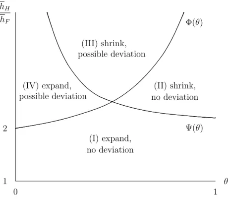
Ψ(θ)≡ (1− θ)D(L) D(θL)− θD(L) < hH hF ≤ 2− θ 1− θ ≡ Φ(θ). Proof. See Appendix G.
The condition for the variety loss can be rewritten as Ψ(θ) < hH/hF, whereas the sufficient
condition implies hH/hF ≤ Φ(θ). There are four possible cases, depending on whether or not (16)
and (19) are satisfied. Case (I) in Figure 1 shows that when hH/hF is sufficiently small, no firm
wants to deviate, and hence, PPE and FPE hold. Furthermore, product diversity expands in both countries under free trade irrespective of the value of θ. More interestingly, in case (II), there exists couples (θ, hH/hF) such that no firm wants to deviate, and hence, PPE and FPE hold; whereas
product diversity in consumption shrinks in the higher income country when switching from autarky to trade. This may make consumers in the higher income country worse off, depending on the relative importance of product diversity and pro-competitive effects. In cases (III) and (IV), when
θ is small and hH/hF is large enough, the sufficient condition for no deviation is not satisfied and
hence PPE and FPE may not hold. Turning to the case of the exponential distribution, we can show the following result.
Insert Figure 1 about here.
Proposition 7 Assume that Gr(hr) = 1− e−λrhr for country r = H, F , where the mean of each
distribution is given by hr ≡ 1/λr. Then, the condition for the variety loss (16) and the sufficient
condition (19) jointly hold when the share of population in country H, θ, is sufficiently large and the relative average labor efficiency satisfies
hH
hF
> 2 +[α + cD(L)] f cL .
Proof. See Appendix H.
Note that this result for exponential distributions is consistent with that for point-mass distribu-tions illustrated as “(II) shrink, no deviation” in Figure 1. We will show below that our numerical illustrations are in accordance with these theoretical results.
5
Numerical illustration
How many individuals in the higher income country may lose from trade? The answer hinges on the distribution functions GH and GF. To illustrate the quantitative properties of our model, we now
compute the share of the U.S. population who lose from trade. In so doing, we first use exponential distributions for which we have obtained a sufficient condition in terms of primitives.17 We then check the robustness of our results by using non-parametric income distributions in Section 6.1. To get clear-cut results, we first analyze the case of hypothetical bilateral trade liberalization between the U.S. and each of 188 countries, using 2005 data. We then turn to the case of multilateral trade liberalization using the historical sequence of U.S. free trade agreements (FTAs) since 1985. A detailed data description and information on the numerical procedure are relegated to Appendix J.
5.1
Bilateral trade liberalization
We first illustrate the quantitative properties of our model in the case of bilateral trade liberalization. Figure 2 depicts the relationship between the percentage of the U.S. population who lose from trade and real GDP per capita of the trading partners for the case of exponential distributions. The threshold GDP per capita of the trading partner below which we observe losses from trade for some U.S. consumers is about $18,000. U.S. intra-industry trade with countries of similar GDP per capita makes all individuals better off because it reduces the price-wage ratios and expands the range of varieties consumed in both countries, as shown in Propositions 2 and 3. However, U.S. trade with countries having lower GDP per capita may adversely affect up to 10% of the U.S. population.18 The
reason is that such trade reduces product diversity in consumption, although the price-wage ratios decrease. As argued before, less diversity hurts mainly the higher income consumers, whereas lower markups benefit mostly the lower income consumers.
17Exponential distributions are a special case of Gamma distributions analyzed in Salem and Mount (1974), and
provide reasonable approximations of the U.S. income distribution (e.g., Dra˘gulescu and Yakovenko, 2001).
18The condition in Proposition 5 is only sufficient but not necessary for the symmetric price equilibrium. While the
sufficient condition is useful for illustrating theoretical results, in the numerical analysis we rely on the more stringent necessary and sufficient condition Πr(ep) ≤ Πr(p) for all ep ≥ p. Figure 2 plots all the 143 countries for which that
Insert Figure 2 and Table 1 about here.
As seen from the top half of Table 1, the average share of U.S. losers increases monotonically from about 0% to 9.66% as the average income of the trading partners decreases. Observe that 25 out of the 27 high income OECD trading partners lead to 0% of losers, whereas for the remaining 2 high income OECD countries (Hungary and Slovak Republic) the percentage of losers is almost zero. Hence, U.S. intra-industry trade with high income OECD countries is beneficial to almost all U.S. consumers. Yet, trade with the upper middle income OECD countries (Mexico, Poland, and Turkey) generates some losers with the percentage being between 0.23% and 1.96%.19
We have so far focused on the share of U.S. losers by assuming that the U.S. actually trades with each trading partner. Whether or not the U.S. as a whole is likely to agree on free trade with each potential trading partner is another interesting question. Needless to say, investigating that question requires an assumption on the relevant political process. Although such an analysis is beyond the scope of this paper, Table 1 shows that the share of potential losers is not overwhelming in all cases, thus suggesting that U.S. intra-industry trade, even with highly dissimilar countries, need not require protection.20
5.2
Multilateral trade liberalization
We next turn to multilateral trade to investigate how the historical sequence of U.S. FTAs, as summarized in Table 2, has affected the individual welfare of the U.S. population. To this end, we extend our model to a multi-country setting (see Appendix I, where we provide key expressions). We start by examining the impacts of the U.S. FTA with Israel in 1985. We then consider how the newly integrated economy is affected by the U.S. FTA with Canada in 1988; how the newly integrated economy is affected by the entry of Mexico in 1994; and so on. We repeat this process of
19As seen from Table 1, the necessary and sufficient condition for the symmetric price equilibrium is less likely to
hold when the trading partners are big and/or have low income. The average GDP per capita in countries satisfying that condition is about $15,000, whereas that in the other countries is only about $1,400. Also, the former countries are much smaller, with an average population of about 16 million against an average population of about 90 million.
20Consider, for example, a simple political process based on majority voting. Let bh
H stand for the median of the
distribution GH. Then, comparing hlossH and bhH, we see that free trade is the social outcome if and only if bhH < hlossH .
trade integration until 2009. At each step of the process, we analyze how U.S. varieties and markups change, and who benefits from those changes. However, there are usually several years between successive FTAs, so that the growth of the U.S. population and of average labor efficiency affect welfare even when there are no additional FTAs. We eliminate these ‘growth effects’, which are not directly linked to FTAs, in order to highlight the impacts of adding new trading partners per se on individual gains from trade.
Insert Table 2 about here.
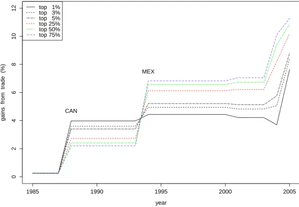
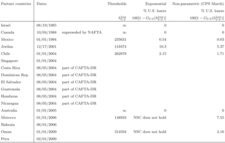
Figure 3 shows the successive changes in individual welfare for selected percentiles of the U.S. income distribution as compared to the base year 1985. Welfare changes in the sequence of U.S. FTAs need not be monotone, and it is the lower income consumers who eventually have gained more from these trade liberalizations. Observe that the 2001 FTA and the 2004 FTAs reduce the gains from trade at the top of the U.S. income distribution (the top 5% in the 2001 FTA, and the top 1% in the 2004 FTAs). Though the top 5% of agents still gain as compared to the initial situation in 1985, their gains would have been larger had either the 2001 or the 2004 FTAs not occurred. Observe further that the U.S. FTA with Canada (a country of similar income) in 1988 benefits mostly the richer consumers, whereas the U.S. FTA with Mexico (a country of lower income) in 1994 benefits mostly the lower income consumers. As can be seen from Table 2, which summarizes the different thresholds, hloss
U S, and the percentages of losers, 100[1− GU S(hlossU S)], for the different FTAs, trade with
Mexico even hurts the very upper end of the U.S. income distribution (less than the top 1%). Insert Figures 3 and 4 about here.
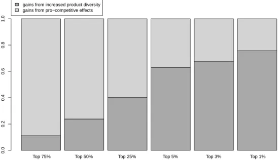
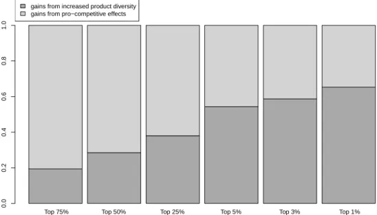
To illustrate our key mechanism, we decompose the welfare changes due to the FTA with Canada into product diversity and pro-competitive effects, as given by (18), for selected percentiles of the U.S. income distribution. Figure 4 shows that increased product diversity contributes 23.8% to the welfare change at the median income level, whereas the remaining 76.2% arises from increased consumption due to lower markups. The corresponding figures at the upper 5th percentile of the income distribu-tion are 63.0% for product diversity and 37.0% for pro-competitive effects, respectively. Clearly, the relative importance of product diversity increases with income.
6
Robustness
We now show that our main results are robust when using non-parametric income distributions and when extending the model to more than one sector.
6.1
Non-parametric income distributions
As a first robustness check, we run our numerical simulations using non-parametric income distri-butions. Doing so allows us to use more detailed information on the U.S. income distribution, and to check how sensitive our results are to the choice of that distribution.21 More precisely, we use
information on annual income for about 33,000–55,000 U.S. full-time earner households from the Current Population Survey (CPS) March Supplements between 1985 and 2009. See Appendix J for additional details on data and the numerical implementation.
6.1.1 Bilateral trade liberalization
We first consider bilateral trade liberalization in the non-parametric case using the same year 2005 and the same 188 trading partners as in Section 5.1. Figure 5 and Table 1 show that our results are robust. In particular, Table 1 shows that the average share of losers in the U.S. increases monotonically as the average income of the trading partners decreases. The shares of losers under the non-parametric distribution tend to be smaller than the corresponding shares under the exponential distribution when considering trade with low income countries, whereas the reverse holds for trade with high income countries. Yet, the correlation between the shares of losers in the exponential case and those in the non-parametric case exceeds 0.98. When focusing on the trading partners that generate U.S. losers, the average share of losers in the U.S. is 4.77% in the exponential case, while that in the non-parametric case is 3.03%.
Insert Figures 5–7 about here.
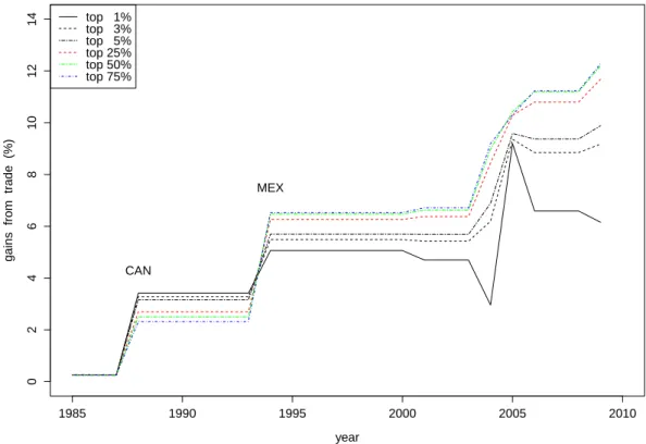
6.1.2 Multilateral trade liberalization
We next consider multilateral trade liberalization using the historical sequence of U.S. FTAs and the CPS household income distribution in each year. Figures 6 and 7 show that our qualitative and quantitative results are almost unchanged. In particular, the entry of Canada in 1988 (resp., Mexico in 1994) benefits mostly the higher (resp., lower) income consumers in the U.S. The entry of Mexico reduces the mass of varieties consumed, so that the richer consumers in the U.S. lose from trade integration with Mexico.22 This is not visible from Figure 6 since the income level of the losers is beyond the 1st percentile of the income distribution, as reported in Table 2. The overall conclusion that the lower income consumers gain more between 1985 and 2009 remains unchanged.23
6.2
Multiple sectors
One may argue that our single-sector results do not hold in a setting with multiple sectors as con-sumers who lose from less varieties in one sector may still gain because they benefit from lower markups in other sectors. We now show that this need not be the case. More precisely, some consumers may still lose overall, even though they gain in other sectors.
6.2.1 Model
To see this, we embed income heterogeneity in the two-sector model of Behrens and Murata (2012). Denoting the two sectors by 1 and 2, the problem of a consumer with income Er(hr) is given by:
max Ur ≡ U(U1r, U2r) s.t. ∫ Ω1r p1r(i)q1r(i)di + ∫ Ω2r p2r(j)q2r(j)dj = Er(hr), with U1r ≡ ∫ Ω1r[1− e
−α1q1r(i)]di and U
2r ≡
∫
Ω2r[1− e
−α2q2r(j)]dj. Assume, without loss of generality,
that α1 > α2. We can derive the demands as follows:
q1r(i, hr) = 1 α1 ln [ ρ1r(hr) p1r(i) ] and q2r(j, hr) = 1 α2 ln [ ρ2r(hr) p2r(j) ] , (20)
22The same results hold for the Gamma and Lognormal distributions (available upon request).
23Contrary to the exponential case, the necessary and sufficient condition in Appendix J holds for all years in the
where the reservation prices ρ1r(hr) and ρ2r(hr) are different across consumers but common to all
firms in the same industry. The expressions of the reservation prices are as follows: ρ1r(hr) ≡ e
α1Er(hr)
Pr +HrPr−α2Prα1 ln
(
α2
α1∂Ur /∂U2r∂Ur /∂U1r
) ∫ Ω2rp2r(j)dj (21) ρ2r(hr) ≡ e α1Er(hr) Pr +HrPr+Pr1 ln (α2 α1 ∂Ur /∂U2r ∂Ur /∂U1r ) ∫ Ω1rp1r(i)di , (22) where Pr ≡ ∫ Ω1rp1r(i)di + (α1/α2) ∫
Ω2rp2r(j)dj is the sum of prices and Hr ≡
∫
Ω1rp1r(i) ln p1r(i)di
+(α1/α2)
∫
Ω2rp2r(j) ln p2r(j)dj is a measure of price dispersion in the two-sector economy.
Assume that each firm serves all consumers in both countries under free trade (see Appendix J for the necessary and sufficient condition). The aggregate demand for variety i of sector 1 produced in country r is given by:
Q1r(i) = Lr ∫ q1r(i, hr)dGr(hr) + Ls ∫ q1s(i, hs)dGs(hs) = Lr α1 ∫ ln [ ρ1r(hr) p1r(i) ] dGr(hr) + Ls α1 ∫ ln [ ρ1s(hs) p1r(i) ] dGs(hs) = Lr+ Ls α1 [κ1− ln(p1r(i))] , where κ1 ≡ ∫ ln(ρ1r(hr))dGr(hr) + ∫
ln(ρ1s(hs))dGs(hs). Since κ1 is taken as given by each firm,
the own-price derivative is equal to −(Lr + Ls)/(α1p1r(i)). Each firm maximizes profits, and the
first-order condition is given by:
∂Π1r(i) ∂p1r(i) = Lr+ Ls α1 [ κ1− ln(p1r(i))− p1r(i)− cwr p1r(i) ] = 0. (23)
Solving condition (23), we then get the profit-maximizing price as follows:
p1r(i) = cwr W1r , with W1r = W ( ecwr eκ1 ) , (24)
where W denotes the Lambert W function (see Behrens and Murata, 2012). Mirror expressions hold for sector 2. In what follows, we thus only give expressions for sector 1. Expression (24) shows that the price equilibrium within each sector in each country is symmetric, since κ1 and marginal cost
cwr are common to all firms within the same sector in the same country.
Plugging the profit-maximizing price (24) into the first-order condition (23), we get Q1r(i) =
[(Lr+ Ls)/α1] [1− W1r], which then implies that
Π1r(i) = (Lr+ Ls)cwr α1 [ 1 W1r + W1r− 2 ] − fwr.
We then can easily solve the zero profit condition for W1r as follows: W1r = 1− √ 4α1cf (Lr+ Ls) + (α1f )2− α1f 2c(Lr+ Ls) .
As can be seen from the foregoing expression, W1r = W1s = W1, so that wr = ws = w and
p1r = p1s = p1 from (24). In words, PPE and FPE hold.
To solve for the equilibrium, we have to specify the upper-tier utility Ur. Assume that Ur ≡
β1ln U1r + β2ln U2r, with β1, β2 > 0 and β1 + β2 = 1. Let γr(hr) denote the budget share of a
consumer with labor efficiency hr, allocated to the consumption of good 1. Let also N1 ≡ n1r + n1s
and N2 ≡ n2r + n2s denote the masses of varieties in sectors 1 and 2, respectively. As the price
equilibrium is symmetric within each sector, we then have q1r(hr) = γr(hr)whr/(N1p1) and q2r(hr) =
(1− γr(hr))whr/(N2p2). Labor market clearing in country r requires that
Lrhr = ν1 [ W1Lr ∫ γr(hr)hrdGr(hr) + W1Ls ∫ γs(hs)hsdGs(hs) + N1f ] (25) +ν2 [ W2Lr ∫ (1− γr(hr))hrdGr(hr) + W2Ls ∫ (1− γs(hs))hsdGs(hs) + N2f ] ,
where we have used the price equilibrium (24), and where ν1 ≡ n1r/N1 and ν2 ≡ n2r/N2 denote the
share of sector 1 firms and that of sector 2 firms in country r.
Using the same notation as above, the trade balance condition is given by:
Lr [ (1− ν1) ∫ γr(hr)hrdGr(hr) + (1− ν2) ∫ (1− γr(hr))hrdGr(hr) ] = Ls [ ν1 ∫ γs(hs)hsdGs(hs) + ν2 ∫ (1− γs(hs))hsdGs(hs) ] . (26) Market clearing for good 1 can also be written in terms of γr(hr) and γs(hs) as follows:
LrW1 N1c ∫ γr(hr)hrdGr(hr) + LsW1 N1c ∫ γs(hs)hsdGs(hs) = Lr+ Ls α1 (1− W1). (27)
Finally, using the definition of γr(hr), as well as the expression of (∂Ur/∂U2r)/(∂Ur/∂U1r), demand
q1r(hr) for a consumer with labor efficiency hr can be rewritten as
γr(hr)whr N1p1 = whr P − 1 α1 ln p1+ H α1P − N2p2 α2P ln α2β2 α1β1 N1 [ 1− e−α1γr (hr )whrN1p1 ] N2 [ 1− e−α2(1−γr(hr))whrN2p2 ] . (28)
The general equilibrium of the two-sector model is given by the labor market clearing condition (25) for both countries r and s; by the trade balance condition (26); by the good market clearing
condition (27); and by the consumers’ cross-sector expenditure allocation conditions (28). Note that the last condition must hold for all hr in country r and all hs in country s. Put differently, we have
to solve for the four variables ν1, ν2, N1 and N2, as well as the two distributions γr(hr) and γs(hs).
Solving for the latter two when Gr and Gs are continuous is not analytically feasible and poses
numerical problems due to a continuum of equilibrium conditions. We hence discretize the model by replacing the integral expressions by discrete summations, and simulate it on discretized income distributions for both the U.S. and its trading partners. To make our results comparable to those of the single sector case, we restrict ourselves to discretized exponential distributions.24 For each distribution, we compute all income percentiles. We then associate the population of each percentile with the average income computed from that percentile. This discretization allows us to simulate the model while keeping the average income in each country at its observed level. Let γr(hir) denote
the expenditure share on good 1 in country r for the ith income percentile. The general equilibrium then consists of 204 equations in 204 unknowns (ν1, ν2, N1, N2, {γr(hir)}i=1,...,100,{γs(hjs)}j=1,...,100).
Appendix J provides additional details on the numerical implementation of the multi-sector case.
6.2.2 Numerical illustration
We illustrate the multi-sector model using bilateral trade between the U.S. and Brazil in 2005. Our choice is motivated by the fact that this example displays various impacts of trade on individual welfare across the U.S. income distribution. Unlike in the single-sector case, we can now decompose gains from trade on a sector-by-sector basis. Depending on an individual’s position in the U.S. income distribution, s/he may: (i) gain in both sectors; (ii) gain in one sector, but lose in the other, with the overall welfare change being positive; (iii) gain in one sector, but lose in the other, with the overall welfare change being negative; or (iv) lose in both sectors. We will show when each case arises in our example.
As explained in Section 6.2.1, we discretize exponential income distributions for both the U.S. and Brazil at each percentile. Using those discretized distributions, we then compute the equilibrium under both free trade and autarky to evaluate the changes in varieties and markups in each sector. Finally, we can compute, for each income percentile, the welfare change in each sector as well as the
overall welfare change.
Insert Figure 8 about here.
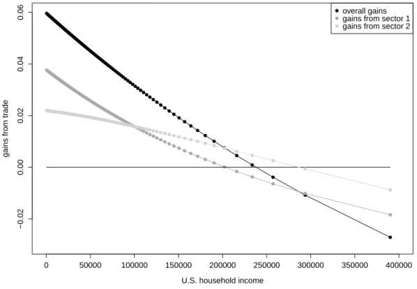
Figure 8, where each bullet corresponds to a percentile of the U.S. income distribution, displays the four cases explained above. First, for all consumers below the top 5% of the income distribution, gains from trade are positive in each sector. The reason is that, although consumption diversity shrinks, markups fall too, and the lower the income, the more important the price changes are for welfare as compared to the variety changes. Second, for all consumers between the top 4–5%, overall welfare gains are still positive. Although these consumers lose from reduced product diversity in sector 1 (the high α sector), gains in sector 2 due to lower markups more than compensate for the losses in sector 1. Third, for all consumers at the top 3%, overall welfare gains are negative, because losses from trade in sector 1 are not offset by gains in sector 2. Last, the top 1–2% consumers unambiguously lose from trade in both sectors as reduced diversity in each sector is not compensated by lower markups.
7
Concluding remarks
Globalization is widely believed to yield gains from trade at the aggregate level, yet produces winners and losers at the individual level. In this paper, we have analyzed the impact of globalization on individual gains from trade in a general equilibrium model of monopolistic competition featuring income heterogeneity between and within countries. We have shown that, although trade always reduces markups in both countries, its impact on product diversity in consumption depends on their relative position in the world income distribution. The range of varieties consumed in the lower income country always expands, while that in the higher income country may shrink. When the latter occurs, it is the richer consumers in the higher income country who may lose from trade because the relative importance of variety versus quantity increases with income. We have illustrated the quantitative properties of our model using data on GDP per capita and population, as well as on the U.S. income distribution. It turns out that U.S. bilateral trade with countries of similar GDP per capita makes all individuals in both countries better off, whereas trade with countries having lower GDP per capita may adversely affect up to 10% of the U.S. population. Interestingly, our analysis
of the sequence of U.S. FTAs further suggests that trade with Canada benefits mostly the richer consumers in the U.S., the entry of Mexico benefits mostly the lower income consumers in the U.S., and that it is the lower income consumers who eventually gain more from these trade liberalizations. To focus entirely on how globalization affects individual welfare through product diversity and pro-competitive effects, we have developed a highly stylized model. The following two points should therefore be kept in mind. First, our analysis abstracts from the role of factor endowments in determining individual welfare. However, when there is more than one factor, for instance, skilled and unskilled workers, factor proportions theory generally predicts that skilled workers in a skill abundant country gain from trade, whereas the unskilled in that country lose. Second, to restrict ourselves to the interaction of income heterogeneity and variable demand elasticities, we have forgone firm heterogeneity. Yet, trade liberalization shifts demand towards larger firms, which tend to employ more skilled people and pay higher wages. Our results suggest that the welfare changes driven by these within-industry reallocations and by Stolper-Samuelson effects may get weakened or even reversed when product diversity, pro-competitive effects, and income heterogeneity are jointly taken into account. Ultimately, trade may not generate as much inequality in individual welfare as predicted by firm heterogeneity and factor proportions theories. Introducing all of these elements into a single framework appears to be a daunting but promising extension in order to get a fuller picture of the impact of globalization on individual gains from trade.
Acknowledgements. We thank Robert King, Esteban Rossi-Hansberg, Giordano Mion, Gianmarco
Ot-taviano, an anonymous referee, and seminar participants at various institutions for helpful comments and
suggestions. Behrens is holder of the Canada Research Chair in Regional Impacts of Globalization.
Finan-cial support from the crc Program of the SoFinan-cial Sciences and Humanities Research Council (sshrc) of Canada is gratefully acknowledged. Behrens furthermore gratefully acknowledges financial support from
fqrsc Qu´ebec (Grant NP-127178) and the sshrc Standard Research Grants Program. Murata gratefully acknowledges financial support from Japan Society for the Promotion of Science (17730165). This research
was partially supported by the Ministry of Education, Culture, Sports, Science and Technology (mext, Japan), Grant-in-Aid for 21st century coe Program. The usual disclaimer applies.
References
[1] Arkolakis, C., S. Demidova, P. Klenow and A. Rodr´ıguez-Clare (2008) Endogenous variety and the gains from trade, American Economic Review 98, 444-450.
[2] Badinger, H. (2007) Has the EU’s Single Market Programme fostered competition? Testing for a decrease in mark-up ratios in EU industries, Oxford Bulletin of Economics and Statistics 69, 497-519.
[3] Baldwin, R.E. and R. Forslid (2010) Trade liberalization with heterogeneous firms, Review of
Develop-ment Economics 14, 161–176.
[4] Balistreri, E. (1997) The performance of the Heckscher-Ohlin-Vanek model in predicting endogenous policy forces at the individual level, Canadian Journal of Economics 30, 1-17.
[5] Behrens, K., G. Mion, Y. Murata and J. S¨udekum (2009) Trade, wages, and productivity, CEPR
Discussion Paper #7369.
[6] Behrens, K. and Y. Murata (2012) Trade, competition, and efficiency, forthcoming in Journal of
Inter-national Economics, doi:10.1016/j.jinteco.2011.11.005
[7] Behrens, K. and Y. Murata (2007) General equilibrium models of monopolistic competition: a new approach, Journal of Economic Theory 136, 776-787.
[8] Broda, C. and J. Romalis (2009) The welfare implications of rising price dispersion. Mimeographed, University of Chicago.
[9] Broda, C. and D. Weinstein (2006) Globalization and the gains from variety, Quarterly Journal of
Economics 121, 541-585.
[10] Dhaene, J., S. Vanduffel, M.J. Goovaerts, R. Kaas, Q. Tang, and D. Vyncke (2006) Risk measures and comonotonicity: A review, Stochastic Models 22, 573-606.
[11] Domowitz, I., R.G. Hubbard and B.C. Petersen (1988) Market structure and cyclical fluctuations in U.S. manufacturing, Review of Economics and Statistics 70, 55-66.
[12] Dra˘gulescu, A. and V.M. Yakovenko (2001) Evidence for the exponential distribution of income in the USA, The European Physical Journal B 20, 585-589.
[13] Epifani, P. and G.A. Gancia (2011) Trade, markup heterogeneity and misallocations, Journal of
Inter-national Economics 83, 1-13.
[14] Fajgelbaum, P., G.M. Grossman and E. Helpman (2011) Income distribution, product quality, and international trade, Journal of Political Economy 119, 721-765.
[15] Feenstra, R.C. (2004) Advanced International Trade: Theory and Evidence. Princeton, NJ: Princeton Univ. Press.