HAL Id: hal-01391745
https://hal.inria.fr/hal-01391745
Submitted on 3 Nov 2016
HAL is a multi-disciplinary open access
archive for the deposit and dissemination of
sci-entific research documents, whether they are
pub-lished or not. The documents may come from
L’archive ouverte pluridisciplinaire HAL, est
destinée au dépôt et à la diffusion de documents
scientifiques de niveau recherche, publiés ou non,
émanant des établissements d’enseignement et de
Introducing context-dependent and spatially-variant
viewing biases in saccadic models
Olivier Le Meur, Antoine Coutrot
To cite this version:
Olivier Le Meur, Antoine Coutrot. Introducing context-dependent and spatially-variant viewing biases
in saccadic models. Vision Research, Elsevier, 2016, 121, pp.72 - 84. �10.1016/j.visres.2016.01.005�.
�hal-01391745�
Introducing context-dependent and spatially-variant
viewing biases in saccadic models
Olivier Le Meura, Antoine Coutrotb
aIRISA University of Rennes 1, Campus Universitaire de Beaulieu, 35042 RENNES, France bCoMPLEX, University College London, United Kingdom
Abstract
Previous research showed the existence of systematic tendencies in viewing be-havior during scene exploration. For instance, saccades are known to follow a positively skewed, long-tailed distribution, and to be more frequently ini-tiated in the horizontal or vertical directions. In this study, we hypothesize that these viewing biases are not universal, but are modulated by the semantic visual category of the stimulus. We show that the joint distribution of sac-cade amplitudes and orientations significantly varies from one visual category to another. These joint distributions are in addition spatially variant within the scene frame. We demonstrate that a saliency model based on this better understanding of viewing behavioral biases and blind to any visual informa-tion outperforms well-established saliency models. We also propose a saccadic model that takes into account classical low-level features and spatially-variant and context-dependent viewing biases. This model outperforms state-of-the-art saliency models, and provides scanpaths in close agreement with human be-havior. The better description of viewing biases will not only improve current models of visual attention but could also influence many other applications such as the design of human-computer interfaces, patient diagnosis or image/video processing applications.
Keywords: viewing biases, visual scanpath, visual attention, saliency
1. Introduction
When looking at complex visual scenes, we perform in average 4 visual fix-ations per second. This dynamic exploration allows selecting the most relevant parts of the visual scene and bringing the high-resolution part of the retina, the fovea, onto them. To understand and predict which parts of the scene are
5
likely to attract the gaze of observers, vision scientists classically rely on two
IFully documented templates are available in the elsarticle package on CTAN. ∗O. Le Meur. Authors contributed equally to this work.
groups of gaze-guiding factors: low-level factors (bottom-up) and observers or task-related factors (top-down).
Saliency modeling: past and current strategies
10
A recent review of 63 saliency models from the literature showed that 47 of them use bottom-up factors, and only 23 use top-down factors (Borji & Itti, 2013). The great majority of these bottom-up models rely on the seminal con-tribution of (Koch & Ullman, 1985). In this study, the authors proposed a plausible computational architecture to compute a single topographic saliency
15
map from a set of feature maps processed in a massively parallel manner. The saliency map encodes the ability of an area to attract one’s gaze. Since the first models (Clark & Ferrier, 1988; Tsotsos et al., 1995; Itti et al., 1998), their performance has increased significantly, as shown by the on-line MIT bench-mark (Bylinskii et al., 2015). However, several studies have pointed out that,
20
in many contexts, top-down factors clearly take the precedence over bottom-up factors to explain gaze behavior (Tatler et al., 2011; Einh¨auser et al., 2008; Nystr¨om & Holmqvist, 2008). Several attempts have been made in the last several years to add top-down and high-level information in saliency models. (Torralba et al., 2006) improve the ability of bottom models by using global
25
scene context. (Cerf et al., 2008) combine low-level saliency map with face detection. (Judd et al., 2009) use horizon line, pedestrian and cars detection. (Le Meur, 2011) use two contextual priors (horizon line and dominant depth of the scene) to adapt the saliency map computation. (Coutrot & Guyader, 2014a) use auditory information to increase the saliency of speakers in
conver-30
sation scenes.
Saliency map representation is a convenient way to indicate where one is likely to look within a scene. Unfortunately, current saliency models do not make any assumption about the sequential and time-varying aspects of the overt atten-tion. In other words, current models implicitly make the hypothesis that eyes
35
are equally likely to move in any direction. Saccadic models introduced in the next section strive to overcome these limitations.
Tailoring saliency models to human viewing biases
Rather than computing a unique saliency map, saccadic models aim at
predict-40
ing the visual scanpaths, i.e. the suite of fixations and saccades an observer would perform to sample the visual environment. As saliency models, saccadic models have to predict the salient areas of our visual environment. But the great difference with saliency models is that saccadic models have to output plausible visual scanpaths, i.e. having the same peculiarities as human scanpaths. (Ellis
45
& Smith, 1985) pioneered in this field by elaborating a general framework for generating visual scanpaths. They used a stochastic process where the position of a fixation depends on the previous fixation, according to a first-order Markov process. This framework was then improved by considering saliency informa-tion, winner-take-all algorithm and inhibition-of-return scheme (Itti et al., 1998;
50
Itti & Koch, 2000). More recently, we have witnessed some significant achieve-ments thanks to the use of viewing behavioral biases, also called systematic
tendencies (Tatler & Vincent, 2009). The first bias that has been considered is related to the heavy-tailed distribution of saccade amplitudes. Saccades of small amplitudes are indeed far more numerous than long saccades. Small
sac-55
cades would reflect a focal processing of the scene whereas large saccades would be used to get contextual information. The latter mechanism is associated to ambient processing (Follet et al., 2011; Unema et al., 2005). A second bias concerns the distribution of saccade orientations. There is indeed an asymme-try in saccade orientation. Horizontal saccades (leftwards or rightwards) are
60
more frequent than vertical ones, which are much more frequent than oblique ones. (Foulsham et al., 2008) explain some of the possible reasons behind this asymmetry in saccade direction. First, this bias might be due to the dominance of the ocular muscles, which preferentially trigger horizontal shifts of the eyes. A second reason is related to the characteristics of natural scenes; this
encom-65
passes the importance of the horizon line and the fact that natural scenes are mainly composed by horizontally and vertically oriented contours. The third reason cited by (Foulsham et al., 2008) relates to how eye-tracking experiments are carried out. As images are most of the time displayed onscreen in landscape mode, horizontal saccades might be the optimal solution to efficiently scan the
70
scene.
The use of such oculomotor constraints allows us to improve the modelling of scanpaths. (Brockmann & Geisel, 2000) used a L´evy flight to simulate the scan-paths. This approach has also been followed in (Boccignone & Ferraro, 2004), where gaze shifts were modeled by using L´evy flights constrained by salience.
75
L´evy flight shifts follow a 2D Cauchy distribution, approximating the heavy-tailed distribution of saccade amplitudes. (Le Meur & Liu, 2015) use a joint distribution of saccade amplitudes and orientations in order to select the next fixation location. Rather than using a parametric distribution (e.g. Gamma law, mixture of Gaussians, 2D Cauchy distributions), (Le Meur & Liu, 2015)
80
use a non-parametric distribution inferred from eye tracking data.
In this paper, we aim at further characterizing the viewing tendencies one follows while exploring visual scenes onscreen. We hypothesize that these ten-dencies are not so systematic but rather vary with the visual semantic category
85
of the scene.
Visual exploration: a context-dependent process
Exploration of visual scenes has been tackled through two interdependent pro-cesses. The first one proposes that exploration is driven by the content, i.e.
influ-90
enced by low-level statistical structural differences between scene categories. It is well known that low-level features such as color, orientation, size, luminance, motion guide the deployment of attention (Wolfe & Horowitz, 2004). Many stud-ies have linked physical salience and eye movements within static (Parkhurst et al., 2002; Peters et al., 2005; Tatler et al., 2005), and dynamic natural
95
scenes (Carmi & Itti, 2006; Mital et al., 2010; Smith & Mital, 2013; Coutrot & Guyader, 2014b). Thus, scene categories could affect visual exploration through saliency-driven mechanisms, caused by systematic regularities in the distribution
of low-level features. For instance, city images usually have strong vertical and horizontal edges due to the presence of man-made structures (Vailaya et al.,
100
2001). The second process considers scene context as the relations between depicted objects and their respective locations within the scene. This global knowledge of scene layout provides observers with sets of expectations that can guide perception and influence the way they allocate their attention (Bar, 2004). These studies start from the observation that humans can recognize and
catego-105
rize visual scenes in a glance (Biederman et al., 1974), i.e. below 150 ms (Thorpe et al., 1996), or even below 13 ms (Potter et al., 2014). Bar proposed that this extremely rapid extraction of conceptual information is enabled by global shape information conveyed by low spatial frequencies (Bar, 2004). Each visual scene would be associated to a ‘context frame’, i.e. a prototypical representation of
110
unique contexts (Bar & Ullman, 1996). This contextual knowledge (learnt in-tentionally or incidentally through experience) helps us to determine where to look next (Henderson & Hollingworth, 1999; Chun, 2000). For instance, ob-jects of interest such as cars or pedestrians tend to appear in the lower half of the visual field in city street scenes. In a nutshell, the first glance establishes
115
the context frame of the scene, which then impacts the following exploration (see (Wu et al., 2014) for a review). The nature of the relative contributions of these two processes is still an open question. A recent study tried to dis-entangle the contributions of low-level features and knowledge of global scene organization (O’Connell & Walther, 2015). Participants either freely explored
120
the entire image (and thus made use of both physical salience and scene category information), or had their gaze restricted to a gaze-contingent moving window (peripheral access to the physical salience was blocked, encouraging the use of content-driven biases). The authors found distinct time courses for salience-driven and content-salience-driven contributions, but concluded that the time course of
125
gaze allocation during free exploration can only be explained by a combination of these two components.
So far, attention models have mostly relied on the first process, considering each low-level feature as an isolated factor able to attract attention by itself (with
130
the notable exception of Torralba’s Contextual Guidance model (Torralba et al., 2006)). In this paper, we propose a new framework binding low-level saliency with context-based viewing tendencies triggered by a swift recognition of scene category.
135
Contributions
As in (Tatler & Vincent, 2009), we believe that understanding and incorpo-rating viewing behavioral biases into saccadic models will help improve their performance. However, we think that these viewing biases are not universal, but are tuned by the semantic visual category of the stimulus. To test this
140
hypothesis, we use 6 eye tracking datasets featuring different categories of vi-sual content (static natural scenes, static web pages, dynamic landscapes and conversational videos). For each dataset, we compute the joint distribution of saccade amplitudes and orientations, and outline strong differences between
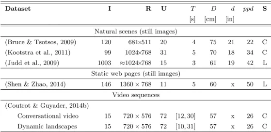
Dataset I R U T D d ppd S [s] [cm] [in]
Natural scenes (still images)
(Bruce & Tsotsos, 2009) 120 681×511 20 4 75 21 22 C (Kootstra et al., 2011) 99 1024×768 31 5 70 18 34 C (Judd et al., 2009) 1003 ≈1024×768 15 3 61 19 42 L
Static web pages (still images)
(Shen & Zhao, 2014) 146 1360 × 768 11 5 60 x 50 L Video sequences
(Coutrot & Guyader, 2014b)
Conversational video 15 720 × 576 72 [12, 30] 57 x 26 C Dynamic landscapes 15 720 × 576 72 [10, 31] 57 x 26 C
Table 1: Eye fixation datasets used in this study. (I is the number of images (or video se-quences), R is the resolution of the images, U is the number of observers, T is the viewing time, D is the viewing distance, d is the screen diagonal, ppd is the the number of pixel per visual de-gree, S=[C=CRT; L=LCD] is the screen type). x means that this information is not available. All stimuli and eye-tracking data are available online: http://www-sop.inria.fr/members/ Neil.Bruce/, http://www.csc.kth.se/~kootstra/index.php?item=215&menu=200, http:// people.csail.mit.edu/tjudd/WherePeopleLook/index.html, https://www.ece.nus.edu.sg/ stfpage/eleqiz/webpage_saliency.html and http://antoinecoutrot.magix.net/public/ databases.html, respectively.
them. We also demonstrate that these distributions depend on the spatial
lo-145
cation within the scene. We show that, for a given visual category, (Le Meur & Liu, 2015)’s saccadic model tuned with the corresponding joint distribution of saccade amplitudes and orientations but blind to low-level visual features significantly performs well to predict salient areas. Going even further, combin-ing our spatially-variant and context-dependent saccadic model with bottom-up
150
saliency maps allows us to outperform the best-in-class saliency models.
The paper is organized as follow. Section 2 presents on one hand the eye tracking datasets used in this study and on the other hand the method for esti-mating the joint distribution of saccade amplitudes and orientations. Section 3
155
demonstrates that the joint distribution of saccade amplitudes and orientations is spatially-variant and scene dependent. In Section 4, we also evaluate the ability of these viewing biases to predict eye positions as well as the perfor-mance of the proposed saccadic model. Section 5 discusses the results and some conclusions are drawn in Section 6.
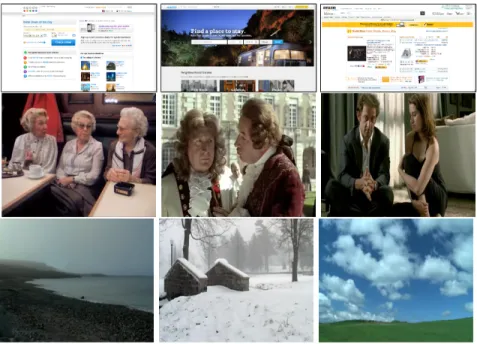
Figure 1: Sample images from (Shen & Zhao, 2014)’s datasets (Top row) and from (Coutrot & Guyader, 2014b) (Second row presents images from the face category whereas the third row presents images from the landscape category).
2. Method
2.1. Eye tracking datasets
Table 1 presents the six eye tracking datasets used in this study. They feature a large variety of visual content. (Bruce & Tsotsos, 2009; Kootstra et al., 2011; Judd et al., 2009)’s datasets are composed of natural static scenes. These first 3
165
datasets are classically used for benchmaking saliency models. (Shen & Zhao, 2014)’s dataset is composed of 146 static webpage images. The last dataset proposed by (Coutrot & Guyader, 2014b) is composed of video clips belonging to two different visual categories: humans having conversations, and landscapes. All the videos are shot with a static camera.
170
Figure 1 presents representative images of (Shen & Zhao, 2014) and (Coutrot & Guyader, 2014b)’s datasets.
2.2. Joint distribution of saccade amplitudes and orientations
When looking within complex scenes, human observers show a strong prefer-ence for making rather small saccades in the horizontal direction. Distribution of
175
saccade amplitudes is positively-skewed (Pelz & Canosa, 2001; Gajewski et al., 2005; Tatler & Vincent, 2008; Le Meur & Liu, 2015). As mentioned earlier, observers have also a strong bias to perform horizontal saccades compared to vertical ones.
To compute the joint probability distribution p(d, φ) of saccade amplitudes
180
and orientations, we follow (Le Meur & Liu, 2015)’s procedure. d and φ repre-sent the saccade amplitudes expressed in degree of visual angle and the angle between two successive saccades expressed in degree, respectively. Kernel den-sity estimation (Silverman (1986)) is used for estimating such a distribution. We define di and φi the distance and the angle between each pair of successive
185
fixations respectively. From all the samples (di, φi), we estimate the probability
that a fixation is featured by a distance d and an angle φ as follows:
p(d, φ) = 1 n n X i=1 Kh(d − di, φ − φi) (1)
where, n is the total number of samples and Khis a two-dimensional anisotropic
Gaussian kernel. h = (hd, hφ) is the kernel bandwidth. Separate bandwidths
were used for angle and distance components. We evenly divide the saccade
190
amplitude range into 80 bins (one bin representing 0.25◦) assuming that the maximum saccade amplitude is equal to 20◦. The angle φ ranges from 0 to 359◦ with a bin equal to one degree.
Rather than computing a unique joint distribution per image, we evenly di-vide the image into a N × N equal base frames. This process is illustrated in
195
Figure 2 for N = 3. N = 3 is a good trade-off between complexity and quality of the estimated distribution. Indeed it would not be appropriate to increase N because of the small number of saccades that would fall within base frames located on the borders. Decreasing N , i.e. N = 2, would spread the central saccades, which are the most numerous due to the center bias (Le Meur et al.,
200
2006; Tatler, 2007), over the 4 base frames. The numbering of base frames is given at the top-left corner of each base frame, as illustrated in Figure 2. The distributions of saccade orientations (shown on polar plot) which are superim-posed on the image are also showed. We will comment these distributions in Section 3.
205
3. Is the distribution of saccade amplitudes and orientations spatially-variant and scene dependent?
The joint distributions of saccade amplitudes and orientations are sepa-rately estimated for natural static scenes (images of Judd, Bruce and Kootstra’s datasets), static webpages (Shen’s dataset), conversational video sequences
in-210
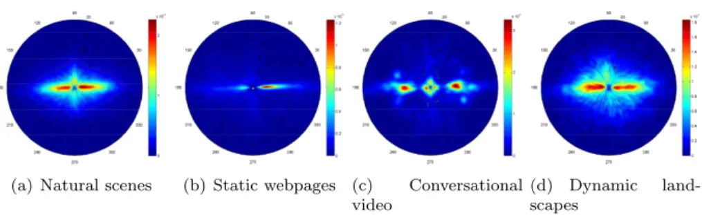
volving at least two characters (Coutrot’s dataset) and dynamic landscapes (Coutrot’s dataset). The subsequent analyses are performed over 87502, 27547, 41040 and 31000 fixations for the aforementioned categories, respectively. Fig-ure 3 shows the spatial dispersal of these fixations over the 3 × 3 grid. As expected, the image center plays an important role. This is especially
notice-215
able for the natural scenes (Figure 3 (a)) and the dynamic landscapes (Figure 3 (d)). For the webpages and conversational video sequences, the center bias is less important. Fixations are spread over the upper left-hand side for webpages whereas the upper part gathers most of the fixations for conversational video
Figure 2: Original image, extracted from (Coutrot & Guyader, 2014b)’s dataset, divided into 9 equal base frames. The distributions of saccade orientations are computed over each base frame. They are shown on polar plot and superimposed on the image.
sequences. These first results highlight that the content of scenes influences
220
visual behavior during task-free visual exploration.
In the following subsection, we analyze the joint distribution of saccade amplitudes and orientations for the different visual scenes. We also examine whether the joint distribution is spatially-invariant or not.
3.1. Influence of contextual information on saccade distribution
225
Figure 4 presents the joint distribution of saccade amplitudes and orienta-tions when we consider all fixaorienta-tions, i.e. N = 1. As expected, distribuorienta-tions are highly anisotropic. Saccades in horizontal directions are more numerous and larger than vertical ones. The distributions for natural scenes and dynamic landscapes share similar characteristics such as the horizontal bias (rightward
230
as well as leftward) and the tendency to perform vertical saccades in an upward directions. For webpages and conversational videos, we observe very specific distributions. The horizontal bias is present but mainly in the rightward direc-tion for webpages. This tendency is known as the F-bias (Buscher et al., 2009). Observers often scan webpages in a F-shaped pattern (raster scan order). For
235
conversational videos, the distribution also has a very specific shape. Before going further, let us recall that the conversational video sequences involve at least two characters who are conversing. Note, as well, that there is no camera motion. We observe three modes in the distribution (Figure 4 (c)): the first mode is located at the center and its shape is almost isotropic. Saccades are
(a) Natural scenes (b) Static webpages (c) Conversational video
(d) Dynamic land-scapes
Figure 3: Spatial spreading of visual fixations when images are split into 9 base frames as illustrated in Figure 2. The color scale expresses the percentage of visual fixations.
(a) Natural scenes (b) Static webpages (c) Conversational video
(d) Dynamic land-scapes
Figure 4: Joint distribution shown on polar plot for (a) Natural scenes, (b) Webpages, (c) conversational video and (d) dynamic landscapes.
rather small, less than 3 degrees. A plausible explanation is that the saccades of this mode fall within the face of one character. Observers would make short saccades in order to explore the face. Then the attention can move towards an-other character who could be located on the left or right-hand side of the current character. This could explain the two other modes of the distribution. These
245
two modes are elongated over the horizontal axis and gather saccades having amplitude in the range of 5 to 10 degrees of visual angle. As there is a strong tendency to make horizontal saccades, it could suggest that the characters’ faces are at the same level (which is indeed the case).
A two-sample two-dimensional Kolmogorov-Smirnov (Peacock, 1983) is
per-250
formed to test whether there is a statistically significant difference between the distributions illustrated in Figure 4. For two given distributions, we draw 5000 samples and test whether both data sets are drawn from the same distribution. For all conditions, the difference is significant, i.e. p << 0.001.
These results clearly indicate that the visual strategy to scan visual scene
255
is influenced by the scene content. The shape of the distribution of saccade amplitudes and orientations not only might be a relevant indicator to guess the type of scene an observer is looking at, but also a key factor to improve models of eye guidance.
1
2
3
4
5
6
7
8
9
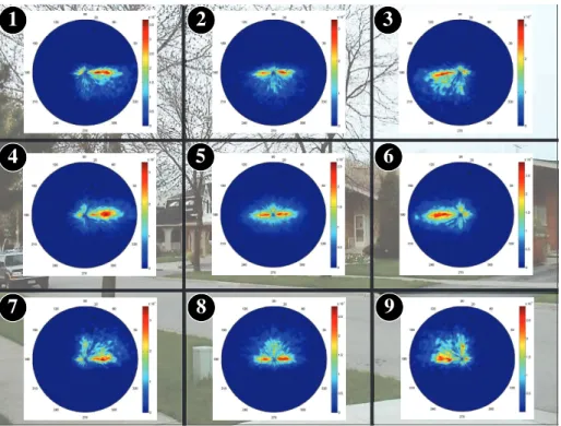
Figure 5: Probability distribution of saccade amplitudes and orientations shown on a polar plot (Natural scenes from Judd, Bruce and Kootstra’s dataset). A sample image belonging to this category is used as background image.
3.2. Is saccade distribution spatially-invariant?
260
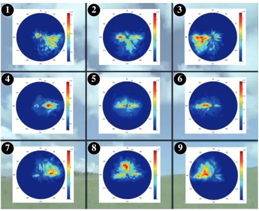
In this section, we investigate whether saccade distributions vary spatially or not. Figures 5, 6, 7 and 8 present the joint distributions of saccade amplitudes and orientations for the nine base frames spatially dividing the images and for the four categories, i.e. natural scenes, webpages, conversational video and dynamic landscapes.
265
Several conclusions can be drawn from these figures. First, whatever the considered datasets, the joint distributions dramatically vary from one base frame to another, and from one dataset to another.
For natural scenes and dynamic landscapes (see Figures 5 and 6), the well-known anisotropic shape of the joint distribution is observed in the fifth base
270
frame (the numbering is at the top-left corner of the base frames). For all other base frames, there is a strong tendency to make saccades towards the image’s center. The image edges repel the gaze toward the center. More specifically, we observe, for the base frames located at the image’s corners, i.e. numbered 1, 3, 7, and 9, rather large saccades in the diagonal direction (right,
down-275
left, up-right and up-left diagonal, respectively). This is also illustrated in Figure 2 for a conversational video sequence. For the base frames 2 and 8,
horizontal saccades (in both directions) and vertical saccades (downward and upward, respectively) are observed. Base frames 4 and 6 are mainly composed of rightward and leftward horizontal saccades, respectively. These saccades allow
280
us to refocus our gaze toward the image’s center.
Regarding webpages (see Figure 7), the saccades are mainly performed right-ward with rather small amplitudes. For the base frames numbered 3, 6 and 9, there are few but large diagonal and vertical saccades. This oculomotor behav-ior reflects the way we scan webpages. Observers explore the webpages from
285
the upper left corner in a pattern that looks like the letter F (Buscher et al., 2009). Eyes are re-positioned on the left-hand side of the webpage through large saccades in the leftward direction which are slightly tilted down, as illustrated by base frames 3 and 6.
For conversational video sequences (see Figure 8), a new type of distribution
290
shapes is observed. The distribution of the central base frame is featured by two main modes elongated over the horizontal axis and centered between 5 and 10 degrees of visual angle. As explained in the previous subsection, these two modes represent the faces of the conversation partners. Observers focus alternately their attention on one particular face. This behavior is also reflected
295
by the distributions shown in base frames 1, 2, 3, 4 and 6. They are composed of saccades with rather large amplitudes which are likely used to re-allocate the visual attention on the distant character. For instance, in base frame 4, the distribution mainly consists of rightward saccades. Concerning base frames 7, 8, and 9, the number of saccades is much lower. Saccades are oriented upward
300
in the direction of image’s center.
In conclusion, these results give new insights into viewing behavioral biases. Saccades distributions are not only scene-dependent but also spatially-variant.
4. Performance of the proposed saccadic model
In this section, we investigate whether the spatially-variant and scene
depen-305
dent viewing biases could be used to improve the performance of the saccadic model proposed in (Le Meur & Liu, 2015).
4.1. Gauging the effectiveness of viewing biases to predict where we look at As in (Tatler & Vincent, 2009), we evaluate first the ability of viewing biases to predict where we look at. We consider N = 3 base frames and the four joint
310
distributions computed from natural scenes, dynamic landscapes, conversational and webpages.
We modify the saccadic model proposed in (Le Meur & Liu, 2015) by con-sidering a uniform saliency map as input. It means that we know nothing about the scene. Another modification consists in using 9 distributions as illustrated
315
in the previous sections, instead of a unique and global joint distribution of sac-cade amplitudes and orientations. In this model, a parameter called Nc is used
to tune the randomness of the model: Nc = 1 leads to the maximum
1
2
3
4
5
6
7
8
9
Figure 6: Probability distribution of saccade amplitudes and orientations shown on a polar plot (dynamic landscapes from Coutrot’s dataset). A sample image belonging to this category is used as background image.
In this study, we keep the value recommended by (Le Meur & Liu, 2015), i.e.
320
Nc = 5. We generate 100 scanpaths, each composed of 10 fixations. The first
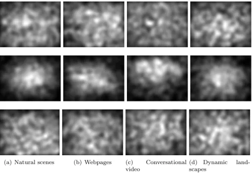
fixation point is randomly drawn. From the set of scanpaths, we generate pre-dicted saliency maps by convolving the fixation maps, gathering all prepre-dicted fixations, with a 2D Gaussian function, as described in (Le Meur & Baccino, 2013). Figure 9 presents the predicted saliency maps obtained by considering
325
viewing biases alone. We refer to these maps as viewing biases-based predicted saliency maps. The top row presents the saliency maps when considering that the joint distribution is spatially-invariant (i.e. N = 1). The distributions shown in Figure 4 are here used. The middle row of Figure 9 illustrates the predicted saliency maps when the distributions are considered as being spatially-variant.
330
In this case, nine distributions per category are used to get the map. In the bottom row of Figure 9, we wanted to demonstrate the importance of using the right distribution from the right base frame. For this purpose, the base frame numbering is shuffled before computing the predicted saliency maps. For instance, when a fixation falls within the base frame numbered one, instead of
1 2 3
4 5 6
7 8 9
Figure 7: Probability distribution of saccade amplitudes and orientations shown on a polar plot (Webpages from Shen’s dataset). A sample image belonging to this category is used as background image.
using the actual distribution of saccade amplitudes and orientations, we use the distribution of the base frame numbered 9 to predict the next fixation point.
When the viewing biases are described by only one distribution, viewing biases-based predicted saliency maps tend to be rather uniform, whatever the scene category (see top row of Figure 9). The similarity between predicted
340
saliency maps is qualitatively high although that the distributions we use are statistically different, as described in subsection 3.1. When we consider more than one distribution, i.e. 9, predicted saliency maps are less similar (middle row of Figure 9). The predicted salience associated to conversational videos is mainly located in the upper part of the scene, which is consistent with the
345
scene content. It is also noticeable that viewing biases-based predicted saliency maps (a), (b) and (d) corresponding to natural scenes, webpages and dynamic landscapes, respectively, are center-biased. This is due to the re-positioning saccades starting from the base frames located on the scene borders and landing around the center. When the base frame numbering is shuffled, the saliency
350
maps do not exhibit special properties, as illustrated by the bottom row of Figure 9. Qualitatively speaking, they are similar to saliency maps of the top row.
To assess the predictive power of viewing biases taken alone, the viewing biases-based predicted saliency maps are compared to human saliency maps
355
estimated from the eye fixation dataset of (Bruce & Tsotsos, 2009). We addi-tionally compare human saliency maps to maps computed by saliency models. Viewing biases-based predicted saliency maps and saliency maps coming from
1
2
3
4
5
6
7
8
9
Figure 8: Probability distribution of saccade amplitudes and orientations shown on a polar plot (conversational video from Coutrot’s dataset) A sample image belonging to this category is used as background image.
computational saliency models rely on two radically different strategies. The former is only based on the viewing biases and is blind to visual information in
360
the scene. The latter is based on a perfect knowledge of the visual scene but assumes there is no constraint on how eye movements are performed.
The similarity between saliency maps is quantified by using the linear corre-lation coefficient (noted CC), Earth Mover’s Distance measure (noted EM D) and histogram intersection (noted SIM ). The linear correlation coefficient
365
evaluates the degree of linearity between the two sets. It varies between -1 and -1. The Earth Mover’s Distance, also called Wasserstein metric, mea-sures the distance between two probability distributions and evaluates the min-imum cost for turning one distribution into the other. EM D = 0 for identical distributions. SIM computes the intersection between histograms. It varies
370
between 0 and 1. SIM = 1 means the distributions are identical. These three methods are used for benchmarking saliency models (see the website http://saliency.mit.edu/index.html, (Judd et al., 2012)).
bi-(a) Natural scenes (b) Webpages (c) Conversational video
(d) Dynamic land-scapes
Figure 9: Predicted saliency maps when we consider only the viewing biases. Top row: a unique joint distribution of saccade amplitudes and orientations is used (N=1). Middle row: 9 distributions are used (N=3). Bottom row: 9 distributions are also used but the saliency map is generated by shuffling the base frame numbering (N=3 Shuffled). Different scenes categories are considered natural scenes (a), webpages (b), conversational video (c) and dynamic landscapes (d).
ases estimated from eye movements recorded on Natural Scenes, Webpages,
Con-375
versational videos and Landscape videos. Viewing biases are estimated within a unique distribution (N=1), 9 distributions (N=3), and 9 shuffled distributions (N=3 Shuffled). For the sake of clarity, only CC are reported, but the results are similar for SIM and EMD. There is a great benefit to consider spatially-variant viewing biases. Indeed, whatever the metrics and the scene category, the ability
380
to predict where human observers fixate is much better when 9 distributions are considered. For natural scenes, the CC gain is 0.16. When the base frame numbering is shuffled, the performance dramatically drops. We ran a two-way ANOVA (Fx× category, where Fx= {FN =1, FN =3, FN =Shuf f led}) on CC scores.
We found a significant of visual category (F(3,1428)=38.3, p < 0.001), and of
385
Fx (F(2,1428)=222.6, p < 0.001), and of their interactions (F(6,1428)=64.5,
p < 0.001). Bonferroni post-hoc comparisons showed that CC scores are higher for N = 3 than for N = 1 or N = Shuf f led (both p < 0.001). There were no differences between N = 1 and N = Shuf f led (p = 0.16). Simple main effect analysis showed that CC scores are higher for N = 3 than for N = 1
390
for Landscapes, Natural Scenes and Webpages (all p < 0.001), but there were no differences for Faces (p = 0.2). These results support the fact that the
Figure 10: Correlation Coefficients (CC) of saliency maps only based on viewing biases (i.e. blind to image information) over Bruce’s dataset. We compare saliency maps composed of a unique distribution (N=1), 9 distributions (N=3), and 9 shuffled distributions (N=3 Shuf-fled). Saliency maps’ performances are compared when viewing biases are estimated from eye movements recorded on Natural Scenes, Webpages, Conversational videos and Dynamic Landscapes. Error bars denote ±1 standard deviations.
distribution of saccade is spatially-variant.
Table 2 compares saliency maps computed by state-of-the-art saliency mod-els with the context-independent saccadic model based on a single distribution
395
(N=1) from (Le Meur & Liu, 2015) and our context-dependent, spatially-variant saccadic model. First, by comparing Figure 10 with the upper part of Table 2, we observe that a computational model based on viewing biases alone signifi-cantly outperforms 3 out of the 7 tested saliency models. We ran a one-way ANOVA on CC scores1, and found a main effect of models (F(7,952)=49.05,
400
p < 0.001). Bonferroni post-hoc comparisons showed that CC scores are higher for N = 3 than for the models of Bruce, Itti and Le Meur (all p < 0.001). We found no differences between N = 3 and Garcia, (p = 0.31), Judd (p = 0.22) and Riche (p = 0.10) models. The only saliency model presenting higher CC scores is Harel’s model (p = 0.002). Regarding SIM scores, we found a main
405
effect of models (F(7,952)=53.3, p < 0.001). Bonferroni post-hoc comparisons showed that SIM scores are higher for N = 3 than for the models of Bruce, Itti and Judd (all p < 0.001). We found no differences between N = 3 and Garcia (p = 0.15) and Le Meur (p = 0.41). Harel and Riche models presented higher SIM scores than N = 3 (p = 0.02 and p = 0.002, respectively).
Fi-410
nally, we ran a one-way ANOVA on EMD scores, and found a main effect of models (F(7,952)=34.6, p < 0.001). Bonferroni post-hoc comparisons showed that EMD scores are lower for N = 3 than for Garcia, Bruce, Itti, Judd (all
1we consider the distributions computed from natural scenes since Bruce’s dataset is mainly
Metric CC SIM EMD
(B)
Bottom-up
features
alone
State-of-the-art saliency models
(Itti et al., 1998) 0.27±0.18 0.37±0.05 3.41±0.65 (Le Meur et al., 2006) 0.38±0.20 0.43±0.09 3.03±1.06 (Harel et al., 2006) 0.56±0.14 0.48±0.05 2.49±0.53 (Bruce & Tsotsos, 2009) 0.31±0.10 0.37±0.04 3.44±0.56 (Judd et al., 2009) 0.42±0.13 0.40±0.04 3.25±0.57 (Garcia-Diaz et al., 2012) 0.42±0.18 0.43±0.06 3.30±0.76 (Riche et al., 2013) 0.54±0.18 0.48±0.06 2.61±0.71 Top 2 models combined: (Riche et al., 2013) + (Harel et al., 2006) Top2(R+H) 0.62±0.13 0.514±0.05 2.282±0.56
Com
bining
(V)
and
(B) Saccadic saliency model (Top2(R+H)) context-independent, N = 1 (Le Meur & Liu, 2015) 0.641±0.18 0.568±0.09 2.03±0.85 Saccadic saliency model (Top2(R+H)) context-dependent, N = 3 Natural scenes 0.649±0.18 0.566±0.09 2.068±0.84 Webpages 0.641±0.18 0.561±0.09 2.177±0.88 Conversational 0.628±0.17 0.561±0.09 2.061±0.84 Landscapes 0.653±0.17 0.571±0.08 2.034±0.85
Table 2: Performance (average ± standard deviation) of saliency models over Bruce’s dataset. In pink cells, we compare state-of-the-art saliency maps with human saliency maps. We add the top 2 models ((Riche et al., 2013) + (Harel et al., 2006)) into a single bottom-up model: Top2(R+H). In green cells, we compare the performances when low-level visual features from Top2(R+H) and viewing biases are combined. First, we assess the context-independent saccadic model based on a single distribution (N=1) from (Le Meur & Liu, 2015). Second, we assess our context-dependent saccadic model based on 9 distributions (N=3), with viewing biases estimated from 4 categories (Natural Scenes, Webpages, Conversational videos and Landscape videos). Three metrics are used: CC (linear correlation), SIM (histogram similarity) and EMD (Earth Mover’s Distance). For more details please refer to the text.
p < 0.001) and Le Meur (p = 0.005) models. We found no differences between N = 3, Harel and Riche (all p = 1) models.
415
It is worth pointing out that, when the viewing biases used to estimate the predicted saliency maps do not correspond well with the type of the processed images, the performances decrease. This is illustrated by the conversational predicted saliency map, (see Figure 9 (c)), which does not perform well in pre-dicting human saliency. This is probably related to the fact that Bruce’s dataset
420
is mainly composed by natural indoor and outdoor scenes. In this context, the very specific conversational saliency map in which the salience is concentrated in the upper part turns out to be a poor saliency predictor.
category could be efficiently used to predict where observers look. This
signifi-425
cant role in guiding spatial attention could be further improved by considering the bottom-up salience. We investigate this point in the next section.
4.2. Bottom-up salience and viewing biases for predicting visual scanpaths Rather than considering a uniform saliency map as input of (Le Meur & Liu, 2015)’s model, as we did in the previous section, we use a saliency map
430
which is the average of the saliency maps computed by two well-known saliency models, namely (Harel et al., 2006) and (Riche et al., 2013). Combining (Harel et al., 2006) and (Riche et al., 2013) models (called Top2(R+H) in Table 2) sig-nificantly increases the performance, compared to the best performing saliency model, i.e. (Riche et al., 2013)’s model (see (Le Meur & Liu, 2014) for more
435
details on saliency aggregation). When the Top2(R+H) saliency maps are used as input of (Le Meur & Liu, 2015)’s model, the capacity to predict salient areas is getting higher than the Top2(R+H) model alone. For instance, there is a sig-nificant difference between the Top2(R+H) model and (Le Meur & Liu, 2015)’s model in term of linear correlation. The former performs at 0.62 whereas the
440
latter performs at 0.64 (paired t-test, p = 0.012), see Table 2.
When we replace invariant and context-independent joint distribution of sac-cade amplitudes and orientations used by (Le Meur & Liu, 2015) with spatially-variant and context-dependent joint distributions, the ability to predict where we look is getting better according to the linear correlation coefficient, with
445
the notable exception of conversational distribution. The best model is the model that takes into account the joint distribution computed from Landscapes datasets. Compared to (Le Meur & Liu, 2015)’s model, the linear correlation gain is 0.012, but without being statistically significant. The model using the joint distribution of natural scenes is ranked 2. We observe a loss of performance
450
when the joint distribution computed over conversational frames is used. Com-pared to (Le Meur & Liu, 2015)’s model, the linear correlation drops down from 0.641 to 0.628. According to SIM and EMD, the use of context-dependent and spatially-variant distributions does not further improve the ability to predict saliency areas.
455
From these results, we can draw some conclusions. Taken alone, the per-formance in term of linear correlation is, at most, 0.62 and 0.48 for bottom-up saliency map and viewing biases, respectively. As expected, the perfor-mance significantly increases when bottom-up saliency map are jointly con-sidered with viewing biases, with a peak of CC at 0.653. A similar trend is
460
observed for SIM and EMD metrics. However, we notice that the use of context-dependent and spatially-variant distributions does not significantly improve the prediction of salient areas compared to a model that would use invariant and context-independent joint distribution of saccade amplitudes and orientations. This result is disappointing since, as shown in Section 4.1, context-dependent
465
and spatially-variant distributions alone significantly outperform invariant and context-independent distribution when predicting salient areas. A major differ-ence between these two kinds of distribution is the presdiffer-ence of re-positioning sac-cades in the spatially-variant distributions; these sacsac-cades allow us to re-position
(a) Natural scenes (b) Static webpages (c) Conversational video
(d) Dynamic land-scapes
Figure 11: Joint distribution of predicted scanpaths shown on polar plot for (a) Natural scenes, (b) Webpages, (c) conversational video and (d) dynamic landscapes. Scanpaths are generated by the context-dependent saccadic saliency model (Top2(R+H), N = 3).
the gaze around the screen’s center, promoting the center bias. When
context-470
dependent and spatially-variant distributions are jointly used with bottom-up saliency maps, this advantage vanishes. There are at least two reasons that could explain this observation. The first one is that saliency models, such as Harel’s model (Harel et al., 2006), tend to promote higher saliency values in the center of the image. Therefore, the influence of re-positioning saccades on the
475
final result is less important. The other reason is that the use of viewing biases is fundamental to provide plausible visual scanpaths (see section 4.3), and, to a lesser extent, to predict eye positions.
We believe however that a better fit of the joint distributions to Bruce’s images would further increase the performance of our model on this dataset.
480
Indeed, we previously observed that the performance worsens when the joint distribution does not fit the visual category of Bruce’s images, e.g. when we use the joint distribution computed from conversational videos. To support this claim, we perform a simple test. As Bruce’s dataset is mainly composed of street images (about 46%) and indoor scenes (about 36%), we select for each image of
485
this dataset the best performance obtained by our saccadic model when using either Landscapes or Natural scenes joint distributions. We do not consider the two other distributions, i.e. Webpages and Conversational, considering that they do not correspond at all to Bruce’s dataset. We observe that the performances further increase for CC and SSIM metrics (CC = 0.661, SIM = 0.575) and
490
stay constant for EMD metric (EM D = 2.1). This result suggests that an even better description of viewing biases would further increase performance of saliency models.
4.3. Joint distribution of saccade amplitudes and orientations of predicted scan-paths
495
As discussed in the previous section, the saliency maps computed from the predicted visual scanpaths turn out to be highly competitive in predicting salient areas. But saccadic models not only predict bottom-up saliency, they also pro-duce visual scanpaths in close agreement with human behavior. Figure 11 (a) to (d) illustrates the polar plots of the joint distributions of saccade amplitudes and
orientations of predicted scanpaths, when considering context-dependent distri-butions. As expected, we observe that the predicted visual scanpaths charac-teristics (i.e. saccade amplitudes and orientations) are context-dependent. For instance, when the joint distribution estimated from static webpages is used by the saccadic model to predict scanpaths, the proportion of rightward saccades
505
is much higher than leftward saccades and vertical saccades. For conversational videos, we observe two dominant modes located on the horizontal axis. These observations are consistent with those made in Section 2.2. We can indeed no-tice a strong similarity between the joint distribution of saccade amplitudes and orientations of human scanpaths, illustrated in Figure 4, and those of predicted
510
scanpaths.
Joint distributions of Figure 11 exhibit however few short saccades and few vertical saccades. These discrepancies are likely due to the design of the inhibition-of-return mechanism used in (Le Meur & Liu, 2015). In the latter model, the spatial inhibition-of-return effect declines as an isotropic Gaussian
515
function depending on the cue-target distance (Bennett & Pratt, 2001). Stan-dard deviation is set to 2◦. These discrepancies might be reduced by considering anisotropic exponential decay and by considering a better parameter fitting.
5. Discussion
In the absence of an explicit task, we have shown that the joint distribution
520
of saccade amplitudes and orientations is not only biased by the scene category but is also spatially-variant. These two findings may significantly influence the design of future saliency models which should combine low-level visual features, contextual information and viewing biases.
Although we are at the incipient stage of this new era, it is worth noticing
525
that some saliency or saccadic models already embed viewing biases to predict where human observers fixate. The most used is the central bias which favors the center of the image compared to its borders. This bias is currently introduced in computational modeling through ad hoc methods. In (Le Meur et al., 2006; Marat et al., 2013), the saliency map is simply multiplied by a 2D anisotropic
530
Gaussian function. Note that the standard deviations of the Gaussian function can be learned from a training set of images to boost the performance, as rec-ommended by (Bylinskii et al., 2015). Bruce’s model (Bruce & Tsotsos, 2009) favors the center by removing the image’s borders whereas Harel’s model (Harel et al., 2006) do so thanks to its graph-based architecture. Saccade distributions
535
are used by saccadic models (Tavakoli et al., 2013; Boccignone & Ferraro, 2011) and allow to improve the prediction of salient areas (Le Meur & Liu, 2015). (Tatler & Vincent, 2009) went even further and considered the viewing biases alone. Without any visual input from the processed scene, they proposed a model outperforming state-of-the-art low-level saliency models.
540
However, these approaches suffer from the fact that they consider saccade distributions as being systematic and spatially-invariant. In this study, we show that considering the context-dependent nature of saccade distributions allow to further improve saccadic models. This is consistent with the recent findings
presented in (O’Connell & Walther, 2015). Indeed, this study shows that scene
545
category directly influences spatial attention. Going further, we also demon-strate that saccade distributions are spatially-variant within the scene frame. By considering category-specific and spatially-variant viewing biases, we demon-strate, in the same vein as (Tatler & Vincent, 2009), that these viewing biases alone outperform several well-established computational models. This model,
550
aware of the scene category but blind to the visual information of the image being processed, is able to reproduce, for instance, the center bias. The latter is simply a consequence of the saccade distributions of the base frames located on the image border. As previously mentioned, these base frames are mainly composed of saccades pointing towards the image’s center.
555
Visual attention deployment is influenced, but up to a limited extent, by low-level visual factors. (Nystr¨om & Holmqvist, 2008) demonstrated that high-level factors can override low-high-level factors, even in a context of free-viewing. (Einh¨auser et al., 2008) demonstrated that semantic information, such as ob-jects, predict fixation locations better than low-level visual features. (Coutrot
560
& Guyader, 2014b) showed that, while watching dynamic conversions, conversa-tion partners’ faces clearly take the precedence over low-level static or dynamic features to explain observers’ eye positions. We also demonstrate that a straight-forward combination of bottom-up visual features and viewing biases allows to further improve the prediction of salient areas.
565
From these findings, a new saliency framework binding fast scene recogni-tion with category-specific spatially-variant viewing biases and low-level visual features could be defined.
We believe that there is a potential to go further in the estimation and description of viewing biases. First, we assumed that saccades are independent
570
events and are processed separately. This assumption is questionable. (Tatler & Vincent, 2008) showed for instance that saccades with small amplitude tend to be preceded by other small saccades. Regarding saccade orientation, they noticed a bias to make saccades either in the same direction as the previous saccade, or in the opposite direction. Compared to the first-order analysis we
575
perform in this study, it would make sense to consider second-order effects to get a better viewing biases description. In addition, as underlined by (Tatler & Vincent, 2009), a more comprehensive description could take into account saccade velocity, as well as the recent history of fixation points.
One important characteristic of visual scanpaths, but currently missing in
580
the proposed model, is fixation duration. (Trukenbrod & Engbert, 2014) re-cently proposed a new model to predict the duration of a visual fixation. The prediction is based on the mixed control theory encompassing the processing difficulty of a foveated item and the history of previous fixations. Integrating (Trukenbrod & Engbert, 2014)’s model into our saccadic model would improve
585
the plausibility of the proposed model. Moreover, estimating fixation durations will open new avenues in the computational modelling of visual scanpaths, such as the modelling of microsaccades occurring during fixation periods (Martinez-Conde et al., 2013).
From a more practical point of view, one could raise concerns about the
number and the spatial layout of base frames. In this study, we give compelling evidence that saliency maps based on viewing biases are much better when nine base frames are used, i.e. N = 3. Increasing the number of base frames would most likely improve the prediction of salient areas. However, a fine-grained grid would pose the problem of statistical representativeness of the estimated
595
distributions. Regarding the base frame layout, one may wonder whether we should use evenly distributed base frames or not and whether base frames should overlap or not.
Eye movement parameters are not only spatially variant and scene category specific, but some very recent work showed that they also differ at an individual
600
level. Individual traits such as gender, personality, identity and emotional state could be inferred from eye movements (Nummenmaa et al., 2009; Mercer Moss et al., 2012; Greene et al., 2012; Chuk et al., 2014; Borji et al., 2015; Kanan et al., 2015). For instance, (Mehoudar et al., 2014) showed that humans have idiosyncratic scanpaths while exploring faces, and that these scanning patterns
605
are highly stable across time. Such stable and unique scanning patterns may represent a specific behavioral signature. This suggests that viewing biases could be estimated at an individual level. One could imagine training a model with the eye movements of a given person, and tune a saccadic model according to its specific gaze profile. This approach could lead to a new generation of
610
saliency-based application, such as user-specific video compression algorithm.
6. Conclusion
Viewing biases are not so systematic. When freely viewing complex images, the joint distribution of saccade amplitudes and orientations turns out to be spatially-variant and dependent on scene category. We have shown that saliency
615
maps solely based on viewing biases, i.e. blind to any visual information, out-perform well-established saliency models. Going even further we show that the use of bottom-up saliency map and viewing biases improves saliency model per-formance. Moreover, the sequences of fixation produced by our saccadic model get closer to human gaze behavior.
620
Our contributions enable researchers to make a few more steps toward the understanding of the complexity and the modelling of our visual system. In a recent paper, (Bruce et al., 2015) present a high-level examination of persisting challenges in computational modelling of visual saliency. They dress a list of obstacles that remain in visual saliency modelling, and discuss the biological
625
plausibility of models. Saccadic models provide an efficient framework to cope with many challenges raised in this review, such as spatial bias, context and scene composition, as well as oculomotor constraints.
References
Bar, M. (2004). Visual objects in context. Nature Reviews Neuroscience, 5 ,
630
Bar, M., & Ullman, S. (1996). Spatial context in recognition. Perception, 25 , 343–352.
Bennett, P. J., & Pratt, J. (2001). The spatial distribution of inhibition of return:. Psychological Science, 12 , 76–80.
635
Biederman, I., Rabinowitz, J. C., Glass, A. L., & Stacy, E. W. (1974). On the information extracted from a glance at a scene. Journal of experimental psychology, 103 , 597.
Boccignone, G., & Ferraro, M. (2004). Modelling gaze shift as a constrained random walk. Physica A: Statistical Mechanics and its Applications, 331 , 207
640
– 218. doi:http://dx.doi.org/10.1016/j.physa.2003.09.011.
Boccignone, G., & Ferraro, M. (2011). Modelling eye-movement control via a constrained search approach. In EUVIP (pp. 235–240).
Borji, A., & Itti, L. (2013). State-of-the-art in visual attention modeling. IEEE Trans. on Pattern Analysis and Machine Intelligence, 35 , 185–207.
645
Borji, A., Lennartz, A., & Pomplun, M. (2015). What do eyes reveal about the mind?: Algorithmic inference of search targets from fixations. Neurocomput-ing, 149 , 788–799.
Brockmann, D., & Geisel, T. (2000). The ecology of gaze shifts. Neurocomput-ing, 32 , 643–650.
650
Bruce, N., & Tsotsos, J. (2009). Saliency, attention and visual search: an information theoretic approach. Journal of Vision, 9 , 1–24.
Bruce, N. D., Wloka, C., Frosst, N., Rahman, S., & Tsotsos, J. K. (2015). On computational modeling of visual saliency: Examining whats right, and whats left. Vision research, .
655
Buscher, G., Cutrell, E., & Morris, M. R. (2009). What do you see when you’re surfing? using eye tracking to predict salient regions of web pages. In Proceedings of CHI 2009 . Association for Computing Machinery, Inc. URL: http://research.microsoft.com/apps/pubs/default.aspx?id=76826. Bylinskii, Z., Judd, T., Borji, A., Itti, L., Durand, F., Oliva, A., & Torralba, A.
660
(2015). Mit saliency benchmark.
Carmi, R., & Itti, L. (2006). Visual causes versus correlates of attentional selection in dynamic scenes. Vision Research, 46 , 4333–4345.
Cerf, M., Harel, J., Einh¨auser, W., & Koch, C. (2008). Predicting human gaze using low-level saliency combined with face detection. In Advances in neural
665
information processing systems (pp. 241–248).
Chuk, T., Chan, A. B., & Hsiao, J. H. (2014). Understanding eye movements in face recognition using hidden markov models. Journal of vision, 14 , 8.
Chun, M. M. (2000). Contextual cueing of visual attention. Trends in cognitive sciences, 4 , 170–178.
670
Clark, J. J., & Ferrier, N. J. (1988). Modal control of an attentive vision system. In ICCV (pp. 514–523). IEEE.
Coutrot, A., & Guyader, N. (2014a). An audiovisual attention model for natural conversation scenes. In Image Processing (ICIP), 2014 IEEE International Conference on (pp. 1100–1104). IEEE.
675
Coutrot, A., & Guyader, N. (2014b). How saliency, faces, and sound influence gaze in dynamic social scenes. Journal of Vision, 14 , 5.
Einh¨auser, W., Spain, M., & Perona, P. (2008). Objects predict fixations better than early saliency. Journal of Vision, 8 , 18.
Ellis, S. R., & Smith, J. D. (1985). Patterns of statistical dependency in visual
680
scanning. In Eye Movements and Human Information Processing chapter Eye Movements and Human Information Processing. (pp. 221–238). (eds) Amsterdam, North Holland Press: Elsevier Science Publishers BV.
Follet, B., Le Meur, O., & Baccino, T. (2011). New insights into ambient and focal visual fixations using an automatic classification algorithm. i-Perception,
685
2 , 592–610.
Foulsham, T., Kingstone, A., & Underwood, G. (2008). Turning the world around: Patterns in saccade direction vary with picture orientation. Vision Research, 48 , 1777–1790.
Gajewski, D. A., Pearson, A. M., Mack, M. L., Bartlett III, F. N., & Henderson,
690
J. M. (2005). Human gaze control in real world search. In Attention and performance in computational vision (pp. 83–99). Springer.
Garcia-Diaz, A., Fdez-Vidal, X. R., Pardo, X. M., & Dosil, R. (2012). Saliency from hierarchical adaptation through decorrelation and variance normalization. Image and Vision Computing , 30 , 51 – 64. URL: http:
695
//www.sciencedirect.com/science/article/pii/S0262885611001235. doi:http://dx.doi.org/10.1016/j.imavis.2011.11.007.
Greene, M. R., Liu, T., & Wolfe, J. M. (2012). Reconsidering yarbus: A failure to predict observers task from eye movement patterns. Vision research, 62 , 1–8.
700
Harel, J., Koch, C., & Perona, P. (2006). Graph-based visual saliency. In Proceedings of Neural Information Processing Systems (NIPS). MIT Press. Henderson, J. M., & Hollingworth, A. (1999). High-level scene perception.
Annual review of psychology , 50 , 243–271.
Itti, L., & Koch, C. (2000). A saliency-based search mechanism for overt and
705
Itti, L., Koch, C., & Niebur, E. (1998). A model for saliency-based visual attention for rapid scene analysis. IEEE Trans. on PAMI , 20 , 1254–1259. Judd, T., Durand, F., & Torralba, A. (2012). A benchmark of computational
models of saliency to predict human fixations. In MIT Technical Report .
710
Judd, T., Ehinger, K., Durand, F., & Torralba, A. (2009). Learning to predict where people look. In ICCV . IEEE.
Kanan, C., Bseiso, D. N., Ray, N. A., Hsiao, J. H., & Cottrell, G. W. (2015). Humans have idiosyncratic and task-specific scanpaths for judging faces. Vision Research, 108 , 67 – 76. URL: http://www.sciencedirect.
715
com/science/article/pii/S0042698915000292. doi:http://dx.doi.org/ 10.1016/j.visres.2015.01.013.
Koch, C., & Ullman, S. (1985). Shifts in selective visual attention: towards the underlying neural circuitry. Human Neurobiology , 4 , 219–227.
Kootstra, G., de Boer, B., & Schomaler, L. (2011). Predicting eye fixations
720
on complex visual stimuli using local symmetry. Cognitive Computation, 3 , 223–240.
Le Meur, O. (2011). Predicting saliency using two contextual priors: the dom-inant depth and the horizon line. In Multimedia and Expo (ICME), 2011 IEEE International Conference on (pp. 1–6). IEEE.
725
Le Meur, O., & Baccino, T. (2013). Methods for comparing scanpaths and saliency maps: strengths and weaknesses. Behavior Research Method , 45 , 251–266.
Le Meur, O., Le Callet, P., Barba, D., & Thoreau, D. (2006). A coherent com-putational approach to model the bottom-up visual attention. IEEE Trans.
730
On PAMI , 28 , 802–817.
Le Meur, O., & Liu, Z. (2014). Saliency aggregation: Does unity make strength? In Asian Conference on Computer Vision (ACCV). IEEE.
Le Meur, O., & Liu, Z. (2015). Saccadic model of eye movements for free-viewing condition. Vision research, 1 , 1–13.
735
Marat, S., Rahman, A., Pellerin, D., Guyader, N., & Houzet, D. (2013). Im-proving visual saliency by adding face feature map and center bias. Cognitive Computation, 5 , 63–75.
Martinez-Conde, S., Otero-Millan, J., & Macknik, S. L. (2013). The impact of microsaccades on vision: towards a unified theory of saccadic function. Nature
740
Reviews Neuroscience, 14 , 83–96.
Mehoudar, E., Arizpe, J., Baker, C. I., & Yovel, G. (2014). Faces in the eye of the beholder: Unique and stable eye scanning patterns of individual observers. Journal of vision, 14 , 6.
Mercer Moss, F. J., Baddeley, R., & Canagarajah, N. (2012). Eye
move-745
ments to natural images as a function of sex and personality. PLoS ONE , 7 , e47870. URL: http://dx.doi.org/10.1371%2Fjournal.pone.0047870. doi:10.1371/journal.pone.0047870.
Mital, P. K., Smith, T. J., Hill, R. L., & Henderson, J. M. (2010). Clustering of Gaze During Dynamic Scene Viewing is Predicted by Motion. Cognitive
750
Computation, 3 , 5–24.
Nummenmaa, L., Hy¨on¨a, J., & Calvo, M. (2009). Emotional scene content drives the saccade generation system reflexively. Journal of Experimental Psychology: Human Perception and Performance, 35 , 305–323.
Nystr¨om, M., & Holmqvist, K. (2008). Semantic override of low-level features in
755
image viewing-both initially and overall. Journal of Eye-Movement Research, 2 , 2–1.
O’Connell, T. P., & Walther, D. B. (2015). Dissociation of salience-driven and content-driven spatial attention to scene category with predictive decoding of gaze patterns. Journal of Vision, 15 , 20–20.
760
Parkhurst, D., Law, K., & Niebur, E. (2002). Modeling the role of salience in the allocation of overt visual attention. Vision Research, 42 , 107–123. Peacock, J. (1983). Two-dimensional goodness-of-fit testing in astronomy.
Monthly Notices of the Royal Astronomical Society, 202 , 615–627.
Pelz, J. B., & Canosa, R. (2001). Oculomotor behavior and perceptual strategies
765
in complex tasks. Vision research, 41 , 3587–3596.
Peters, R. J., Iyer, A., Itti, L., & Koch, C. (2005). Components of bottom-up gaze allocation in natural images. Vision Research, 45 , 2397–2416.
Potter, M. C., Wyble, B., Hagmann, C. E., & McCourt, E. S. (2014). De-tecting meaning in RSVP at 13 ms per picture. Attention, Perception, &
770
Psychophysics, 76 , 270–279.
Riche, N., Mancas, M., Duvinage, M., Mibulumukini, M., Gosselin, B., & Du-toit, T. (2013). Rare2012: A multi-scale rarity-based saliency detection with its comparative statistical analysis. Signal Processing: Image Communica-tion, 28 , 642 – 658. doi:http://dx.doi.org/10.1016/j.image.2013.03.
775
009.
Shen, C., & Zhao, Q. (2014). Webpage saliency. In ECCV . IEEE.
Silverman, B. W. (1986). Density Estimation for Statistics and Data Analysis. London: Chapman & Hall.
Smith, T. J., & Mital, P. K. (2013). Attentional synchrony and the influence
780
of viewing task on gaze behavior in static and dynamic scenes. Journal of Vision, 13 , 1–24.
Tatler, B., & Vincent, B. (2008). Systematic tendencies in scene viewing. Jour-nal of Eye Movement Research, 2 , 1–18.
Tatler, B., & Vincent, B. T. (2009). The prominence of behavioural biases in eye
785
guidance. Visual Cognition, Special Issue: Eye Guidance in Natural Scenes, 17 , 1029–1059.
Tatler, B. W. (2007). The central fixation bias in scene viewing: Selecting an optimal viewing position independently of motor biases and image feature distributions. Journal of Vision, 7 , 4.
790
Tatler, B. W., Baddeley, R. J., & Gilchrist, I. D. (2005). Visual correlates of fixation selection: effects of scale and time. Vision Research, 45 , 643–659. Tatler, B. W., Hayhoe, M. M., Land, M. F., & Ballard, D. H. (2011). Eye
guidance in natural vision: Reinterpreting salience. Journal of vision, 11 , 5. Tavakoli, H., Rahtu, E., & Heikkika, J. (2013). Stochastic bottom-up fixation
795
prediction and saccade generation. Image and Vision Computing, 31 , 686– 693.
Thorpe, S. J., Fize, D., & Marlot, C. (1996). Speed of processing in the human visual system. Nature, 381 , 520–522.
Torralba, A., Oliva, A., Castelhano, M., & Henderson, J. (2006). Contextual
800
guidance of eye movements and attention in real-world scenes: the role of global features in object search. Psychological review , 113 , 766–786.
Trukenbrod, H. A., & Engbert, R. (2014). Icat: A computational model for the adaptive control of fixation durations. Psychonomic bulletin & review , 21 , 907–934.
805
Tsotsos, J. K., Culhane, S. M., Kei W., W. Y., Lai, Y., Davis, N., & Nuflo, F. (1995). Modeling visual attention via selective tuning. Artificial intelligence, 78 , 507–545.
Unema, P., Pannasch, S., Joos, M., & Velichkovsky, B. (2005). Time course of information processing during scene perception: the relationship between
810
saccade amplitude and fixation duration. Visual Cognition, 12 , 473–494. Vailaya, A., Figueiredo, M. A. T., Jain, A. K., & Zhang, H.-J. (2001).
Im-age classification for content-based indexing. IEEE Transactions on ImIm-age Processing, 10 , 117–130.
Wolfe, J. M., & Horowitz, T. S. (2004). What attributes guide the deployment
815
of visual attention and how do they do it? . Nature Reviews Neuroscience, 5 , 1–7.
Wu, C.-C., Wick, F. A., & Pomplun, M. (2014). Guidance of visual attention by semantic information in real-world scenes. frontiers in Psychology, 5 , 1–13.