Pépite | Contrôle avancé pour des systèmes qui utilisent l’énergie renouvelable

Texte intégral

(1)Thèse de Cristian Miron, Université de Lille, 2018. UNIVERSITATEA POLITEHNICA DIN BUCUREȘTI. UNIVERSITÉ DE LILLE1. PHD THESIS – Co-Tutelle Advanced control for renewable energy systems. Author: Cristian MIRON Co-director: Prof. Nicolai CHRISTOV (University of Lille) Co-director: Prof. Dumitru POPESCU (Politehnica University of Bucharest). November 2018. © 2018 Tous droits réservés.. lilliad.univ-lille.fr.

(2) Thèse de Cristian Miron, Université de Lille, 2018. UNIVERSITATEA POLITEHNICA DIN BUCUREȘTI. UNIVERSITÉ DE LILLE1. PHD THESIS – Co-Tutelle Advanced control for renewable energy systems USTL-Service Affaires Doctorale approval 29/10/2018 UPB-Senate approval 31/08/2018. Author: Cristian MIRON Co-director: Prof. Nicolai CHRISTOV (University of Lille) Co-director: Prof. Dumitru POPESCU (Politehnica University of Bucharest) Supervisor: Prof. Abdel AITOUCHE (Hautes Etudes d’Ingénieur) President of the jury: Prof. Adina FLOREA (dean of Automatics and Computers Faculty) Reporters: Prof. Didier MAQUIN (University of Lorraine) Prof. Mircea IVĂNESCU (University of Craiova). November 2018. 1. © 2018 Tous droits réservés.. lilliad.univ-lille.fr.

(3) Thèse de Cristian Miron, Université de Lille, 2018. Acknowledgments I would like to express my gratitude and appreciation towards my guiding teachers, towards the members and the president of the jury. I am deeply indebted to Professor Dumitru Popescu for his constant and genuine support along this PhD thesis. I am profoundly grateful to Professor Nicolaï Christov, without whom this thesis would not have possible. My sincere appreciation goes to Professor Abdel Aitouche for his involvement and all the provided help. I would also like to thank Professors Dan Ștefănoiu, Cătălin Petrescu and Ciprian Lupu for their precious advises. A special thanks to my colleague and friend, Olteanu Severus, with whom i had the pleasure to work with. I would like to thank Cătălin Dimon, Valentin Tănasă, Tudor-Bogdan Airimițoaie and all of my colleagues for their support and kidness. I thank my family and friends for being there for me in the difficult moments. I dedicate this work to my father and my grandfather, my mother and my grandmother. I thank them for all the time and loving they invested in me.. 2. © 2018 Tous droits réservés.. lilliad.univ-lille.fr.

(4) Thèse de Cristian Miron, Université de Lille, 2018. GLOSSARY PV P&O algorithm IC algorithm MPPT T-S observer R-S-T SOC DC/DC GUI IoT. Photovoltaic Panel Perturb and Observe algorithm Incremental Conductance algorithm Maximum Power Point Tracking Takagi Sugeno observer Polynomial R-S-T control State Of Charge Direct Current to Direct Current Graphic User Interface Internet of Things. 3. © 2018 Tous droits réservés.. lilliad.univ-lille.fr.

(5) Thèse de Cristian Miron, Université de Lille, 2018. LIST OF FIGURES Figure 2-1 Monocrystalline solar cells ........................................................................................................ 16 Figure 2-2 Polycristalline solar cells ........................................................................................................... 17 Figure 2-3 Thin film amorphous panels...................................................................................................... 17 Figure 2-4 PN layer ..................................................................................................................................... 18 Figure 2-5 Ideal PV cell model .................................................................................................................... 19 Figure 2-6 Rs PV cell model ........................................................................................................................ 21 Figure 2-7 Rs-Rp PV cell model ................................................................................................................... 21 Figure 2-8 Double diode PV cell model ...................................................................................................... 22 Figure 2-9 :I-V curves for STC ..................................................................................................................... 24 Figure 2-10: P-V curves for STC .................................................................................................................. 24 Figure 2-11: I-V curves ................................................................................................................................ 25 Figure 2-12: P-V curves............................................................................................................................... 25 Figure 2-13: Graphic User Interface ........................................................................................................... 27 Figure 2-14 Secondary GUI window ........................................................................................................... 27 Figure 2-15:I-V and P-V characteristic curves ............................................................................................ 28 Figure 2-16: DC/DC Buck Converter I ......................................................................................................... 28 Figure 2-17 DC/DC Buck Converter II ......................................................................................................... 29 Figure 2-18 The 2nd law of Kirchhoff applied on a DC\DC buck converter ................................................. 30 Figure 2-19 Simplified DC\DC buck converter ............................................................................................ 31 Figure 3-1 Model based fuzzy observer or/and controller ........................................................................ 34 Figure 3-2 Local sector nonlinearity ........................................................................................................... 35 Figure 3-3 Power peaks using P&O algorithm ............................................................................................ 42 Figure 4-1 The P&O algorithm .................................................................................................................... 45 Figure 4-2 The IC algorithm ........................................................................................................................ 46 Figure 4-3 Comparing P&O with IC algorithm ............................................................................................ 47 Figure 4-4 Comparing improved IC with other IC algorithms .................................................................... 48 Figure 4-5 The overall system architecture ................................................................................................ 50 Figure 4-6 Step response of the plant model ............................................................................................. 51 Figure 4-7 RST feedback diagram ............................................................................................................... 51 Figure 4-8 Reference tracking and rejecting of disturbances in WinReg ................................................... 54 Figure 4-9 Validating control loop in Simulink ........................................................................................... 55 Figure 4-10 Closed loop control with the R-S-T control polynomial .......................................................... 56 Figure 4-11 Sensitivity function – Syp (R-S-T)............................................................................................. 57 Figure 4-12 Reference tracking and rejecting of disturbances in WinReg for robust controller and standard controller..................................................................................................................................... 58 Figure 4-13 Sensitivity functions – Syp (R-S-T) of robust controller vs standard controller ...................... 59 Figure 4-14 Closed loop control with the robust R-S-T control polynomial............................................... 59 Figure 4-15 Rejection of disturbances (scenario I) – robust vs. standard RST ........................................... 60 Figure 4-16 Rejection of disturbances (scenario II) – robust vs. standard RST .......................................... 60 Figure 4-17 RST feedback diagram with anti-windup ................................................................................ 61 Figure 4-18 Closed loop control with the robust R-S-T control polynomial with anti-windup .................. 61 Figure 4-19 Hardware implementation DC/DC .......................................................................................... 62 Figure 4-20 Implementation of RST controller on Arduino Due ................................................................ 63 Figure 4-21 U-I characteristics of the electrolyzer at different temperatures ........................................... 64 Figure 4-22 Comparison between P&O and IC with variable step size ...................................................... 66 Figure 4-23 System configuration .............................................................................................................. 66 4. © 2018 Tous droits réservés.. lilliad.univ-lille.fr.

(6) Thèse de Cristian Miron, Université de Lille, 2018. Figure 4-24 System configuration .............................................................................................................. 67 Figure 4-25 Power, Control Law, dPdV....................................................................................................... 68 Figure 4-26 Commands .............................................................................................................................. 68 Figure 4-27 SOC bat1, SOC bat2 ................................................................................................................. 69 Figure 4-28 Power, Control Law, dPdV....................................................................................................... 69 Figure 4-29 Commands .............................................................................................................................. 70 Figure 4-30 SOC bat1, SOC bat2 ................................................................................................................. 70 Figure 5-1 Global view of the solution ....................................................................................................... 73 Figure 5-2 Server/client „OpcUa” ............................................................................................................... 74 Figure 5-3 Practical test platform ............................................................................................................... 75 Figure 5-4 Real time data plotting .............................................................................................................. 77 Figure 5-5 Implementation schematic ....................................................................................................... 78 Figure 5-6 Recordings ................................................................................................................................. 79 Figure 5-7 PV voltage and current evolution in time ................................................................................. 79 Figure 5-8 Battery voltage and current evolution in time.......................................................................... 80 Figure 7-1 Simulink TS global control schematic ...................................................................................... 126 Figure 7-2 Simulink TS observer implementation .................................................................................... 127 Figure 7-3 Supervisory system – fuel cell ................................................................................................. 128 Figure 7-4 DC/DC converter and fuel cell in AMESIM .............................................................................. 128. 5. © 2018 Tous droits réservés.. lilliad.univ-lille.fr.

(7) Thèse de Cristian Miron, Université de Lille, 2018. LIST OF DEVELOPED SOFTWARE 1. 2. 3. 4. 5. 6. 7.. Graphic User Interface for calibrating the model of a Photovoltaic Panel MPPT tracking control algorithm on Arduino Uno Battery charging supervisor on Arduino Uno Optimization control supervisor | SCADA system on Raspberry Pi 3 Polynomial robust control algorithm on Arduino Due Takagi Sugeno Observer model in Simulink Supervisory system – fuel cell case study model in Simulink. 6. © 2018 Tous droits réservés.. lilliad.univ-lille.fr.

(8) Thèse de Cristian Miron, Université de Lille, 2018. LIST OF PUBLICATIONS 1. C. Miron, D. Popescu, C. Petrescu, Designing control systems with distributed parameters, 2014 18th International Conference on System Theory, Control and Computing (ICSTCC) 2. C. Miron, D. Popescu,A. Aitouche and N. Christov, “Observer based control for a PV system modeled by a Fuzzy Takagi Sugeno model”, in 2015 System Theory, Control and Computing (ICSTCC), 2015 19th International Conference, p. 652-657. 3. C. Miron, N. Christov, S.Olteanu, Energy management of photovoltaic systems using fuel cells, 2016 20th International Conference on System Theory, Control and Computing (ICSTCC) 4. C. Miron, S Frigioiu, S. Olteanu, A. Aitouche, N. Christov, Control Architecture for Low Power Photovoltaic MPPT Modules, 14th European Workshop on Advanced control and Diagnosis 5. S.Olteanu, C. Torous, C. Miron, Model based MPPT control of a small photovoltaic panel, 2017 21st International Conference on System Theory, Control and Computing (ICSTCC) 6. C. Miron, D. Popescu, I. Arsu, Control systems for a heat exchanger with distributed parameters, 2017 21st International Conference on System Theory, Control and Computing (ICSTCC) 7. C. Miron, S.Olteanu, N. Christov, A. Aitouche, Architecture for Embedded Supervisory System of Distributed Renewable Energy Sources, CFP 7th International Conference on Systems and Control, 24-26 October 2018, Valencia, Spain 8. Report, ENERGYLIFE- POSCCE 486/2013 project-Digital Systems for Hybrid Energetic Installations Control 9. Report, SINTELPV -PED 228/2017 project- Intelligent System for Extremal Control of PV panels with Variable Orientation. 10. C. Miron, S.Olteanu, N. Christov, D. Popescu, Advanced control system for photovoltaic energy generation, storage and consumption, Scientific Bulletin UPB, Series A, Applied Mathematics and Physics, 2018, Submission ID 7785. 7. © 2018 Tous droits réservés.. lilliad.univ-lille.fr.

(9) Thèse de Cristian Miron, Université de Lille, 2018. CONTENTS 1.. Introduction........................................................................................................................................ 11. 2.. Construction of the mathematical models ........................................................................................ 16 2.1.. Photovoltaic panels .................................................................................................................... 16. 2.1.1.. One diode photovoltaic panel model ................................................................................. 19. 2.1.2.. Double diode photovoltaic model ...................................................................................... 21. 2.1.3.. Graphic user interface ........................................................................................................ 26. 2.2 DC/DC converter model ................................................................................................................... 28 2.2.1 Statespace model ...................................................................................................................... 28 2.2.2. Transfer function model ........................................................................................................... 31 3.. Takagi-Sugeno Observer..................................................................................................................... 34 3.1 TS fuzzy model .................................................................................................................................. 34 3.2 TS fuzzy observer .............................................................................................................................. 36 3.3 State space model of PV plant ......................................................................................................... 36 3.4 Lyapunov stability............................................................................................................................. 38 3.5. Computing the maximum power point tracking ............................................................................. 41. 4.. (MPPT) control algorithms ................................................................................................................. 44 4.1.. Classic control algorithms .......................................................................................................... 44. 4.2 Advanced control algorithms (robust polynomial algorithms) ........................................................ 50 4.2.1 RST regulator for the Buck Converter ....................................................................................... 50 4.2.2 Robust R-S-T control algorithm ................................................................................................. 56 4.2.3 Robust R-S-T control algorithm with anti-windup .................................................................... 60 4.2.4 Implementation of the robust R-S-T control algorithm ............................................................ 62 4.3 Advanced control algorithms – Fuel cell case study ........................................................................ 63 4.3.1 Electrolyzer Unit ........................................................................................................................ 63 4.3.2 Fuel Cell Systems ....................................................................................................................... 64 4.3.3 Control Algorithm ...................................................................................................................... 65 4.3.4 Supervisory System ................................................................................................................... 66 5.. Architecture for Embedded Supervisory System of Distributed Renewable Energy Sources............ 72 5.1. General Architecture .................................................................................................................. 72. 5.1.1. Architectures Description ................................................................................................... 72. 5.1.2. Communication Protocols .................................................................................................. 73. 5.2.. General scheme .......................................................................................................................... 75. 5.2.1.. OPC Server .......................................................................................................................... 75 8. © 2018 Tous droits réservés.. lilliad.univ-lille.fr.

(10) Thèse de Cristian Miron, Université de Lille, 2018. 5.2.2.. OPC Client ........................................................................................................................... 76. 5.2.3.. Control Loop ....................................................................................................................... 76. 5.2.4.. Real time data acquisition and plotting ............................................................................. 77. 5.2.5.. Implementation .................................................................................................................. 77. 6.. Conclusion .......................................................................................................................................... 82. 7.. Annexes .............................................................................................................................................. 84 7.1.. Graphic User Interface for calibrating the model of a Photovoltaic Panel ................................ 84. 7.1.1.. Generating the main GUI window ...................................................................................... 84. 7.1.2.. Generating the secondary GUI window ............................................................................. 90. 7.1.3.. Newton – Raphson research algorithm .............................................................................. 94. 7.2.. MPPT tracking control algorithm on Arduino Uno ..................................................................... 97. 7.3.. Battery charging supervisor on Arduino Uno ........................................................................... 106. 7.4.. Optimization control supervisor | SCADA system on Raspberry Pi 3 ...................................... 116. 7.5.. Takagi Sugeno Observer model in Simulink/Matlab ................................................................ 123. 7.6.. Supervisory system – fuel cell case study model in Simulink................................................... 128. 7.7.. Computing R-S-T polynomials in Matlab .................................................................................. 129. 8.. Bibliography...................................................................................................................................... 131. 9. © 2018 Tous droits réservés.. lilliad.univ-lille.fr.

(11) Thèse de Cristian Miron, Université de Lille, 2018. 10. © 2018 Tous droits réservés.. lilliad.univ-lille.fr.

(12) Thèse de Cristian Miron, Université de Lille, 2018. 1. INTRODUCTION Nowadays renewable energy is a long term solution for replacing the conventional sources of energy. It is known that the sun provides our planet enough energy to sustain the modern life style of its inhabitants. Many countries reoriented their policies regarding the production of energy and embraced the production of “green energy”. The use of photovoltaic (PV) arrays and wind turbines has become very popular. Nevertheless this “free energy” arises new challenges. Some of the big inconveniences of these alternatives are represented by a low conversion rate of the energy and the necessity of using an energy storing system. Another drawback is the reduced transfer efficiency between the PV arrays or/and wind turbines and the consumers. Since the energy provided by the sun should be sufficient to cover all the world’s energy consumption, if captured and stored at reasonable costs, the use of photovoltaic panels will have an increased popularity in time. The “green energy” sector comes with new challenges such as low conversion rates, additional energy storage systems and transfer inefficiency between the PV array and its connected load. Photovoltaic power stations up to 500kw both in isolated areas and in urban zones will have an exponential development, as many countries reorient their policies regarding the production of energy embracing the use of “green energy”. As such, the global tendency is to promote the concepts of energy optimization and energy independence through renewable sources, and among these, the photovoltaic panels are the most favorable. In this sense, the European Union has set the directive 2010/31/UE, in which, by 2021, all new building should be “nearly zeroenergy buildings”, suggesting that a significant amount of energy should be covered by renewable sources, local or nearby. Because PV panels still have a reduced conversion rate, a strong and fast power variation and a wide geographical distribution of PV generators, it is implicitly obvious that an optimal energy management is essential. There are two important solutions for achieving this: the first one consists in the construction of a large energy grid, spread on geographical regions with variable power generation conditions, whereas the second approach implies the use of Smart Storage solutions [7]. Three main types of storage exist: Mechanical storage, as for example: water pumping systems (ex: storage by water pumping in Ludington: 110m, 1.87 GW, 15h, 27 million kWh); battery based solutions with different types of batteries used, each with its own advantages and disadvantages [8],[13]; and, finally, hydrogen based storage, bringing a high energy density, good conversion efficiency and physical robustness [10]. The goal of this thesis is to present and compare different control strategies for systems that are powered by renewable sources of energy. A prototype for testing purposes was designed. This thesis treats different aspects such as PV panel modelling, buck converter modelling, building a non-linear observer, a control algorithm based on maximum power point tracking (MPPT),a polynomial control algorithm, the stability of the system. Chapter 2 presents different photovoltaic cell models that can be further used in control loops. A graphic user interface is created for facilitating the computation of certain parameters and of the power-voltage / current-voltage characteristics of a PV panel. Furthermore a state space model and a transfer function model of some DC/DC converters are presented. 11. © 2018 Tous droits réservés.. lilliad.univ-lille.fr.

(13) Thèse de Cristian Miron, Université de Lille, 2018. Chapter 3 focuses on elaborating a Takagi-Sugeno (T-S) observer which will provide the estimated voltage of the PV panel. The latter will later be used in the control block or it can serve for diagnosis purposes. Chapter 4 compares different classical MPPT algorithms, as well as advanced control algorithms which may be later used to improve the performances of the control loops. A case study on a supervisory control that uses fuel cells is proposed. Chapter 5 is oriented on a rather practical approach. It presents a distributed control system that is managed via an OPC server. A robust R-S-T polynomial controller is designed, validated in simulation and tested on a prototype. A data acquisition system stores the data sent by each of the control loops and is able to plot data in real time. Chapter 6 is dedicated to the conclusions. Chapter 7 presents the code of the developed software and some schematics that were used during simulations. Chapter 8 lists the bibliography.. 12. © 2018 Tous droits réservés.. lilliad.univ-lille.fr.

(14) Thèse de Cristian Miron, Université de Lille, 2018. De nos jours, l’énergie renouvelable est une solution durable pour remplacer les sources conventionnelles d’énergie. Il est connu que le soleil fournisse à notre planète assez d’énergie pour subvenir aux besoins du mode de vie moderne de ses habitants. Beaucoup de pays ont orienté leurs politiques considérant la production d’énergie et ont adopté la production de « l’énergie verte ». L’utilisation de réseaux photovoltaïques (PV) et d’éoliennes est devenue très populaire. Cependant, de cette énergie gratuite découle de nouveaux défis. Certains des grands inconvénients de ces alternatives résident dans l’existence d’un faible de taux de conversion de l’énergie et la nécessité de devoir recourir à un système de stockage de l’énergie. Un autre bémol est aussi celui de l’efficacité réduite du transfert entre les réseaux PV et/ou les éoliennes, et les consommateurs. Etant donné que l’énergie fournie par le soleil devrait couvrir toute la consommation d’énergie du monde entier, si elle est capturée et stockée à coûts raisonnables, l’utilisation des panneaux photovoltaïques aura une popularité croissante dans le temps. Le secteur de « l’énergie verte » s’accompagne, dès lors, de nouveaux défis tendant à résoudre les problèmes relatifs à un taux de conversion faible, la nécessité d’adjoindre des systèmes de stockage d’énergie additionnels et l’inefficacité du transfert entre les réseaux PV et leur charge connectée. Les centrales électriques photovoltaïques jusqu’à 500kw situées tant dans des zones isolée qu’en zone urbaine sont promises à un développement exponentiel et ce, au regard du fait que beaucoup d’Etats réorientent leurs politiques en considération d’une production d’énergie incluant l’utilisation de « l’énergie verte ». A ce titre, la tendance générale est de promouvoir les concepts d’optimisation de l’énergie et d’indépendance énergétique à travers les sources d’énergies renouvelables, parmi lesquels les panneaux photovoltaïques trouvent une place des plus favorables. Aussi, dans cet esprit, l’Union Européenne a adopté la directive 2010/31/UE, suivant laquelle, d’ici 2021, toutes les nouvelles constructions devront répondre à la norme de « consommation d’énergie quasi nulle » suggérant qu’une quantité significative d’énergie devra être pourvue par des ressources renouvelables locales ou voisines. Parce que les panneaux PV ont encore un taux de conversion réduit, une forte et rapide puissance de variation, et une large répartition des générateurs photovoltaïques ( ??), il est implicitement évident qu’une gestion optimale de l’énergie est essentielle. Il y a deux importantes solutions afin d’y parvenir : la première consiste en la construction d’un grand réseau énergétique, réparti sur des régions géographiques avec des conditions de génération de puissance variables alors que la seconde implique l’utilisation de solutions de stockage intelligent [7]. Trois principaux types de stockage existent : le stockage mécanique, comme par exemple, les systèmes de pompes à eau (stockage par pompage de l’eau à Ludington : 110m, 1.87 GW, 15h, 27 million kWh); des solutions à base de batterie, avec différents types de batteries utilisées, chacune avec ses avantages et ses désavantages [8],[13]; et finalement, le stockage à base d’hydrogène, apportant une forte densité d’énergie, une bonne efficacité (bon rendement, you choose) de conversion et une robustesse physique. L’objectif de cette thèse est de présenter et de comparer différentes stratégies de commandes pour les systèmes alimentés par les sources d’énergies renouvelables. Un prototype destiné à des fins d’essais a été conçu. Cette thèse traite de différents aspects tels que la modélisation de panneaux PV, la observateur non linéaire, un algorithme de contrôle basé sur une recherche du point de puissance maximum 13. © 2018 Tous droits réservés.. lilliad.univ-lille.fr.

(15) Thèse de Cristian Miron, Université de Lille, 2018. (Maximum modélisation d’un convertisseur abaisseur DC/DC, construire un Point Power Point Tracking), un algorithme de contrôle polynôme, la stabilité du système. Le chapitre 2 présente différents modèles de cellule photovoltaïque qui peuvent, en outre, être utilisés dans une boucle de contrôle. Une interface utilisateur graphique est créée pour faciliter le calcul de certains paramètres et de la courbe caractéristique de la tension voltage du panneau PV. De plus, un modèle à espace d’états et un modèle de fonction de transfert de certains convertisseurs DC/DC sont présentés. Le chapitre 3 se concentre sur l’élaboration d’un observateur Takagi-Sugeno (T-S) qui fournit la tension estimée du panneau PV. Ce dernier sera, plus tard, utilisé dans le bloc de commande ou pourra servir pour les diagnostics. Le chapitre 4 compare différents algorithmes MPPT classique, ainsi qu’un algorithme de contrôle avancé qui pourra être utilisé plus tard pour améliorer les performances des boucles de contrôles. Une étude de cas sur une commande de supervision utilisant une cellule à combustion est proposée. Le chapitre 5 est orienté vers une approche plus pratique. Il présente un système de contrôle distribué qui et géré via un serveur OPC. Un algorithme de control polynomial robuste R-S-T est élaboré, validé en simulation et testé sur une plateforme expérimentale. Un système d’acquisition de données enregistre les informations envoyées par chacune des boucles de contrôle et est capable de tracer les données en temps réel. Le chapitre 6 est dédié aux conclusions. Le chapitre 7 présente les codes des logiciels développés et certains schémas qui ont été utilisés durant les simulations. Le chapitre 8 liste la bibliographie.. 14. © 2018 Tous droits réservés.. lilliad.univ-lille.fr.


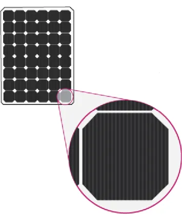
(17) Thèse de Cristian Miron, Université de Lille, 2018. 2. CONSTRUCTION OF THE MATHEMATICAL MODELS 2.1.. Photovoltaic panels. Whenever a model is used in a control loop or a supervisory system, its accuracy plays a crucial role. In this chapter we shall present different typologies of photovoltaic cell models. Before proceeding, a brief reminder of what a solar panel is made of, and how it is functioning will be made. A photovoltaic panel is composed of several photovoltaic cells (Figure 2-1, Figure 2-2 and Figure 2-3). A PV cell captures the energy provided by the sun and transforms into variable DC current. On the present market, we can distinguish three types of technologies that are used for manufacturing them.. Figure 2-1 Monocrystalline solar cells. Monocrystalline solar cells (Figure 2-1) are created from a single continuous crystal structure. The silicon crystal is formed into bars and cut into wafers. Using only one type of crystal offers a higher conductivity to electrons which generate an electric flow, which leads to a lower temperature coefficient. Therefore, it has an increased efficiency of 10÷23% and a better tolerance to higher operating temperatures, with respect to the other technologies presented below. It also requires less space than its homologues.. 16. © 2018 Tous droits réservés.. lilliad.univ-lille.fr.

(18) Thèse de Cristian Miron, Université de Lille, 2018. However, since the fabrication process is more expensive, its final price might represent a drawback for the buyer. They are particularly sensible to shadowing effects if they do not benefit of the bypass diodes devices.. Figure 2-2 Polycristalline solar cells. Polycristalline solar cells (Figure 2-2) are created from fragments of silicon that are melted together to form wafers. Along with the lower purity, the freedom of the electrons to move is diminished as well. This will conduct to a lower efficiency and a higher operating temperature. They have a lower fabrication cost, due to the simplified technology, which makes them more attractive.. Figure 2-3 Thin film amorphous panels. Thin film amorphous panels (Figure 2-3) are created by depositing substances, such as amorphous silicon, cadmium telluride, copper indium gallium selenide or others, on a solid 17. © 2018 Tous droits réservés.. lilliad.univ-lille.fr.

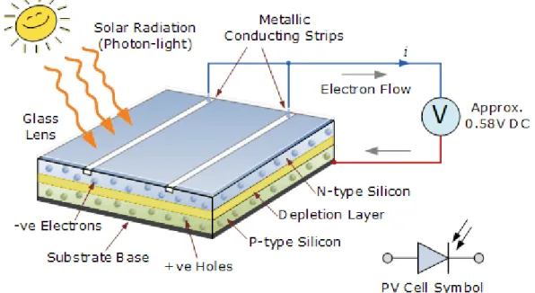
(19) Thèse de Cristian Miron, Université de Lille, 2018. surface. They have an efficiency around 7÷13% and the lowest production cost among the three mentioned technologies. Shadowing effects have a smaller impact over this type of panel, in comparison with the previous two others.. We may associate a PV cell with a PN junction diode, since it is a semiconductor with a positive P type layer and a negative N type later, as presented in Figure 2-4 connected in a series / parallel architecture. When the solar radiation hits the surface of the semiconductor, it sets free electrons that will flow and be collected by the metallic strips. This will represent the positive junction of the PV cell. On the other side, the P-type material, represents the negative junction.. Figure 2-4 PN layer. In order to increase the output voltage of a PV panel, the PV cells are connected in series. To increase the output current, we can either connect the PV cells in parallel, either replace them with others that have a bigger surface area. Photovoltaic arrays, which are obtained by interconnecting multiple PV panels in a series / parallel configuration, can be used to achieve certain power performances. For the next part, the following conventions will be made: is the output current of the PV cell; is the photogenerated current by the incidence of light; is the output voltage of the PV cell; is the diffusion diode current (obtained with the Shockley diode equation); is the recombination diode current; 18. © 2018 Tous droits réservés.. lilliad.univ-lille.fr.

(20) Thèse de Cristian Miron, Université de Lille, 2018. and. are the reverse saturation currents or leakage currents of the diode. and. ;. are the thermal voltages of the two diodes; , where. (. ⁄ ),. is the Boltzmann constant ( ) and. and. ,respectively. is the electron charge. is the temperature of the p-n junction (in Kelvin);. are the ideality factors of the two diodes;. is a series resistance; is a shunt resistance; is the light generated current measured in standard test conditions (STC); is the short circuit current coefficient (measured in. ⁄ );. is the open circuit current coefficient (measured in. );. is the open circuit voltage at STC; is the short circuit current at STC; (temperature measured in Kelvin); is the insolation or irradiance, while. is the irradiance measured in STC.. The performances of a PV panel are measured under standard test conditions (STC): . the photovoltaic cell’s. . the. . air mass of 1.5 spectrum.. ; ⁄. ;. 2.1.1. One diode photovoltaic panel model. Different models of photovoltaic (PV) cells are presented in several paperwork [4,5,8]. The complexity of the chosen model might have a great impact upon the accuracy of the simulation. Thus, the nonlinear I-V and P-V characteristic curves are affected. The simplest (ideal) PV cell model, consisting of a current source ( ) connected in parallel to a diode ( ), offers an output current ( ) directly proportional to the radiation level.. Figure 2-5 Ideal PV cell model. 19. © 2018 Tous droits réservés.. lilliad.univ-lille.fr.

(21) Thèse de Cristian Miron, Université de Lille, 2018. The light generated current can be expressed as: (. (1). ). It can be observed that this term is dependent on both irradiance and temperature. We shall consider, for all further calculus, a constant AM=1.5 atmosphere thickness, which corresponds to a solar zenith angle of 48.2°. We can compute the value of the output current of the photovoltaic cell, by applying Kirchhoff’s current law: (2). where the current of the diode is calculated using the Shockley diode equation: [. (3). ]. The reverse saturation current of the diode can be expressed as following: (. [. *. .. (4). /]. where is the band gap energy of the semiconductor (usually ), while is reverse saturation current at STC.. for polycrystalline. at. Most PV panels datasheets do not offer enough information regarding some of the above mentioned parameters, thus an improved equation which takes into account temperature variation replaces the previous one: (. (5). ) ) (. [(. )]. Replacing the light generated current and the current of the diode from eq.(2) with the values from eq.(1), (3) and (5), we obtain the output current of the ideal photovoltaic cell: (. (. ). ( *. ) ) (. ). (6). [. ]. +. This model has the advantage of having a reduced number of parameters, necessary for computing the I-V characteristic curve. However it presents a big drawback when exposed to environmental variation, fact which makes it unsuitable for real world functioning. An improved model is obtained by adding a series resistance ( ), which takes into account the voltage drops and the internal losses. It is one of the most frequently used models in paperwork and PV cell simulations. 20. © 2018 Tous droits réservés.. lilliad.univ-lille.fr.

(22) Thèse de Cristian Miron, Université de Lille, 2018. Figure 2-6 Rs PV cell model. The output current of the photovoltaic cell is: (7). where the current of the diode becomes:. *. (8). +. When the device operates in the current source region, this model lacks precision. Another model is obtained by adding a parallel resistance ( ) to the previous structure. The I-V characteristic curve of this model is closer to that of the PV cell than in the other cases, by taking into account the leakage current to the ground when the diode is in reverse bias.. Figure 2-7 Rs-Rp PV cell model. The output current of the photovoltaic cell changes to: (. ). (9). It is shown [4] that the one diode PV cell model seems to lack precision when subjected to low voltages, by neglecting the recombination loss in the depletion region of the diode. 2.1.2. Double diode photovoltaic model. Another model is obtained by adding a parallel resistance ( ) to the previous structure. The I-V characteristic curve of this model is closer to that of the PV cell than in the other cases. It is shown [4] that the one diode PV cell model seems to lack precision when subjected to low voltages, by neglecting the recombination loss in the depletion region of the diode. 21. © 2018 Tous droits réservés.. lilliad.univ-lille.fr.

(23) Thèse de Cristian Miron, Université de Lille, 2018. In order to solve this problem a trade-off between the accuracy and the complexity of the model is made. Another diode ( ) is thus added. The two diode PV cell model is presented in Figure 2-8.. Figure 2-8 Double diode PV cell model. The output current (. ) equation of the PV module is:. (. ) (10). *. +. *. +. (. ). It can be observed the number of parameters of this model increased to seven: , , , , , and . In order to reduce the time computation the following simplification is made: ( ) *,(. [(. where. (. ). The values of the 2.1.3.. ,. and and. (11). ) ). -. +]. .. resistances are computed using the algorithm presented in chapter. The reverse saturation current of the two diodes becomes: (. ). [(. ). (12). ]. Typical PV power generation systems are configured in series parallel structures in order to achieve certain power demands. The next equation describes output current of such a x size PV module:. 22. © 2018 Tous droits réservés.. lilliad.univ-lille.fr.

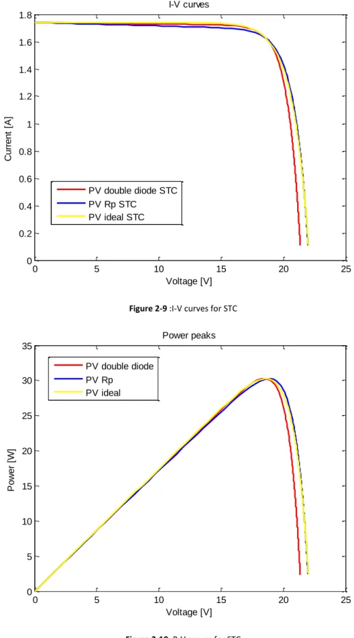
(24) Thèse de Cristian Miron, Université de Lille, 2018. (. *. [. ] ( (. [. *. ] (13). * ,. (. The power of a PV array, the connected load.. (. *. , is dependent on the insolation, the cell temperature and. Different maximum power point tracking (MPPT) algorithms can be found in literature. Their goal is to optimize the efficiency of the PV array by delivering a maximum power that the PV can achieve with respect to the environmental conditions and load. The maximum power point should satisfy the following condition: (14). (. ) (15). [. (. *. (. * (. ] *. A sequence of plots will show the differences between the three types of PV models mentioned earlier for different functioning conditions. The PV panel that is simulated has the characteristics taken from the datasheet of a 30W PV, Ameresco Solar 30J. The I-V curve and P-V curve for STC are presented in Figure 2-9 and Figure 2-10. The same curves are plotted for different values of the irradiation and temperature in Figure 2-11and Figure 2-12.. 23. © 2018 Tous droits réservés.. lilliad.univ-lille.fr.

(25) Thèse de Cristian Miron, Université de Lille, 2018. I-V curves 1.8 1.6 1.4. Current [A]. 1.2 1 0.8 0.6 PV double diode STC PV Rp STC PV ideal STC. 0.4 0.2 0. 0. 5. 10. 15. 20. 25. 20. 25. Voltage [V] Figure 2-9 :I-V curves for STC. Power peaks 35 PV double diode PV Rp PV ideal. 30. Power [W]. 25. 20. 15. 10. 5. 0. 0. 5. 10. 15 Voltage [V]. Figure 2-10: P-V curves for STC. 24. © 2018 Tous droits réservés.. lilliad.univ-lille.fr.

(26) Thèse de Cristian Miron, Université de Lille, 2018. I-V curves 2 75°C,1000W/m² 1.8 STC 1.6. Current [A]. 1.4 1.2. 25°C,600W/m² -15°C, 1000W/m². 1 0.8 0.6 PV double diode PV Rp PV ideal. 0.4 0.2 0. 0. 5. 10. 15 Voltage [V]. 20. 25. 30. Figure 2-11: I-V curves. Power peaks 35 PV double diode PV Rp PV ideal. 30. STC -15°C, 1000W/m². Power [W]. 25 20 75°C,1000W/m² 15 10 25°C,600W/m² 5 0. 0. 5. 10. 15. 20. 25. Voltage [V] Figure 2-12: P-V curves. 25. © 2018 Tous droits réservés.. lilliad.univ-lille.fr.

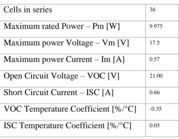
(27) Thèse de Cristian Miron, Université de Lille, 2018. 2.1.3. Graphic user interface A solar panel such as FVG100P can be used for many low budget applications. Having a quick look over the data (Table 2-1) that is provided by the manufacturer one can observe that the values of resistances and are not available. Table 2-1 FVG100P PV datasheet @STC. Cells in series. 36. Maximum rated Power – Pm [W]. 9.975. Maximum power Voltage – Vm [V]. 17.5. Maximum power Current – Im [A]. 0.57. Open Circuit Voltage – VOC [V]. 21.00. Short Circuit Current – ISC [A]. 0.66. VOC Temperature Coefficient [%/°C]. -0.35. ISC Temperature Coefficient [%/°C]. 0.05. A solution for this scenarios is obtained by applying the Newton-Raphson algorithm for finding the values of and described in [1, 2, 8], adapted for the two diode PV cell model. The following graphic user interface (GUI) was developed to facilitate the computation of the two values (Figure 2-13). After filling in the gaps with the data provided in the datasheet of the PV panel and choosing a suitable value for α2 (α1=1, by default) the button that enables the search algorithm can be pressed. The results will be shown among with the I-V and P-V characteristic curves. The simulation is made for a 1500 watts PV array, as in Figure 2-13., while the characteristic curves can be observed in Figure 2-15.. 26. © 2018 Tous droits réservés.. lilliad.univ-lille.fr.

(28) Thèse de Cristian Miron, Université de Lille, 2018. 1 2 4. 3 6. 5. 7 8. 8. Figure 2-13: Graphic User Interface. For configuring the values of irradiance and temperature, we can either use the STC values by checking the radiobutton (4), either we can set them by clicking the “Setup STC/Simulation parameters” button (3). As presented in Figure 2-14, the two parameters can be manually set.. Figure 2-14 Secondary GUI window. Furthermore we can set up the values of the Voc, Vmp and Kv, by filling in the three input boxes from panel (5). We can proceed similarly for setting up the values of Isc, Imp and Ki, from the 27. © 2018 Tous droits réservés.. lilliad.univ-lille.fr.

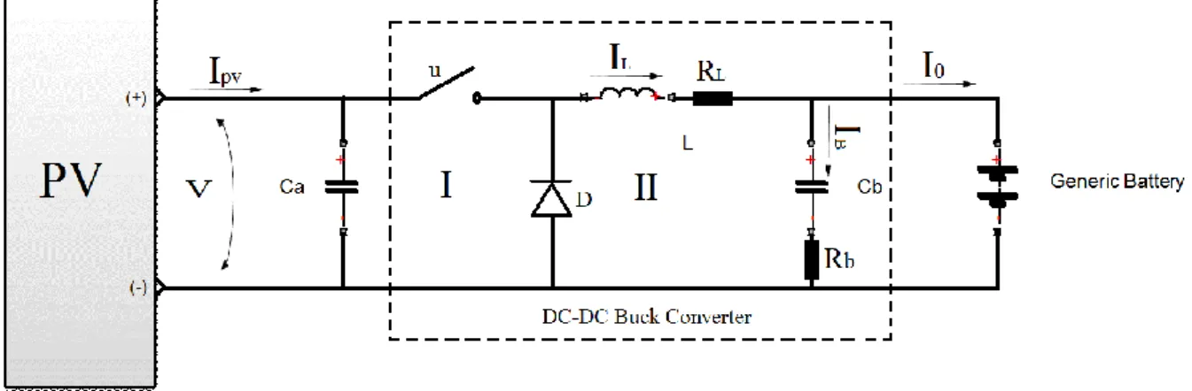
(29) Thèse de Cristian Miron, Université de Lille, 2018. other three input boxes present in panel (6). The input box (7) is used for setting the ideality factor of the second diode. In panel (8) we can decide upon the value of Ns, Np and P, which represents the maximum rated power at STC, for Ns connected PV cells. In order to compute the values of Rs and Rp, using the Newton-Rhapson algorithm, for a model that is using a single/double diode, we have to push the “Compute Rs,Rp” button (8).. The computed values, after applying all the above mentioned steps, are 3.061Ω.. and. Figure 2-15:I-V and P-V characteristic curves. Moreover, we can save the results by pushing the save button (2), and eventually load them later on, by pushing the open button (1).. 2.2 DC/DC converter model 2.2.1 Statespace model. Figure 2-16: DC/DC Buck Converter I. 28. © 2018 Tous droits réservés.. lilliad.univ-lille.fr.

(30) Thèse de Cristian Miron, Université de Lille, 2018. Figure 2-17 DC/DC Buck Converter II. We presume that the PV array is connected to a variable load, a battery in this case. In order to optimize the efficiency of the PV array and to align its voltage to that of the load, a step down converter (DC-DC buck converter) is added, as presented in Figure 2-17. A synchronous buck converter topology is generally preferred, due to a significant reduction of losses. The buck converter is composed of an inductor ( ), a capacitor ( ), a high-side mosfet that is controlled using a pulse-width modulation (PWM) signal – the duty ratio , and a lowside mosfet that is controlled via PWM signal –the duty ratio . The latter component replaces the diode from an asynchronous buck converter topology (Figure 2-16) and offers the advantage of a lower resistance from drain to source which contributes to a higher conversion efficiency. The purpose of this scheme is that the power of the PV array is conserved: . The power losses in a buck converter are caused by the power dissipation in the conduction of the inductor, of the transistors and on the switching losses of the transistors. The voltage drop on the diode is considered, whenever the asynchronous topology is preferred. Furthermore is presented the dynamic model of the buck converter, using state equations. The model will be calculated for the converter presented in Figure 2-16, and finally generalized for both topologies. We shall use the next differential equations of the inductor (eq. 16) and of the capacitor (eq. 17): ( ). ( ). where is the induced voltage on the inductor, current across the inductor.. (16). is inductance, ̇ is the rate of change of the ( ). ( ). (17). where is the current that passes through the capacitor, is the capacitance, ̇ the rate of change of voltage across the capacitor. If we apply them to the inductor and the two capacitors present in Figure 2-18, we shall obtain:. 29. © 2018 Tous droits réservés.. lilliad.univ-lille.fr.

(31) Thèse de Cristian Miron, Université de Lille, 2018. {. (. ). (. ). (18). In order to obtain the value of the inductor’s voltage, , the second law of Kirchhoff is applied between meshes 1 and 2. We shall also consider the internal resistance of the inductor and of the capacitor, as presented in Fig. 2-18.. nd. Figure 2-18 The 2 law of Kirchhoff applied on a DC\DC buck converter. The on state and the off state of the buck converter, when the command u applied on the transistor closes or opens the circuit, are taken into account. (. ) (. (19). ). (20). We shall use the first law of Kirchhoff for calculating the current Ib: (21) (22). If we reintroduce eq. 21 in eq. 20, we obtain: ( (. ). (. ). (23). ). (. ). (24). Eq. 18 can be rewritten as:. 30. © 2018 Tous droits réservés.. lilliad.univ-lille.fr.

(32) Thèse de Cristian Miron, Université de Lille, 2018. (. (. ( {. ). (. )) (25). ). (. ). where : is the output current of the PV array; is the output current of the buck converter; is the current on the inductor ; is the voltage of the PV array on the capacitor is the voltage on the capacitor. ;. ;. is the internal resistance of the inductor ; is the internal resistance of the capacitor. ;. is the PWM signal that controls the transistor(s), that is associated to a given duty cycle; =1-u. The efficiency of the PV array is also affected by the internal resistances is not usually taken into consideration in MPPT paperwork.. and. . This aspect. 2.2.2. Transfer function model. We shall use a simplified version of eq. 25, in order to compute the transfer function of an asynchronous buck converter topology, in continuous mode. The internal resistances of the inductance and of the capacitor, as well as the voltage drop of the diode, are not taken into account. Furthermore, we shall consider for the moment, the variable V as being constant.. Figure 2-19 Simplified DC\DC buck converter. 31. © 2018 Tous droits réservés.. lilliad.univ-lille.fr.

(33) Thèse de Cristian Miron, Université de Lille, 2018. ( ). ( ). ( ). ( ). ( ). (26). ( ). { We shall note the resistance of the generic load with R. ( ). ( ). ( ). ( ). ( ). (27). ( ). { To convert the differential equations in time t into algebraic equations in complex domain s, we will apply the Laplace transform. ( ). ( ) (. ( ). ( ). {. ( ). (. ( ). ( ). ( ) ). ( ). ( ) ). ( )(. (28). ( ). ( ). ( ) *. (29). ( ). (30). (31). Represented in transfer function form, one gets: ( ) ( ). (32). The V variable is not constant so a procedure needs to be implemented in order to solve this. Considering a slower dynamic in the MPPT block, the Vin can be considered to vary slower than the buck converter’s dynamics. As such, we can simply measure its value and divide the obtained command by this measured value.. 32. © 2018 Tous droits réservés.. lilliad.univ-lille.fr.


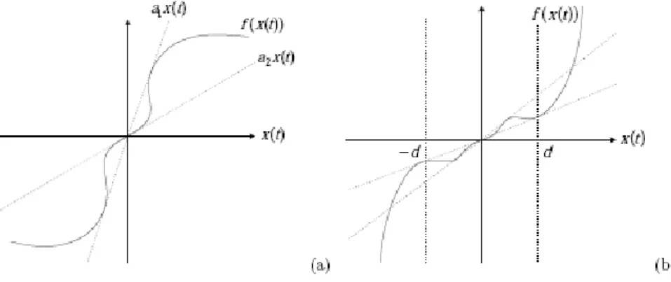
(35) Thèse de Cristian Miron, Université de Lille, 2018. 3. TAKAGI-SUGENO OBSERVER 3.1 TS fuzzy model Most of the physical dynamical systems, which can be represented with differential equations are nonlinear. When the linearization of a system is not representative, this may lead to its instability in a control loop which is not robust enough to compensate all the modelling uncertainties and/or disturbances. A multi-model approach [2] may present a better accuracy of the whole system, especially when the latter is exposed to parameter variations or structural changes for different functioning points. To design a T-S fuzzy observer or controller (Figure 3.1), we need a T-S fuzzy model for a nonlinear system. Therefore, the construction of a fuzzy model represents an important and basic procedure in this approach. Nonlinear System. Physical model. Identification based on input-output data TS Fuzzy model. TS Fuzzy Observer. TS Fuzzy controller. Figure 3-1 Model based fuzzy observer or/and controller. This chapter focuses on the approach based on the idea of "sector nonlinearity", "local approximation," or a combination of them to construct fuzzy models. The idea of using sector nonlinearity in fuzzy model construction first appeared in [8]. This approach guarantees an exact fuzzy model construction. However, it is sometimes difficult to find global sector for general nonlinear systems then local sector nonlinearity is considered. This is reasonable as variables of physical systems are always bounded.. 34. © 2018 Tous droits réservés.. lilliad.univ-lille.fr.

(36) Thèse de Cristian Miron, Université de Lille, 2018. Consider a simple nonlinear system ̇ ( ) ( ), where ( ) =0. The aim is to find the global ( ), sector such that ̇ ( ) -. Figure 3-2 shows the local sector nonlinearity of a function where two lines become the local sectors under ( ) . The fuzzy model exactly represents the local region, that is, ( ) .. Figure 3-2 Local sector nonlinearity. The plant can be described by TS fuzzy [2, 6] plant model without uncertainties and disturbance and can be written in the following form: ̇( ). ∑. ( ( )){. ( ). } (33). ( ). ∑. ( ( )). ( ). ( ) where ( ) is the state vector, is the input vector, ( ) is the output vector, , , are known matrices with appropriate dimensions and r is the number of rules or sub-models. The functions ( ( )) are the weighting functions depending on the state variables ( ) which can be measurable or not measurable variables. These functions verify the so-called convex properties. (34). ∑. ( ( )). ( ( )). *. +. The output equation is chosen to be linear with respect to the state, which is frequently the case in practice. The normalized. functions are given by: ( ( )). The weighting. ∑. ( ( )) ( ( )). (35). functions have the following structure 35. © 2018 Tous droits réservés.. lilliad.univ-lille.fr.

(37) Thèse de Cristian Miron, Université de Lille, 2018. (36). ( ( )). ∏. ( ( )). The membership functions are represented by: ( ) (37). 3.2 TS fuzzy observer A model-based fuzzy observer design utilizing the concept of the Parallel Distributed Compensation (PDC) is used. The concept of PDC technique in [] is utilized to design fuzzy controllers or fuzzy observers to stabilize fuzzy system. The idea of PDC is to associate a compensator for each rule of the fuzzy model. The resulting overall fuzzy observer in our case is a fuzzy blending of each individual linear observer. The fuzzy observer shares the same fuzzy sets with the fuzzy system. It is assumed that the fuzzy system model is locally observable. The PDC is also employed to design the following observer structures. The T-S observer has the following form:. {. ̂̇ ( ) ̂( ). ∑. ( ̂ ( )){. ̂( ). ( ). (. )} (38). ̂( ). where ̂̇ ( ) is the estimated state vector, is the error between the measured signal and the estimated signal, while are the fuzzy observer gains.. 3.3 State space model of PV plant First, a nonlinear PV plant with a Takagi-Sugeno (TS) fuzzy model is presented. Then a modelbased fuzzy observer design utilizing the concept of the Parallel Distributed Compensation (PDC) is used, in which observer gains are obtained by solving Linear Matrix Inequalities (LMIs). The control block based on MPPT algorithm will use in real-time the result provided by the nonlinear observer. Choosing which model or group of models gives the best approximation of the system, with respect to a certain performance criteria, is important. T-S fuzzy model of PV plant The system described in eq. 25 is a non-linear system. A synchronous topology of the buck converter will be preferred, therefore the diode will be replaced with a low side mosfet, as presented in Figure 2-17. The approach that is used in this paper takes into account the number 36. © 2018 Tous droits réservés.. lilliad.univ-lille.fr.

(38) Thèse de Cristian Miron, Université de Lille, 2018. of nonlinearities of the system ( ) and builds a set of linear subsystems ( ) that approximate the initial system. Each linear subsystem will approximate the non-linear system with a certain weight. The state space model is rewritten as below:. (. ). [ ]. [ ] [ ] This can be formalized as the following system: ( ) ̇. where. (. [ ],. [ [. (39). ]. ( ). ). (40). ,. [. ]. [. and. ]. [. ].. ] (41). [ ] where. 0. 1 is chosen with respect to the parameter that will be estimated.. A Takagi-Sugeno (T-S) fuzzy modelling technique [2,6] is used:. {. ̇( ). ∑. ( ). ( ( )){. ( ). ( )}. (42). ( ). where ( ) , ( ) ( ) ( )- contains the nonlinearities of the system, also known as fuzzy variables, and represents the normalized weighting functions. We choose. ,. and. , obtaining a number of r=8 fuzzy rules.. Taking into account these notations the matrixes. (. and. ). from eq. 34 become:. (43). ,. [. ]. [. ]. In the next table are presented the fuzzy rules which help us define the system described in (36). 37. © 2018 Tous droits réservés.. lilliad.univ-lille.fr.

(39) Thèse de Cristian Miron, Université de Lille, 2018. Table 3-1 Fuzzy rules. i. Fuzzy sets. Parameters of then-part. 1 2 3 4 5 6 7 8. zM1 zM1 zm1 zm1 zM1 zM1 zm1 zm1. zM2 zM2 zM2 zM2 zm2 zm2 zm2 zm2. zM3 zm3 zM3 zm3 zM3 zm3 zM3 zm3. 3.4 Lyapunov stability The T-S observer given by (35) is ̂̇ ( ). {. ̂( ). ∑. ( ̂ ( )){. ̂( ). ( ). (. )} (44). ̂( ). ̂ [ ̂ ] [ ], with , measured and ̂ the measured signal and estimated signal. where ̂. estimated ,while. is the error between. The stability of the observer is assured using a Lyapunov stability method [2,6]. This implies the use of a Lyapunov function such as: {. ̂. (45). In order to obtain a bounded error that converges towards zero, the derivative of the function must be negative. ̇ ̇. (46). ̇. The derivative of the error must be computed, using eq. 39 and eq. 42: ̇. ̇. ̂̇. ∑, ( ). ( ̂ )-{. } (47). ∑. ( ̂ )*. (. ̂. ̂)+. 38. © 2018 Tous droits réservés.. lilliad.univ-lille.fr.

(40) Thèse de Cristian Miron, Université de Lille, 2018. ( ̂ )*. ∑ ∑. We consider when ̂ .. +. , ( ). ( ̂ )-{. } as a virtual perturbation that is rejected. The following quadratic stability condition [3] is used: ̇ with. ,. ,. We reintroduce. (48). , and the decay rate. .. 44 in eq. 46 : ̇. (49). ̇. And then we replace the value of ̇ from eq. 45 in eq. 47 and we obtain: (∑. ∑. ( ̂ )*. +. +. ( ̂ ){(. ( ̂ )*. (∑. (. ). +. ). +. }. (50). (51). The next inequality is used: (52). If we consider. ,. and. , eq. 50 becomes: (. ) (. (53). ). The left term of the inequality will be replaced by the right term in eq. 49: ( ̂ ){(. ∑. (. ). ). }. (54). It can be noticed that the term containing the virtual perturbation is reduced. ∑. ( ̂ ){(. (. ). ). }. (55). If we apply the Schur complement lemma we obtain: *. (. ). (. ). +. (56). For obtaining the gains of the observer this linear matrix inequality (LMI) must be solved. This can be easily done solving the LMI with the help of the open source Yalmip toolbox. 39. © 2018 Tous droits réservés.. lilliad.univ-lille.fr.

(41) Thèse de Cristian Miron, Université de Lille, 2018. After computing the gains and , we implement in a simulation environment, such as Matlab/Simulink, the scheme from Figure 2-19 along with the T-S observer. All the presented results are obtained using a variable sampling step. The estimated voltage output of the PV panel approximates well the measured parameter in a short time (Figure 3-). The estimation error converges towards a bounded interval (Figure 3-4) and offers an accuracy superior to 97%.. Figure 3-3 Estimating the output voltage of the PV. 40. © 2018 Tous droits réservés.. lilliad.univ-lille.fr.

(42) Thèse de Cristian Miron, Université de Lille, 2018. Figure 3-4 The estimation error. 3.5. Computing the maximum power point tracking In order to benefit of the maximum power of the PV panel a MPPT control algorithm will be used. Perturb and observe (P&O) algorithm is a popular one and can be found on many controllers used in actual industry. It is easy to implement and has a very simple concept that is described in Figure 4-1. Details about implementation and how the algorithm works can be found the chapter 4. Considering that the dynamic of the observer is faster than that of the control, we can use the estimated voltage computed in real-time with the T-S observer for the MPPT control block. In this way we replace the voltage sensor [7] with a software solution or even integrate a fault detection of that sensor. Using this algorithm the maximum power of the PV panel is achieved under variable irradiance and temperature conditions as it is presented in Figure 3-3.. 41. © 2018 Tous droits réservés.. lilliad.univ-lille.fr.

(43) Thèse de Cristian Miron, Université de Lille, 2018. Power [W]. Power peaks using P&O algorithm 30 20. Temperature [°C]. Irradiance [W/m 2]. 10. 0. 0.005. 0.01. 0.015 0.02 0.025 Simulation time [s]. 0.03. 0.035. 0.04. 0. 0.005. 0.01. 0.015 0.02 0.025 Simulation time [s]. 0.03. 0.035. 0.04. 0. 0.005. 0.01. 0.015 0.02 0.025 Simulation time [s]. 0.03. 0.035. 0.04. 1000 900 800. 20.5 20 19.5. Figure 3-3 Power peaks using P&O algorithm. 42. © 2018 Tous droits réservés.. lilliad.univ-lille.fr.


(45) Thèse de Cristian Miron, Université de Lille, 2018. 4. (MPPT) CONTROL ALGORITHMS 4.1.. Classic control algorithms. As presented in chapter 2, the performances of a PV panel are affected by meteorological conditions, such as irradiance, temperature, air mass spectrum and shadowing. Furthermore, a step down converter architecture is used in order to maximize the quantity of produced energy of the solar panel. In order to achieve this latter objective, several maximum power point tracking (MPPT) control algorithms are proposed. Some of the most popular are the hill climbing based techniques. As the name suggests, these algorithms are using the power-voltage characteristic curve. Among them, we shall remind “Perturb and Observe” (P&O), “Incremental conductance” (IC). The P&O algorithm and different adaptions are widely implemented, due to its simplicity. The system is disturbed at each sampling time and its performances are evaluated. The duty ratio that is used to control the high mosfet of the buck converter is increased or decreased, and then the voltage and the power of the PV panel are measured. Comparing the obtained values with the previous ones we can establish if the power of the PV panel is increasing or decreasing, and how the duty ratio must be adjusted with respect to our goal. By modifying we also modify the value of the output voltage . One of the disadvantages of this technique is that once it finds the maximum power point, it will oscillate around it with an amplitude given by the value of the step size. If this step is fixed, then a pre-calibration under different testing conditions is required. It is also sensible to shadowing effect and variable load changes. In order to construct de MPPT algorithm, a P&O method was implemented based on the logic:. 44. © 2018 Tous droits réservés.. lilliad.univ-lille.fr.

(46) Thèse de Cristian Miron, Université de Lille, 2018. Figure 4-1 The P&O algorithm. The P&O algorithm described in [4,5,6,7] has the advantage of simplicity with satisfying results in tracking. The IC algorithm is another popular algorithm. It computes the control law with respect to eq.14. If , the duty ratio increases, else if , the duty ratio decreases, otherwise the duty maintains its previous value, as presented in Figure 4-2. It has the advantage of eliminating the oscillations around the maximum power point. One of its drawbacks is that is requires more computing resources.. 45. © 2018 Tous droits réservés.. lilliad.univ-lille.fr.

(47) Thèse de Cristian Miron, Université de Lille, 2018. Figure 4-2 The IC algorithm. The next configuration is proposed for the DC-DC converter: the PWM signal will be sent at a frequency of 100kHz, while its inductance , H], the internal resistance of the inductor , -, the capacitance , -, and the internal resistance of the capacitor , -.. yes. A slight advantage can be already noticed. The amplitude of the oscillation when maximum power area is reached is smaller when IC algorithm is used. The difference increases if the step n towards the MPPT. In Figure 4-3 are compared size is chosen for a rather faster conversion rate o the two algorithms, P&O and IC, with two fixed steps: step1=0.5e-5 and step2=1e-6.. 46. © 2018 Tous droits réservés.. lilliad.univ-lille.fr.

(48) Thèse de Cristian Miron, Université de Lille, 2018. P&O vs. IC with constant step size 10 P&O step1 P&O step2 IC step1 IC step2. Power [W]. 9.5 9 8.5 8 7.5 7. 0. 0.005. 0.01. 0.015. 0.02 0.025 Simulation time [s]. 0.03. 0.035. 0.04. Control law 1 P&O step1 P&O step2 IC step1 IC step2. Duty ratio [%]. 0.8 0.6 0.4 0.2 0. 0. 0.005. 0.01. 0.015. 0.02 0.025 Simulation time [s]. 0.03. 0.035. 0.04. Figure 4-3 Comparing P&O with IC algorithm. The duty ratio is similar for the scenario which uses step1 as step size. In order to decrease the time needed for finding the maximum power point a variable step time can be used. In several paperwork [7] this objective is achieved by multiplying a constant step size with. .. In spite of the faster initial convergence rate (Figure 4-3) the result is similar to one obtained with IC with constant step size. An improved IC algorithm is proposed in the following part. Increasing or decreasing the duty ratio is accomplished by adding or subtracting a certain value, often called step, from the previous duty ratio . As presented earlier, if the step size is fixed, then the standard IC algorithm is used. If the step size is variable, such as , then a IC with variable step size is used. However, an improvement can be added by combining the two methods with respect to the dynamic of the step size. Measuring the last three values of (|. ( ). |. provides information about the search direction: |. (. ). |) (|. If eq. 55 is greater than or equal to zero and | | ( ). (. ). |. |. (. ). |). (57). , then the step size becomes: (. ). (58). 47. © 2018 Tous droits réservés.. lilliad.univ-lille.fr.

(49) Thèse de Cristian Miron, Université de Lille, 2018. where ratio is a finite number and algorithm is increased. If | |. is the domain in which the acceleration of the search. the step size becomes constant (. ).. Otherwise if eq. 55 is smaller than zero the step size becomes constant ( For better performances it is advised that ( ) is smaller than (. ).. ).. In Figure 4-4 are compared the above mentioned cases, with three different step sizes. It can be observed that the improved IC algorithm has a faster conversion rate and oscillations with really small amplitude, aspect that can be confirmed by the control law. IC with constant step size vs. IC with variable step size vs. IC improved 10 IC step1 IC variable step IC improved. Power [W]. 9.5 9 8.5 8 7.5 7. 0. 0.005. 0.01. 0.015. 0.02 0.025 Simulation time [s]. 0.03. 0.035. 0.04. Control law 1 IC step1 IC variable step IC improved. Duty ratio [%]. 0.8 0.6 0.4 0.2 0. 0. 0.005. 0.01. 0.015. 0.02 0.025 Simulation time [s]. 0.03. 0.035. 0.04. Figure 4-4 Comparing improved IC with other IC algorithms. 48. © 2018 Tous droits réservés.. lilliad.univ-lille.fr.


(51) Thèse de Cristian Miron, Université de Lille, 2018. 4.2 Advanced control algorithms (robust polynomial algorithms) 4.2.1 RST regulator for the Buck Converter 4.2.1 RST regulator for the Buck Converter. In Figure 4-5 is presented the general schematic of the architecture. In this simulation, the main load connected to the buck converter is a resistive load (as a heating element or light bulbs). To maintain the continuity of the schematic between the two converters, an auxiliary resistance is added. This can represent a cooling unit or local lighting.. Figure 4-5 The overall system architecture. Considering the transistor in the buck converter, its switching affects the other converter as well, as a continuous variation of the equivalent impedance. As such, the current oscillates, but its mean value remains constant for a constant input voltage. The buck converter works with a 32Khz frequency command. The inductance value is chosen accordingly, with a value of 160 [µH]. The condensers, at the output we have 220 [µF], and at the input 100 [µF] to smoothen the input. The transfer function of the process was presented in eq. 32: (59). ( ) where. ,. -,. ,. - and. , -.. The mathematical model of the discretized process is an auto-regressive model with exogenous input (ARX). After using the “zero order hold” discretization method [55] the following discrete transfer function of the model is obtained for a sampling time of 62.5 : (. ). ( (. ) ). ( (. ). (60). ). 50. © 2018 Tous droits réservés.. lilliad.univ-lille.fr.

(52) Thèse de Cristian Miron, Université de Lille, 2018. The dynamic of the process can be observed in figure presented below.. Figure 4-6 Step response of the plant model. A polynomial R-S-T algorithm ( [53],[55],[56] ) is proposed for controlling the plant model above. The demanded performances are adjusted through some trials simulating the behavior of the global system, including the photovoltaic generator, the converters, variable solar irradiation and temperature.. Figure 4-7 RST feedback diagram. 51. © 2018 Tous droits réservés.. lilliad.univ-lille.fr.

(53) Thèse de Cristian Miron, Université de Lille, 2018. This control structure takes into account the discretized transfer function of the process, the R-ST polynomials used for controlling the plant in closed loop and rejecting the disturbances, and the trajectory generator which imposes a desired trajectory. The general RST command form is the following: ( (. ( ). ) ( ) ). ( (. ) ( ) ). (61). Where the polynomials of the controller are defined as below: ( { ( (. ) ) ). (62). The polynomials of the plant are defined as below: ( (. {. ) ). (63). The coefficients of the plant can be substituted with the values obtained in eq. 58. Further we can compute the transfer function of the closed loop system (. ). (. ) (. ( ). ) (. ) (. ( ) (. ). ) ( ( ). ) (64). where the poles of the closed loop system are characterized by the polynomial: (. (65). ). The polynomial P contains the dominant and auxiliary poles of the closed loop system: (. ). (. ) (. ). (. ) (. ). (. ). (. ). (66). ( ) corresponds to the dominant closed loop poles of the system, and is responsible with for performances of the controller. ( ) stands for the auxiliary poles of the closed loop system, which are used for filtering purposes, for the improving the robustness of the system. As mentioned in [30], the auxiliary poles are faster than the dominant poles, meaning that the a real part of the roots of ( ) is inferior to one of ( ). A second degree transfer function is usually used for imposing the dominant poles, thus the desired behavior of the closed loop system. (67). ( ) where , is the damping factor and. is the natural frequency.. Taking into account the value of the sampling period (62.5 μs), a damping factor natural frequency rad/s are chosen.. and a. After the discretization we obtain: 52. © 2018 Tous droits réservés.. lilliad.univ-lille.fr.