Reliability of a Hydrodynamic Journal Bearing

This is an author-deposited version published in: https://sam.ensam.eu

Handle ID: .http://hdl.handle.net/10985/10285

To cite this version :

Khadim DIOP, Abdérafi CHARKI, Stéphane CHAMPMARTIN, Abdelhak AMBARI - Reliability of a Hydrodynamic Journal Bearing - In: International Conference on Fluid Dynamics (ICFD 2015), Etats-Unis, 2015-04 - International Conference on Fluid Dynamics - 2015

Any correspondence concerning this service should be sent to the repository Administrator : archiveouverte@ensam.eu

Reliability of a Hydrodynamic Journal Bearing

Khadim DIOP

, Abdérafi CHARKI

,Stéphane CHAMPMARTIN,

and Abdelhak AMBARI

1

62 Avenue Notre Dame du Lac, 49000 Angers, France 2

62 Avenue Notre Dame du Lac, 49000 Angers, France 3

2 Boulevard du Ronceray, 49035 Angers Cedex, France a

khadimdiops@hotmail.com, babderafi.charki@univ-angers.fr, cstephane.champmartin@ensam.eu, d

abdelhak.ambari@ensam.eu

Keywords: Hydrodynamic Journal Bearing, FORM, SORM, Monte Carlo, Function of performance,

Probability of Failure, Reliability.

Abstract. Journal fluid bearings are widely used in industry due to their static and dynamic behavior and their very low coefficient of friction. The technical requirements to improve the new technologies design are increasingly focused on the indicators of dependability of systems and machines. Then, it is necessary to develop a methodology to study the reliability of bearings in order to improve and to evaluate their design quality. Few works are referenced in literature concerning the estimation of the reliability of fluid journal bearings. This paper deals with a methodology to study the failure probability of a hydrodynamic journal bearing. An analytical approach is proposed to calculate static characteristics in using the Reynolds equation. The commonly methods used in structural reliability such as FORM (First Order Reliability Method), SORM (Second Order Reliability Method) and Monte Carlo are developed to estimate the failure probability. The function of performance bounding two domains (domain of safety and domain of failure) is estimated for several geometrical configurations of a hydrodynamic journal bearing (long journal bearings with the hypotheses of Sommerfeld, Gümbel and Reynolds, and a short journal bearing with the hypothesis of Gümbel). Introduction

Fluid bearings are sensitive components for machines and systems. The design of a fluid bearing is usually based on deterministic static characteristics. However, it is subjected to load and pressure fluctuations or to fluid film gap perturbations induced for instance by defects of the slide ways surfaces geometry [1, 2, 3]. The prediction of the reliability of a fluid bearing under operating conditions is then necessary for applications requiring high accuracy movements or positioning [1]. Charki and al. [1, 2,4] developed a methodology to estimate the failure probability of a thrust fluid bearing and a hemispherical fluid bearing.

The literature is sparse regarding research that investigates the reliability estimation of such mechanical component. Charki and al. [1, 2,4] published the first works in this field concerning especially a thrust air bearing [2] and a hemispherical air bearing [4].

Frêne and al. [5] developed an analytical approach with the assumptions of Sommerfeld, Gümbel and Reynolds. Nathi Ram and al. [6] analyzed the behavior of a hybrid journal bearing. An experimental assessment of hydrostatic thrust bearing performance was done by Osman and al. [7].

In reliability analysis, the principle consists in the approximation of a limit-state function bounding two domains (domain of safety and domain of failure). Lemaire and al. [8], detailed the various evaluation methods of the probability of failure. Madsen [9] and Melchers [10] proposed several examples of the estimation of the failure probability. Austin [11] studied the cause of the bearings failures in engines. This paper presents an adapted method to evaluate the failure probability of a journal fluid bearing (see Fig. 1). The methodology is applied to various geometrical configurations of a hydrodynamic journal bearing.

All rights reserved. No part of contents of this paper may be reproduced or transmitted in any form or by any means without the written permission of Trans Tech Publications, www.ttp.net. (ID: 130.237.29.138, Kungliga Tekniska Hogskolan, Stockholm, Sweden-11/09/15,01:31:55)

Fig.1 Journal bearing Nomenclature

Velocity vector of the fluid (m/s). t Time (s).

ρ Lubricant density (kg.m-3

) .

P Hydrodynamic pressure (Pa).

μ Lubricant viscosity (Pa.s).

u, v, w Components of the lubricant velocity in the x, y, and z directions respectively (m/s). x, y, zCoordinates.

u v w Components of the lubricant velocity on the bearing. u v w Components of the lubricant velocity on the shaft.

h Film thickness (m). R Journal radius (m) D Journal diameter (m).

L length of long journal bearing with conditions Sommerfeld, Gümbel and Reynolds (m). Lc Length of short journal bearing (m).

ωAngular velocity of the journal (rad/s).

δAngle between the direction of the coordinate of the component of the following speed x and the direction of the linear speed (°).

R , R Radius respectively of shaft and bearing (m). O , O Center respectively of shaft and the bearing.

e Distance of the centers or eccentricity (m).

C Radial clearance (m).

X Variables of design corresponding to μ, ω, L, L , R, C P Lubricant inlet pressure (Pa).

ε Eccentricity ratio. β Index of reliability. U∗ _{Design point.}

P Pressure of Sommerfeld (Pa). P Pressure of Gϋmbel (Pa). P Pressure of Reynolds (Pa).

θ Angular coordinate at the break of fluid (°).

W ,W , W , W Nominal load capacity (N).

W , W , W , W Critical load capacity respectively of long journal bearing with Sommerfeld, Gümbel, Reynolds conditions, and of Short bearing.

Journal Bearing Modeling

The Reynolds equation [5] is obtained as follows: Equation of conservation of mass:

∇. V = 0 (1) Equation of momentum conservation:

∂V

∂t + V. ∇ . V = −1ρ ∇P +μρ ∇ V (2) Where V the velocity vector of the fluid with componentsu, v, w ; t represents the time; P is the pressure of the fluid. The boundary conditions are [5]:

y = 0 u = u ; v = 0 ; w = w and for y = h u = u ; v = v ; ; w = w The equation of Reynolds is expressed as:

ℎ

+ ℎ

= 6( − ) ℎ+ 6( − ) ℎ+ 6ℎ ( + ) + 6ℎ ( + ) + 12 + 12ℎ ℎ (3)

The hypotheses relative to the stationary equation of Reynolds which allows to write the laminar flow of a fluid between two walls very close and being able to be in movement are given by [5].

Fig. 2 Movement between shaft and bearing By geometrical considerations (see Fig. 2), we have:

u = ωRcosδ (4) v = ωRsinδ (5) For an angle δ very small, the velocity components become:

v = ωR∂h_{∂x (7)} The Reynolds equation becomes:

∂

∂x hμ ∂P∂x +∂z∂ hμ ∂P∂z = 6ωR∂h∂x (8)

Expression of the film thickness

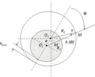
We consider a point M belonging to the surface of the bearing and located by the angle (MO , MO ) with O et O respectively the centers of the pivot shaft and the bearing (see Fig. 3). The point M’ is the orthogonal projection of O on the line ( O M).

Fig. 3 Film thickness between shaft and bearing

Taking into account the relative eccentricity ε = varying from 0 to 1, the expression the film thickness h(θ) becomes then:

h(θ) = C(1 + ε cosθ ) (9) Long bearing with Sommerfeld conditions

The boundary conditions of Sommerfeld [5] are defined as: P ( θ = 0, z ) = P

P (θ = 2π, z ) = P

The Reynolds equation for a long cylindrical bearing with Sommerfeld conditions becomes: ∂

∂x hμ ∂P∂x = 6ωR∂h∂x (10) With x = Rθ, replacing h(θ) = C(1 + ε cosθ ) in the (Eq. 10) and according to an integration of 2π we obtain:

P = 6μω (1 − ε )

R

C ψ − ε sinψ −ψ(2 + ε ) − 4εsinψ + ε sinψcosψ2 + ε + P (11) The load capacity with Sommerfeld conditions is expressed as:

W = 12πμωR Lε

C (2 + ε )(1 − ε ) (12) Long bearing with Gümbel conditions

Boundary conditions of Gümbel [5] are defined as: P (θ = 0, z ) = 0 P (θ = π, z ) = 0 P (θ, z ) = 0 si π < < 2 P = 6μω (1 − ε ) R

C ψ − ε sinψ −ψ(2 + ε ) − 4εsinψ + ε sinψcosψ(1 − ε ) + P (13) The integration of the pressure on the surface of the journal bearing gives the following expression of load capacity with Gümbel conditions:

W = 6μωL R_C ε (4ε + π ( 1 − ε ))_{(2 + ε ) (1 − ε )} (14)

Long bearing with Reynolds conditions

Boundary conditions of Reynolds [5] are defined as: P(θ = 0, z) = P P(θ = 0, z) = 0 ∂P ∂θ ( θ = θ , z) = ∂P∂z ( θ = θ , z) = 0 P (θ, z ) = 0 si θ < < 2 P = 6μω (1 − ε ) R

C ψ − εsinψ −ψ(2 + ε ) − 4εsinψ + ε sinψcosψ2(1 − εcosψ ) (15) The equation of the fluid break is given:

ε(sinψ cosψ − ψ ) + 2(sinψ − ψ cosψ ) = 0 (16) The load capacity with Reynolds conditions is expressed as:

W = 3μωRL (1 − εcosψ )(1 − ε )

R

C ε (1 − cosψ )1 − ε + 4(sinψ − ψ cosψ ) (17) Short journal bearing

The two main hypotheses allowing the justification of a short journal bearing are:

The ratio of the length on the diameter of the bearing is low ≤ . The gradient of pressure at the circumference is negligible compared to the axial pressure [5].

Taking into account these hypotheses, the equation of Reynolds for a short journal bearing becomes: ∂

∂z ρhμ ∂P∂z = 6ωdhdθ (18) P θ, Z = ± L 2 = 0 (19) We obtain finally for short bearing conditions, the expression of the pressure and the load capacity: P(θ, z) = −3μω_C z −L_{4 (1 + εcosθ) (20)}εsinθ W =μRωL_{4C (1 − ε ) (π (1 − ε ) + 16ε ) (21)}ε

Principle of reliability

Causes and failure modes of journal bearings

Failure modes are generally a combination of constraints which act on the bearing until causing a damage or a failure modes are noticed the incapacity of the component bearing to perform a required function. We distinguish essentially failure modes due to corrosion or fatigue, or misalignment of the shaft in the bearing [11].

The evaluation of failure probability bearing [1, 2, 4] can be made by the determination of a limit function separating two zones (domain of safety, domain of failure). In the case of a fluid bearing, the function G is the difference between a nominal load capacity and a critical load capacity.

Limit state function G

The reliability of a journal bearing is defined by the knowledge of a function state limit G(X ), variables of design X chosen as random variables. The considered design variables of design are the viscosity, the angular velocity, the radial clearance, the length and the diameter of bearing. The domains of the performance function [8, 9] are defined as:

G(Xi) > 0 is the domain of safety; G(Xi) < 0 is the domain of failure; G(Xi) = 0 is the limit state;

The function performanceG(L, R, C, ω, μ) depends on 5random variables .It is the difference between the maximal load capacity corresponding a critical eccentricity and the nominal load capacity. Hasofer and Lind [12] show that the index of reliability is the minimum of the distance between the origin and the space of variables normalized with the constraint H(U ) where H the function of performance in the reduced centered standardized space (see Fig. 4).

Fig. 4 Transformation into standard normal space

m and m are respectively the average of variables X and X in the physical space. This is the transformation of the passage of the physical space in the standardized space.

X U =x − m_σ (22) U : Random variable in the gaussian standardized space

σ : Standard deviation of the random variable X . Algorithm of Rackwitz-Fiessler

The algorithm developed by Rackwitz and Fiessler is based on the calculation of the gradients of every variable. Knowing the gradients, we can then estimate linearly the design point, and take the same strategy around this new point P* until convergence by taking place in the point U corresponding to the design point of the iteration k, we can write the development of Taylor around this point of the function H(U) [8]:

H(U) = H U∗ _{+ ∇H(U) ∗ U − U}∗ ₍₂₃₎

By this formula, we can estimate the design of the following iteration:

H U∗ _{= H U}∗ _{+ ∇H(U) ∗ U}∗ _{− U}∗ _{= 0 (24)}

We introduce the vector of the cosine director α:

α =_{‖∇H(U)‖ (25)}∇H(U) The limit state takes the following shape:

∇H(U∗ ₎

‖∇H(U)‖ ∗ + U

∗ _{− U}∗ _{α = 0 (26)}

U∗ _{α = U}∗ _{α −} ∇H U∗

‖∇H(U)‖ ∗ (27)

By introducing the index of reliability into the last equation, it is transformed by: β = U∗ _{α −} ∇H U∗

‖∇H(U)‖ ∗ (28)

We can then estimate the new design point:

U∗ _{= −β α (29)}

The algorithm stops when:

β − β < ε (30) The gradient H(U∗ ) is then given as:

∇H U∗ ₌ H U∗ − H U∗

U∗ _{− U}∗ (31)

FORM

FORM (First Order Reliability Method) approximates the domain of failure by a half-space bounded by a hyper tangent plan on the surface in the design point.

P = φ(−β) (32) φ: standard normal distribution

The design point is the solution of the problem of optimization: β = min U U

H(U) = 0 (33) The result of this problem of minimization under constraint will be solved by the algorithm of Rackwitz-Fiessler and the design point estimated as:

U∗ _{= −α β (34)}

The equation of the tangent hyperplan in the design point U∗ is:

SORM

The SORM (Second Order Reliability Method) consists in approaching the surface of state-limit by a quadratic surface. This method consists in determining an approximation of the function performance H(U), noted Ĥ(U) by a development of Taylor around a given point U .

H(U) = H(U ) + a (U − U ) +1_{2 (U − U ) ℍ(U )(U − U ) + O(‖U − U ‖ ) (36)} The Hessian matrix ℍ owes to be determined then diagonalized so that the main curvatures k can be calculated.

H(U) = U − β −1₂ k U (37) The probability of failure can be estimated by the following relation:

P = φ(−β) (1 + k β) (38)

Monte Carlo method

Methods of simulation allow estimating the probability of failure in the case of complex laws of probability, correlations between variables or function of non linear limit states

P ≈_N1 I G(X ) ≤ 0 (39) Where X is the vector of random variables and I is the indicator function which is equal to 1 if the condition G(X ) ≤ 0 is true and equal to 0 if not.

Applications

Table.1 presents all random variables taken into account for the evaluation of failure probability. For each condition (Sommerfeld, Gümbel, Reynolds, Short Bearing), the failure probability is estimated using the function of performance which is the difference between a critical load capacity and an operating load capacity.

Table 1. Random variables Variables Xi Meanm Standard

deviation σ

Distribution

μ(Pa.s) 12E-4 12E-5 Normal

ω(radian.s-1 ) 157 15.7 Normal L(m) L (m) 0.0125 0.5 1E-5 1E-5 Normal Normal R(m) C(m) 40E-6 5E-2 1E-4 40E-7 Normal Normal

Fig. 5 Failure probability versus relative eccentricity for Sommerfeld conditions

Fig. 6 Failure probability versus relative eccentricity for Gümbel conditions

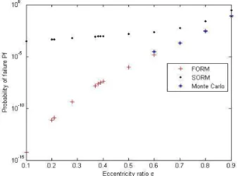
Fig. 7 Failure probability versus relative eccentricity for Reynolds conditions

Fig. 8 Failure probability versus relative eccentricity for short bearing

For the approximation of Sommerfeld, the probability of failure is estimated according to a critical load capacity corresponding to a relative eccentricity ε = 0.95. Figures 5, 6, 7, 8 show the failure probability versus the relative eccentricity. The probability of failure is lower than 10 for lower relative eccentricities than 0.6 according to the results given by FORM and SORM. The results of Monte Carlo for the relative eccentricities higher than 0.6 give values of the probability of failure in agreement with FORM results. The probability of failure increases for a decrease in index of reliability which represents the distance of the origin to the point design.

For the approximation of Gümbel, the probability of failure remains acceptable for values of eccentricities higher than 0.7. The probability of failure decreases exponentially with the increase in the values of the index of reliability in the case of the three methods (FORM, SORM and Monte Carlo). In the case of short journal bearings, the best adapted conditions are the ones of Gümbel according to Dubois and al. [13].

Conclusion

In this paper, we propose a suitable methodology to estimate the reliability of a journal bearing. An analytical approach is developed for the calculation of load capacity of a journal bearing using a combination of the principle of reliability. FORM, SORM and Monte Carlo simulation are used to estimate failure probability of a journal bearing. The methodology can be used for different configurations (different geometry and type of fluid) of fluid bearings in order to improve its design.

References

[1] Charki A., Elsayed E. A., Guerin F., Bigaud D., “Fluid thrust bearing reliability analysis using finite element modeling and response surface method”, International Journal of Quality Engineering and Technology, Vol. 1, pp. 188-205, 2009.

[2] Charki A., Diop K., Champmartin S., Ambari A., “Reliability of a Hydrostatic Bearing”, Journal of Tribology Vol. 136, 2014.

[3] Charki A., Diop K., Champmartin S., Ambari A., “Numerical simulation and experimental study of thrust air bearings with multiple orifices", International Journal of Mechanical Sciences, Vol. 72, pp. 28-38, 2013.

[4] Charki A., Bigaud D., Guérin F., “Behavior analysis of machines and system air hemispherical spindles using finite element modeling, Vol. 65/4, pp. 272-283, 2013.

[5] Frêne F., Nicolas D., Degueurce B., Berthe D., Godet M., “Hydrodynamic Lubrication, bearing and thrust bearings”, Elsevier, Tribology Series, 33, Editor D. Dowson, 1997.

[6] Nathi Ram, Satish C, Sharma. Analysis of orifice compensated non-recessed hole-entry hybrid journal bearing operating with micropolar lubricants. Tribology international 52 (2012) 132-143. [7] Osman T. A., Dorid M., Safar Z. S., Mokhtar M. O., “Experimental assessment of hydrostatic

thrust bearing performance”, Tribology international, Vol. 29/3, pp.233-239, 1996. [8] Lemaire M., Chateauneuf A., Mitteau J-C., Structural Reliability, Wiley on Library, 2010. [9] Madsen H. O., Krenk S., Lind N. C., Methods of Structural Safety, Prentice-Hall, Upper Saddle

River, New Jersey, 1986.

[10] Melchers R. E., Structural reliability: analysis and Prediction, Second Edition, John Wiley and Sons, New York, 1999.

[11] Austin H., Bonnet, U.S Electrical Motors. Cause And Analysis of the Failure of bearings Antifriction In Engines A Induction CA.

[12] Hasofer A. M., Lind N. C., Exact and invariant second-moment code format, Journal of Engineerg in Mechanics, ASCE, Vol. 100/1, pp. 111-121, 1974.

[13] Dubois G. B., Ocvirk F. W., Wehe R. L., Study of Effet of a Non-Newtonian Oil on Friction and Eccentricity Ratio of a Plain Journal Bearing, National Aeronautics and Space Administration, 1960.