BART applied to insurance

Université de Montréal

BART applied to insurance

par

Catherine Paradis-Therrien

Département de mathématiques et de statistique faculté des arts et des sciences

Mémoire présenté à la Faculté des études supérieures en vue de l’obtention du grade de

Maïtre ès sciences (M.Sc.) en Statistique

octobre 200f

L

Université

de Montréal

Dh-ection des bibhothèqiies

AVIS

L’auteur a autorisé l’Université de Montréal à reproduite et diffuser, en totalité ou en partie, par quelque moyen que ce soit et sur quelque support que ce soit, et exclusivement à des fins non lucratives d’enseignement et de recherche, des copies de ce mémoire ou de cette thèse.

L’auteur et les coauteurs le cas échéant conservent la propriété du droit d’auteur et des droits moraux qui protègent ce document. Ni la thèse ou le mémoire, ni des extraits substantiels de ce document, ne doivent être imprimés ou autrement reproduits sans l’autorisation de l’auteur.

Afin de se conformer à la Loi canadienne sur la protection des renseignements personnels, quelques formulaires secondaires, coordonnées ou signatures intégrées au texte ont pu être enlevés de ce document. Bien que cela ait pu affecter la pagination, il n’y a aucun contenu manquant. NOTICE

The author cf this thesis or dissertation has granted a nonexclusive license allowing Université de Montréal to reproduce and publish the document, in part or in whole, and in any format, solely for noncommercia? educational and research purposes.

The author and co-authors if applicable retain copyright ownership and moral rights in this document. Neither the whole thesis or dissertation, nor substantial extracts from it, may be printed or otherwise reproduced without the author’s permission.

In compliance with the Canadian Privacy Act some supporting forms, contact information or signatures may have been removed from the document. While this may affect the document page count, it does flot represent any loss of content from the document.

Université de Montréal

Ce mémoire intitulé

BART applied to insurance

présenté par

Catherine Paradis-Therrien

a été évalué par un jury composé des personnes suivantes charles D ugas (président-rapporteur) Jean-François Angers (directeur de recherche) Yves Lepage (membres du jury) Mémoire accepté le:

111

SOMMAIRE

Ce mémoire porte sur deux méthodes de forage de données (data mining) ap pliquées au domaine de l’assurance. Afin de mieux comprendre les données. deux méthodes «analyse en grappes soient les analyses hiérarchiques et non hiérar

chiques. sont utilisées. Ensilite, des arbres de décision sont développés eu util isant le ratio de vente comme variable dépendante. Le but de ces modèles est de prédire les acheteurs de produits «assurance les plus probables. Pour ce faire. les algorithmes de construct ion selon l’approche classique et 1 ‘approche bayésienne sont confrontés. Ainsi. l’approche classique utilise un algorithme de construc tion qui minimise une fonction d’impureté lors de chaque séparation. L’approche bayésienne quant à elle utilise plusieurs distributions a priori telles que celles des variables et du nombre de noeuds terminaux. L’objectif dans ce cas est de trouver l’arbre ayant la probabilité a posteriori la plus grande possible. Une fois que les arbres ont été construits selon les deux approches, les résultats sont comparés afin de déterminer quelle est celle qui donne les meilleurs arbres.

iv

$UMMARY

ihis Masters thesis presents two data mining techniques applied in the insurance business. First. hierarchical and partitional clustering are used to have a better knowledge of the population under consideration. Then. in order to predict the most potential buyers. we consider the decision tree models with the closing ratio as the target variable. These trees are developed using the classical and tue Ba esian statistical approaches. The classical n;etÏiod algorithu; constructs CART models hy minirnizing an impurity function. On the other hand. the Bavesian approach uses rnany priors as the variable priors or the tree shape prior to construct trees with the n;aximuni posterior probahihty. Once the trees are developed under these two approaches. the resuits are compared to determine which method gives the best trees.

V

CONTENTS

Chapter 1. Insurance and statistical notions 6

1.1. Objectives 6

1.1.1. Direct Market population 6

1.1.2. Model the closing ratio 7

1.2. Definitions 7

1.3. Variables and database 9

1.3.1. Demographic variables 10

1.3.2. Automobile variables 10

1.3.3. Residential variables 12

1.1. Descriptive analvsis 12

1.4.1. Descriptive analysis for Ontario 13

1.4.1.1. Demographic variables 13

1.4.1.2. Automobile variables 13

vi

1.1.2. Average closing ratio. 16

1.5. EM Algorithm for a Mixture Model . 16

Chapter 2. Classical approach 19

2.1. Clustering 19

2.1.1. Description 20

2.1.2. Preparing the data 21

2.1.3. Similarity measure hetween individuals 22 2.1.3.1. Similarity measure for quantitative variables 23 2.1.3.2. Similarity measure for ordinal variables 23 2.1.3.3. Similarity measure for binar variables 24

2.1.4. Distance measure between clusters 2.5

2.1.5. Clustering strategies 26

2.1.5.1. Hierarchical clustering 27

2.1.5.2. Partitional clustering with K-rneans clustering 30

2.1.6. Number of clusters in K-means 32

2.2. Decision trees 35

2.2.1. Description 36

2.2.2. Construction 39

2.2.3. Set of questions 40

2.2.4. Data considerations for the splits 40

2.2.5. Coodness of spiit 41

2.2.5.1. The entropy impurity 43

2.2.5.2. The Gini inipurit.v 43

2.2.5.3. The misclassification irnpuritv 45

2.2.6. Pruning 45

2.2.7. Stopping rules 16

vii

2.2.7.2. IViinirnal change in impurity. 46

2.2.8. Model assessment 48

2.2.9. Advantages and disadvantages (Breiman et aL. 1984) 49

Chapter 3. Bayesian approach 52

3.1. Bayesian theory 53

3.2. BART structure 54

3.3. Distributions of the predictors 58

3.4. Distribution of the variable of interest y 62

3.5. Specification of the tree prior 63

3.5.1. Prior on variables 64

3.5.2. Prior on splitting values 65

3.5.3. Prior for the number of termina.l nodes 66

3.6. Posterior distributions 69

3.6.1. Posterior distribution on tree 69

3.6.2. Posterior distribution for the choice of the spiit variable 69 3.6.3. A posterior density for the choice of the spiit value 70

3.7. Construction of the trees 71

3.7.1. Growillg 72

3.7.2. Pruning 72

3.7.3. Stay 73

3.7.4. Specification of the algorithm 73

3.8. Assigiling classes to terminal nodes 74

3.9. Criteria for tree selection 75

3.9.1. Posterior probability of the tree 75

viii 3.9.3. Misclassification rates. 76 Chapter 4. Resuits 80 4.1. Classical Resuits 81 4.1.1. Clustering 81 4.1.1.1. Description $2 4.1.2. Decision tree $2 4.1.2.1. Impurity 83 4.1.2.2. Stopping rule 83 4.1.2.3. Splitting rule $4

4.1.2.4. Tree from the pure classical approach 85 4.1.2.5. Tree from the combination approach 90 4.1.2.6. Comparison between the two classical techniques 96

4.2. Bayesian Resuits 96

4.3. Comparison between classical and Bayesian approaches 105

4.3.1. Interpretahility 105

4.3.2. Misclassification rates 106

Conclusion 108

ix

LIST 0F FIGURES

1.1 Histogram of the variable “age” 14

1.2 Density of a mixture of two normal variables 17

2.1 Deudrogram produced by hierarchical clustering on Example 2.1.1 28 2.2 Deudrogram produced by hierarchical clusteriug and choice of the

cutting value 29

2.3 Illustration of the K-meaus algorithm 31

2.4 Represeutatiou of the CART model 37

2.5 Tree model 011 Example 2.1.1 38

2.6 Node impurity measures for two-class classification 44

2.7 Example of tree fully growu 47

3.1 BART structure on Example 2.1.1 55

3.2 BART with two levels and 7 terminal uodes 57

3.3 Histogram for a normal deusity with 6 0 and u = 1 59 3.4 Histogram for a gamma deusity with u = 1.5 aud /3 = 2 60 3.5 Histogram for a mixture of two gamma densities with o = 1.5, 3 = 3.

u2=17,82=7andp=0.4 60

3.6 Bar chart of a Poisson deusity with parameter À 1 61 3.7 Example of two trees with the same number of terminal nodes but with

differeut shapes 68

X

1.1 Ontario cluster distribution in 2005 using the K-means algorithm with

the centroid distance 81

4.2 Root node and first level of the CART model using the pure classical

approach 86

4.3 Left suhtree of the pure CART model 87

4.4 Middle subtree of the pure CART model 88

4.5 Complete pure CART model 89

4.6 Root node and first level for the combination approach 90

4.7 Left subtree for the combination approach 91

4.8 Right stibtree for the combination approach 92 4.9 MiddÏe suhtree for the combination approacli 93 4.10 Global tree for the combination approach 9.5 1.11 Root. node and first level of the BART model 101

4.12 Right subtree of the BART model 102

1.13 Left subtree of the BART model 103

xi

LIST 0F TABLES

1.1 Direct Market population distributed by region in 2005 12 1.2 Percentages of observations for the variables gender and ‘dlients for

the province of Ontario in 2005 13

1.3 Descriptive statistics for continuons demographic variables for the

province of Ontario in 2005 14

1.4 Percentages of observations with each auto characteristic for the

province of Ont.ario in 2005 15

1.5 Descriptive st.atistics for continuous variables related to auto policy for

Ontario 15

1.6 Percentages of observations with each characteristic in Ontario 16 1.7 Number of observations and closing ratio for each region 16

2.1 Data of Example 2.1.1 21

2.2 Values to calculate similarity measure for dichotomous variables 24 2.3 Merging process of the hierarchical clustering in Example 2.1.1 30

3.1 Tree assessments for Example 2.1.1 78

4.1 Percentage of observations with eacb cbaracteristicin the Ontario main

three clusters 83

4.2 Percentage of observations with each characteristic in t.he remaining

Ontario clusters 81

4.3 Description of the tree shapes using the two different classical approach

xii

4.4 Predictor variable scores and weights 97

4.5 Predictor variable distributions 98

4.6 Chosen parameters for the BART algorithm 1 100 4.7 Chosen pararneters for the BART algorithrn 2 100 4.8 Assessment of the two Bart models for the four regions 101 4.9 Average score and number of spiits for the three methods for the

Ontario models 106

1

REMERCIEMENTS

Le tout premier remerciement revient à Jean-françois Angers. mon directeur de maîtrise, sans qui ce projet n’aurait pu se réaliser. Sa patience et sou dévoue ment m’ont grandement aidée alors que j’occupais un emploi tout en complétant ma maîtrise. Merci aussi à Sylvie Makhzoum pour tout le temps passé sur mou projet et pour ses encouragements. De plus, je voudrais remercier l’organisme MITACS qui m’a permis d’avoir un financement pour ce projet. Je tiens égale ment à remercier Nadine Ouellette qui a beaucoup contribué à cette maîtrise en me supervisant tout au long de mon stage chez Meloche Monnex. Sa compétence et son professionnalisme ont été un atout très important à ma maîtrise. Merci à Éric Lacombe pour sa patience et pour la qualité du travail qu’il a accompli sur l’outil de data mining SAS Enterprise Miner. Aussi, je voudrais remercier Maureen Johnson pour sa contribution au projet.

Un remerciement tout spécial à Caroline qui m’a énormément donné de temps durant les derniers mois. En plus de son grand soutien, elle m’a pratiquement tout montré sur la programmation SAS.

Je tiens également à remercier mon copain Jean-François pour sa compréhen sion et sa patience légendaire. Je le remercie pour son soutien pendant toute cette période d’intense nervosité. J’aimerais aussi souligner l’appui de ma famille qui m’a toujours encouragée dans toutes mes entreprises. Mes parents et mon frère sont des modèles de persévérance et m’ont toujours poussée à aller plus loin. Merci aussi à ma belle-famille et à mes amis pour tout leur encouragement.

Enfin, je tiens à remercier tous les membres de l’équipe FBI de Meloche Mon nex pour m’avoir épaulée quotidiennement. Je remercie tout particulièrement

2

Guillaume Gautier pour son soutien et sa compréhension. Merci aussi à Irshad Ruhomutually pour ses précieux conseils relativement à l’écriture en anglais.

INTRODUCTION

In the business and financial industries, data mining is becoming more and more important. It allows to perform analysis on large data sets and therefore identify key elements which descrihe the custorners. For example, cluster analysis seg ments the database in order to have a hetter knowledge of the different groups that form the data set. Data mining is also used to forecast and predict specific

customer characteristics with methods such as decision trees and neural networks. This Masters thesis present.s two data mining techniques applied in the insurance business. These methods were developed during an internship at TD Meloche Monnex. a provider of group home and auto insurauce for professionals and alumni. The project is doue with the MITACS internship program which ai— lows the collaboration hetween a partner organization and a university.

ID Meloche Monnex Business Strategiesu department requested this anal ysis since they wanted to gather further information relative to some aspects of the client population. Due to their demand, this Masters thesis is written in Eng lish. Their main objective is to understand a new category of the TD Meloche Monnex clients: the Direct Market individuais. These individuals do uot belong to any ID Meloche Monnex group or association as for instance. professional or employer groups. This segment of clients is very different from the other groups of custorners because it includes the general public. Hence. it is hecoming increas ingly more important to have a hetter understanding of these clients in order to identify which individuals are potential buyers.

4 To have a hetter knowledge of the population under consideration, an ap proach consists of dividing it in rnany homogeneous groups. Indeed the popula tion itself is very heterogeneous so it is difficuit to describe it entirely. Cluster analysis is thus used to create the groups by using different techniques. To see what is the best approach to answer this prohiematic. hierarchical and partitional clustering are studied. Furthermore, many distances and proximity measures are considered aud the method giving the hest resuit is therefore chosen. Once the groups (clusters) are created. they eau be descrihed and analyzed to see which one of them have desirahie characteristics on a marketing and business point of view.

Once we have a better understanding of the population of Direct Market eus tomers. the next step consists of predicting what kind of individual in this market is more likely to huy TD Meloche Monnex products or services. Hence, given that an individual asked for a quote. we wish to be able to predict if he will buy the product. The target variable used is the closing ratio which is the proportion of sales over the quotes. To develop a predictive model for this target variable, rnany statistical methods could have heen used like logistic regression or neural networks. However, in the business context, decision trees allow to obtain a visual aspect of the model. Is is also easy to explain to business units.

In this Masters thesis, two approaches are used and compared to develop decision trees. First, the classical approach is considered to develop CART (clas sification and regression tree). To construct the model, it uses an algorithm presented by Breiman et aï. (1984). This method defines a goodness of split function (the impurity) that must he minimized to find the best splitting rule.

The other method to construct decision trees is done under the Bayesian ap proach. This technique, called BART (Bayesian and regression tree) uses the a priori information to create a tree with the maximum posterior probability as possible. Indeed. the variable trends and frequencies are studied and incorporated

5 in tue a priori information. Furthermore, the prior distributions on variables de-pend on each variable importance from a business stand point. The desired tree characteristics like its shape or its number of terminal nodes are also included in the model prior. Therefore, the algorithm presented by Chiprnan and McCul

loch (1998) and Denison and Mallick (2000) is developed to obtain BART models.

The Masters thesis starts with the explanation of the prohiematic and with definitions of insurance notions that are helpful in order to better understand the problematic. The database and the predictor variable are then presented followed

hy the descriptive analysis. This first chapter concludes with the explanation of a statistical notion applied in Chapter 3. The next chapter explains the cluster analysis and the decision tree model under the classical approach. To illustrate these concepts, a practical example is preseuted and used in Chapters 2 and 3. finally, Chapter 3 exposes the BART approach by presenting ail the elements used in the caiculation of the tree posterior probahility. It also explains the algorithm of the construction and the method to choose the best tree arnong many possibilities.

Chapter

1

IN$URANCE AND $TATISTICAL NOTIONS

This chapter begins with the presentation of the project objectives. To better understand these, some insurance notions are explained in Section 1.2. Then. the database and the variables used for the analysis are introduced in Section 1.3. A descriptive analysis is made in Section 1.4 and this chapter concludes with the explanation of a statistical method that is applied later in the project.

1.1. OBJEcTIvEs

This Masters thesis has two main objectives: (1) to understand the Direct Market populatioll, (2) to model the closing ratio of this population.

1.1.1. Direct Market population

TD Meloche Monnex is a provider of group home and auto insurances for professionals and alumni. Hence. the TD Meloche Monnex clients are divided under three main segments due to some acquisitions. These are:

(1) employers and affiliated members, (2) alumni and professional associations, (3) direct market.

When Meloche Monnex was created, there was only the second segment consisting of student groups and also of university and professional associations. Later on, the ID Bank bought Meloche Monnex and the third segment that includes the Direct Market segment was created. Then, Meloche Monnex bought Canada Life

7 and LICC. two insurance companies specialized in employer groups and affiliated members (the first segment).

Definition 1.1.1 (Direct Market). The Direct Market population inctudes in dividuals that do not beÏong to any TD Metoche Monnex affinity group or associ ation. The generat pubtic and TD clients are in this segment.

Definition 1.1.2 (Affinity group). A group is considered an affinity group

f

an agreement is or may be estabtished with this group.

Since Direct Market clients refer to the general public, their characteristics are not yet well known. The first objective of this project is thus to hetter understand this population hy describing it and doing sorne segmentation.

1.1.2. Model the closing ratio

The second objective of this project is to know which individual in the Direct Market population is more likely to buy a TD Meloche Monnex insurance prod net. Based on some personal characteristics. we want to predict if an individual will buy a product given that we provide him with a quote. In this context, the

variable to model is the closing ratio.

Definition 1.1.3 (Closing Ratio). The ctosing ratio represents the proportion of sales among alt the quotes for a given product. Indeed this ratio refers to the pro babitity of buying an insurance product given a quote has been offered.

$ome models using the closing ratio as target variables must be constructed using many predictor variables. In this project. we use the total closing ratio that is for auto and residential products combined.

1.2. DEFINITI0Ns

Because the analysis is doue in the insurance business. some insurance notions must be deflned. Indeed the following definitions help to understand the database

8 described later.

Definition 1.2.1 (Insllrance). Any individuat is e.xposed to a significant arnount of risk associated with peri.ls tike death, fire, disabiiity, and so on. By purchasing an insurance poticy, an individuat transfers this risk to the insurance company (Broum and Robert, 2001).

Definition 1.2.2 (Claim). A daim is a demand for payrnent by an insured or by an injured third party under the terras and conditions of an insurance contract.

An other important concept is the fiscal year. Indeed most variables are cal culated at the end of the fiscal year instead of the calendar year.

Definition 1.2.3 (Fiscal year). The fiscal year begins at the November rnonth ofpreceding year. For exampte. year 2007 is from Novem,ber 2006 to October 2007.

Definition 1.2.4 (Fiscal month). The fiscal month differs frorn the catendar month in that it generatty ends on the tast Friday of the month.

As we will see in Section 1.3. the data set includes two categories of individ uals: the actual clients and the prospects.

Definition 1.2.5 (Prospects). The prospects are individuaÏs that the cornpany can potentiatÏy have as ctients.

Definition 1.2.6 (Expiration Date). The expiration date is the date after which the insurance poliey is no longer vatid.

Every individual in the data set fias an entry for the expiration date. Further more, this date either refers to the TD Meloche Monnex policy (for the actual clients) or for another insurer policy (for the prospects). In order to convince the

9 prospects to huy TD Meloche Monnex insurance products, those potential clients are called forty five days before their expiration date. The list of prospects is obtained by three ways:

(1) individuals who used to be TD Meloche Monilex clients, (2) individual who called in on TD Meloche Monnex for a quote,

(3) individuals who have been targeted and called by the telemarketing de partment in order to obtain their expiry dates. For instance. a market ing campaign may target students from a specific university hy doing some promotions. The targeted clients will he called and considered as prospects.

Furthermore, the following definitions explain some concepts iII the insllrance

policy coverage.

Definition 1.2.7 (Collision coverage). When a poticy lias the collision protec tion,

_f

repair or reptacement as deftned in the poÏicy.

Definition 1.2.8 (Comprehensive coverage). The comprehensive protection

covers repairs on a damaged vehicte due to a perit other than cottision such as

fire, vandatism, stone chips and 50 On.

Definition 1.2.9 (Deductible). The amount of deductibte, let say d, means that the poticyhotder is responsibÏe for the flrst $d of the repair or reptacement cost. This tends to etiminate the fiting of smatt daims for which the cost of adminis tration and setttement would tikety exceed the beneflts (Brown and Robert,2001,).

1.3. VARIABLEs AND DATABASE

The data set consists of ail the Direct Market clients and prospects in 2005 for the fonr regions of Canada (Québec, Ontario, Western Provinces, Atlantic Provinces). Each entry in the data set refers to a client or a prospect. One client

‘o

Because TD Meloche Monnex is an insurer for automobile and residential products. the studied variables are divided in the following categories:

(1) the demographic variables, (2) the auto variables.

(3) the residential variables.

1.3.1. Demographic variables

The demographic variables are variables that describe tic individuals with characteristics other than their home and residential policy characteristics. The demographic variables present in the database are:

• Account since: number of months since the first quote was made on the account,

• Gender: gender of the account’s principal owner,

• Average income: household average income viewed at the end of fiscal year.

1.3.2. Automobile variables

The individuals in tic data set that have available information on automobile variables are those who own an auto policy or prospects who had a quote made for this kind of policy. The prospects that only made a residential quote do not have the auto characteristic and therefore have missing values. The automobile variables are:

• Driving record: the number of years since tic last accident on a given account,

• Creditor: variable that indicates if there is a creditor on at least one of

11 • Renting: indicates if there is a renting agreement on at least one of the

vehicles on the account at the moment of the renewal.

• High performance vehicle: indicates if there is at least one high per formance vehicles on the account at the moment of the renewal,

• Vehicle deductible: refers to the sum of each vehicle deductible amount on the account.,

• Motorcycle: the number of motorc des in the account in the last year viewed at the end of the fiscal year,

• Private passenger vehicle (PPA): the number of private passenger vehicles in the account in the last year viewed at the end of the fiscal year.

• Ail-Terrain Vehicle (ATV): the number of ail-terrain vehicles in the account in the last year viewed at the end of the fiscal year.

• Snowmobile vehicle: the number of snowmobiles in the account in the last year viewed at the end of the fiscal year.

• Other vehicle: the number of other vehicles such as trailers, vintage or motorhomes in the account in the last year viewed at the end of the fiscal year.

• Sales: the number of sales by client or prospect in the last year viewed at the end of the fiscal year,

• Quotes: the number of quotes by client or prospect in the last year viewed at the end of the fiscal year.

• Resporisible daim: the number of responsible active collision daim files in the last 3 years. viewed at the end of the fiscal year.

• Non responsible daim: the number of non responsible active collision daims filled in the last three years. viewed at the end of the fiscal year. • Comprehensive daims: the number of comprehensive active daim files

in the last three years, viewed at the end of the fiscal year.

• License sirice: the number of months since the youngest client on the account has his driver license,

12 • Collision coverage: indicates if there is a collision coverage on the ac

count,

• Vehicle age: the age of the oldest active vehicle of the policy viewed at the end of the fiscal year.

1.3.3. Residential variables

The residential variables are:

• Homeowner package: number of horneowner packages in the account

in the last year viewed at the end of the fiscal year.

• Condo package: number of condo packages in the account in the last year viewed at the end of the fiscal year,

• Tenant package: number of tenant packages in the account in the last year viewed at the end of the fiscal year.

1.4. DEscRIPTIvE ANALYSIS

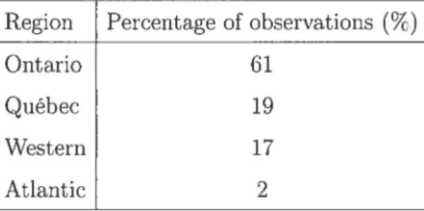
As we explained ahove, the analysis is donc on the Direct Market clients and prospects in the four regions of Canada using 2005 data. It is interesting to see how this population is distributed arnong the four regions of Canada. Table 1.1 shows that the majority of the Direct Market portfolio is in the province of Ontario. There is a sirnilar number of observations in the regions of Québec and

Western and a small number in the region of Atlantic.

TAB. 1.1. Direct Market population distributed by region in 2005. Region Percentage of observations (Y)

Ontario 61

Québec 19

Western 17

13

1.4.1. Descriptive analysis for Ontario

Since the majority of the Direct Market clients and prospects are in the

province of Ontario, the descriptive analysis is presented for this province only.

The data set includes 153.02$ clients and prospects in Ontario and 34 vari ables. However, only the most significant variables are described.

1.4.1.1. Dernographic variables

The demographic variables are variables that descrihe the individuals without regard to their automobile or residential information. Consequently. these vari ables are available for all the observations in the data set. Table 1.2 shows that there is an important majority of males in the population and that clients and prospects are alrnost equally represented.

TAB. 1.2. Percentages of observations for the variables gender? and ‘dllents for the province of Ontario in 2005.

Characteristic Percentage of observations (c)

Male 72

Client 46

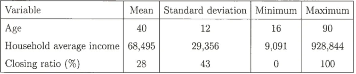
For the continuons variables, some descriptive statistics are presented in Table 1.3. The average age is around 40 and 28 of the population buys an insurance product. Furthermore, the distribution of the variable !age is represented in Figure 1.1.

1.4.1.2. Automobile variables

This subsection describes auto characteristics for individuals with at least one auto policy (clients) or who asked for an auto quote (prospect). In Ontario. 89% of the Direct Market population in 2005 had this characteristic. The 11% left are individuals that have only residential products. Table 1.4 shows the automobile

14 TAu. 1.3. Descriptive statistics for continuons demographic vari ables for the province of Ontario in 2005.

Variable Mean Standard deviation Minimum Maximum

Age 40 12 16 90

Household average income 68,495 29.356 9,091 928,844

Closing ratio

(%)

FIG. 1.1. Histogram of the variable “age.

characteristics for this subpopulation. For example, among the 89%, 65% of the individuals have or asks for collision protection. Note that the sum of all the percentages is not equal to 100% hecause a client or a prospect eau have more than one of these characteristics. For instance. a client may have a moto vehicle and a collision protection on his vehicle.

o — ,—.

15 TAB. 1.4. Percentages of observations with each auto characteristic for the province of Ontario in 2005.

Characteristic Percentage of observations (c)

Collision protection 65

Private passenger vehicle 88

Snowmohile vehicle 9

Moto vehicle 3

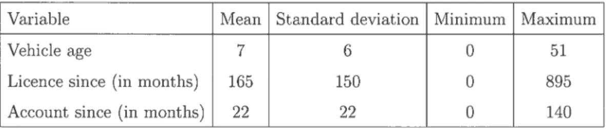
Table 1.5 presents other auto characteristics. These continuous variables are based on time notion and they ail have a minimum value of 0. For example, the minimum of O for the vehicie age means that the vehicie was new at the moment of the creation of the data set.

TAB. 1.5. Descriptive statistics for continuous variables related to auto policy for Ontario.

Variable Mean Standard deviation Minimum Maximum

Vehicle age 7 6 0 51

Licence since (in months) 165 150 0 895

Account since (in months) 22 22 0 140

1.4.1.3. Residentiat variabÏes

The characteristics described in this subsection are for individuais with at ieast one residential policy (clients) or who asked for a residential policy (prospect). In Ontario, 25c of the Direct Market population in 2005 had this characteristic. The75%’c left are individuals that have only automobile products. In Table 1.6, we sec that among the 25c, 69c of the observations have or asked for a homeowner package.

16 TAn. 1.6. Percentages of observations with each characteristic in Ontario.

Charact eristic Percent age of observations

₍

Homeowner package 69

Condo package 12

Tenant package 19

1.4.2. Average closing ratio

b model the closing ratio. only individuals who made a quote are included in the database. Indeed when the number of quotes is nuil. the closing ratio is missing. Consequently. the number of observations in the database is reduced 50

that each person has a value for the closing ratio. Table 1.7 shows the number of observations in each region with the corresponding closing ratio.

TAn. 1.7. Number of observations and closing ratio for each region.

Region Number of observations Closing ratio (c)

Ontario 105,635 2$

Québec 43,791 15

Western 31,666 25

Atiantic 4,074 27

In Table 1.7, we see that the regions of Ontario. Western and Atiantic have a similar closing ratio compared to Québec which has the smallest among the different regions. This is hecause the Québec market is more competitive and it is not as inuch regulated as the other provinces.

1.5.

EM

This section explains the EIvI algorithm that is used later in this pro.ject. In

our context, this algorithm is used to estimate the parameters of a mixture model. Furthermore. as we will sec in Chapter 3, the mixtures used here are mixtures of only two distributions.

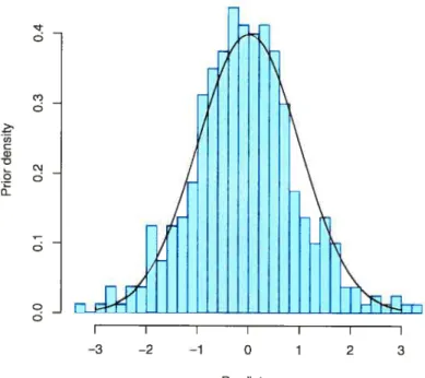
17 Suppose that the graphie representation of a variable is given hy the Figure 1.2. This bimodal graphie indicates that the variable lias a mixture distribution.

as 0 C G) o c\j

Fia. 1.2. Density of a mixture of two normal variables.

We eau define the random variable Y having a mixture of two distributions

Yl

Y2

Y=(1-A)Y1+AY2,

where L\ {O, 1} with IP(A = 1) _{= y. The density of y is therefore}

f(y) = (1 —p)øe1(y)+pg,(y).

where p is the prohability that an observation follows the distribution e5o2.

b estimate the parameters p. 6 and &2. the log-likelihood is calculat.ed as:

Ï(O;Z) log[(1 p)g1(yj)+p9(yj)].

o o I I I I I I 0 1 2 3 4 5 Y i=i

18

To maxirnize 1(0: Z). an iterative method is used and manv iterations are

required before convergence. In this Masters thesis. R proiect was used to execute

these iteratiolls. The algorithm is:

(1) take initial values for the parameters p. 01 aiid 02.

(2) compute the responsihilities:

- —

___________________

— (1 _{—p»ojy) +p62(yi)’} (3) generate u ‘- Bernouilli((),

(4) minimize the log-likelihood versus 0 and 02:

Ïo(O; Z. u) = {(1

— îi) log1 (y) + u 1ogg2(y)] + [(l

— u) log + u log]. where _{= r}

_Z

(5) Iterate steps 2 to 4 bv replacing 61 bv

_§.

A way to choose the initial values of 0 and 02 is to take two y at random. for

the parameter p. the initial value eau be anv value betweeu O and 1. In this Masters thesis, a value of 0.5 was choseu for this initial parameter (see Hastie et

aL. 2001).

This chapter began with the presentation of the two aims of the project. Also, it. presented the variables included in the database. Then, the variables explained in Section 1.3 were used to describe the Direct Market population and to construct a moUd that predict the closing ratio. Chapter 2 will explain two classic statistical methods to resolve the two objectives.

Chapter

2

CLA$$ICAL APPROACH

In Cliapter 1, the data set used for this project lias heen presented. This chapter descrihes two statistical methods applied to analyze these data. The main objec tive of this project is to predict who in the Direct Market segment is more likely to buy insurance products. However. in order to create statistical models. the understanding of the population under consideration is essential. Therefore, this chapter begins with the description of an exploratory data analysis method. In deed, Section 2.1 discusses about clustering. a statistical method to explore and to classify the data. In order to describe Direct Market clients and prospects, this technique tries to form homogeneous sub-groups which are very diffrent from each other. In this first section. the closing ratio is not yet modeled hecause the clustering is a descriptive method, i.e. a method that does not need a target variable.

Once the population of interest lias been studied, the objective is tofilld which individuals are more likely to huy insurance products. Hence, a statistical model must be developed to find these individuals. Therefore, some decision trees are constructed using the closing ratio as target variable. This is described in Section 2.2.

2.1. CLUsTERING

An objective of this project is getting to know a particular segment of Me-loche Monnex prospects and clients that is. tlie direct rnarket. However, because

20 the population in this segment is composed of the general public, many different individuals are in it. The population is thus an heterogeneous population. There fore, describing it glohally could be misleading. The cluster analysis answers this problem. This method lias the purpose of grouping clients and prospects into groups or clusters hased on similarity in their characteristics.

This section begins with the description and the definition of the cluster anal ysis. Then. we discuss the data preparation in Section 2.1.2. Afterward, sorne similarity and distance measures are presented in Sections 2.1.3 and 2.1.4. We follow in Section 2.1.5 with the explanation of two clustering strategies: the Hi erarchical clustering and the Partitional clustering. To conclude this section, we elahorate about the method used to find the optimal number of clusters.

2.1.1. Description

Cluster analysis is a common technique in exploratory data analysis. It is the classification of objects into different groups. More precisely. the data set is separated into subsets or clusters, so that all the objects in cadi cluster tend to be similar to cadi other. There is many way to cluster a data set. Therefore, the underlying mathematics of most of these methods are relatively simple but large numbers of calculations are needed.

Definition 2.1.1 (Cluster). A ctuster is a group of contiguous eternents of a statisticat poputation; for exampte, a group of peopte living in a singÏe house, a consecutive mn of observations in an ordered series, or a set of adjacent plots in one part of a field (cf. Everitt, 1993).

Definition 2.1.2 (Good clusters). Good ctusters are clusters that present Ïittte varzaton into the groups and large variation between the groups. They aÏso need to be large enough to be signiftcant.

21

We begin with an example of a data set that could be divided into clusters.

Example 2.1.1. This simulated data set is cornposed of 10 individuals with the foïlowing characteristics: their age. their number of auto daims and their ciosing ratio. It is represented in Tabte 2.1. The ciuster analysis is donc using “age” and “number of auto daims“. If an observation does not have any auto poticy, its number of auto daim is missing _{(“. “).} With this dataset, it is possible to group some similar individuats and produce 2 differents ciusters. One group couÏd inctude young persons with many auto daims whiÏe the other comttd be formed of older individuats with a smaÏter number of daims.

TAu. 2.1. DataofExample2.1.1.

Observations Age Number of auto daims Clos ing ratio

1 30 0 1.00 2 2 1 0.30 3 20 2 0.75 28 3 0.00 5 55 1 0.30 6 33 0.0 7 35 3 0.0 8 30 5 0.0 9 . 0.00 10 51 . 0.25

2.1.2. Preparing the data

Ina large database with many variables, the data must be preprocessed before they are analyzed. First of ail. the missing values must be examined carefully. Indeed, missing values eau have different meanings dependingon the variable. As we explained in Chapter 1, the variables eau be demographie. automobile or resi dential. For the demographie variables, the data set is eleaned in order to obtain

22 no missing value. For the auto variables. we must oniy have missing values for individuals without an auto po1icy The same principle is applied to residential variables while missing values must he for individuals without residential policy.

Another important consideration is the variable variances. For example. in the data set, some variables are expressed in thousands while others are in hun dreds. Therefore. variables with large variances tend to have more effect on the resulting clusters than variables with srnall variances. It is thus recommended to standardize these variables. However, if ail variables are measured in the same units. there is no need for standardization.

Definition 2.1.3 (standardization). A variable x is standardized wken its vat nes are transformed and given by:

[cii —

where is the mean ofx and uj, his standard deviation. 2.1.3. Similarity measure between individuals

A clustering method attempts to group the objects based on some measures of similarity. $imilarities are a set of rules that serve as criteria for grouping or separating items. It is possible to measure similarity and dissimilarity in a num ber of ways. Consequently there is not a single correct classification. In order to measure the sirnilarity, an important concept is the similarity matrix. This matrix represents the sirnilarities or the dissimilarities between the individuals present in the data set. It is used for the clustering algorithms. Therefore, we note D, the similarity matrix that is a n x n matrix where n is the number of observations. Each element of this matrix, noted dt is the similarity between the 1th _{and the} /th _{observation. This matrix is also symmetric and the diagonal elements are null.}

To compute the matrix D. a similarity measure must be specified. Thus, it is more common to measure the similarity as the dissimilarity between ob jects. Therefore, we define x r the predictor variables and d(x, xi), the

23 dissimilarity measure between ijj and xji, the values of the predictor i for the

observations

j

j’.

j

j’

j

j’

many different functions. These functions depends on the variable types that can he quantitative, ordinal or binary.

2.1.3.1. Similarity measure for quantitative variabtes

For the quantitative variables, we present the two most important measures:

(1) Euclidean distances: this is the most commonly chosen type of distance. It is the geometric distance in the multidimensional space. The distance between ij and is computed as:

,J(. . .

.1,3’) —

Ij L,3 an

D(x..rj,) ₌ d(i

(2) Manhattan distance: this distance is the average absolute value differ ence across dimensions.

— x’ and D(i,x) =

In Hastie et aï. (2001), a similarity measure based on the correlation between variables is described. In this case, the similarity measure is a similarity measure and is —

Z(x

Z

where Tj = 1 _{x is the average for the observation}

j

Another consideration is the distances measures for the ordinal variables. These variables are those where ah possible values are ranked depending on their importance. In that situation. the variables are transformed before the compu tation of the dissimilarity matrix. The measiire is given by (cf. Hastie et at.,

24 2001):

—

where ij is the value of the observation

j

and M is the number of categories for this variable. For each ordinal variable, this measure replaces the original one and the similarity matrix could be calculated using this transformed value. They are then treated as quantitative variables.

2.1.3.3. $irnitarity ‘rneasvre for binary variables

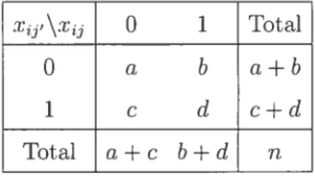
Many binary variables, also called dichotornous variables, are included in our data set. They categorize data in two groups with value O for one group and 1 for the other group. Suppose we observe the contingency table given in Table 2.2. where n is the number of observations.

TAB. 2.2. Values to calculate similarity measure for dichotomous variables.

xj\xj 0 1 Total

O a b a+b

1 e d c+d

Total a+c b+d n

Therefore, we can now define different dissimilarities measures (cf. Lorr. 1983). The usual dissimilarity functions are:

(1) d(x. = e±4 (Coefficient of coilcordance),

(2) d(;,it) — d Jacquard coefficient), — b+c+d — 2d (3) d(x, _j’) — 2d+b+c’ (4) d(x,

_.,)

—

—

_—

25 Now that some distances have been defined, the dissimilarities between x and

xj’ is given by:

D(.T.X) = d(x. xv),

where p is the number of predictor variables. Therefore. since the similarity matrix cari he determined, we have ail pairwise distances for the individuals.

2.1.4. Distance measure between clusters

Now that the similarity between ail individuals is determined, the distance between clusters cari he computed. However, hecause the clusters include many individuals. the distance hetween clusters is not easily calculated. Therefore, many distance functions exist. The usual measures to caiculate the distance between these two clusters are:

Centroid distance: the distance between groups is the distance between

the cluster centers called the group centroids. Therefore, in order to find the distance between two groups. let say H and L. the ciuster centers H

and mL must be determined. The centroid distance between these two

ciusters is:

jcentroid(H _{L) = rnH}

— mLL

where mH _Z=l Xi,’,. mL

Z=1 Z1

are the numbers of observations in groups H and L respectively.

This measure is flot appropriate when the sizes of the two clusters to be grouped are very different. In this case, the centroid of the new group will be very close to the centroid of the larger group. Thus. the properties of the smailer group are then virtually lost (cf. Everitt, 1993). However,

this measure has the advantage of only having to calculate the difference between each cluster centroid. In opposition, the three other distances described beiow need the calcuiation of the differences between every pairs of individuais in the two groups.

Single linkage clustering: this measure is also called “Minimum or Nearest

26 dissimilarity between members of the two clusters. that is

dsinrle(H _L) = min D(x,, xi).

XhH.x1L

This measure has the advantage of being the simplest but has the disad vantage that an outiier cari cause two groups of individuals to be clustered

when rnost of the individuals are really distant.

Complete linkage clustering: this measure is also called ‘Maximllm or Furthest-Neighhour I\/Iethod. The dissimilarity hetween 2 groups is equal to the greatest dissimilarity between a member of a given cluster and a member of the other one. This rnethod tends to produce very tight clusters of similar cases. The distance between clusters H and L is

dclee(H,_{L) max D(xj,,It).}

XhrH.x, L

Complete linkage has the advantage over single linkage in that within a cluster, all pairs of individuals will he within the distance at which the cluster was formed.

Group Average Method: the distance hetween groups is the average of the distances between pairs of individuals in the two groups. that is. the distance hetween clusters H and L is:

fil L

D(x1,xt).

Ft=1 t=1

This measure is a good compromise between the extremes of single and complete linkage. but the distances at which clusters are formed are av erages, not real distances. Therefore, the clusters can he more difficuit to interpret. However, it takes longer to evaluate.

2.1.5. Clustering strategies

Two main clustering strategies are discussed in this chapter: (1) hierarchical clustering,

27 (2) partitional clustering.

2.1.5.1. HieTaTchicat ctustering

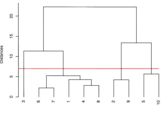
In hierarchical clustering, the data set is not partitioned into a partidular cluster. Instead, a series of partitions or merges take place, which may run from a single cluster containing ail ohjects to n clusters each containing a single ohject or the other way around. that is from n clusters to 1. Hierarchical clustering techniques are subdivided into top-down and hottom-up methods. A top-down method begins with ail observations in the same cluster. This cluster is gradually broken down into srnaller and smaller clusters. Bottorn-up techniques are more commonly used. Initially. each obj cet is assigned to its own cluster and then the algorithm proceeds iteratively. At each stage. the two most similar clusters are joined and it continues until there is just a single cluster. Therefore, the single observations are the smaller clusters possible. Hierarchical clustering may be represented by a two dirnensional diagram known as a dendrogram (see figure 2.2) which illustrates the fusions or divisions made at each successive stage of the analysis.

Definition 2.1.4 (Dendrogram). A dendrogram is a tree diagramfreqnentty nsed to itÏustrate the arrangement of the clnsters produced by a clnstering aÏgorithm.

The vertical axis represents the distances between ctusters and the horizontal axis is the observation sequence numbers. Each vertical tine represents a cluster.

Hierarchical clustering (sec section 2.1.5.1) was applied to Example 2.1.1. figure 2.1 shows three dendrograms using Euclidean distance and three distance measures hetween clusters. Although the distances hetween clusters are different, it is possible to sec that the merges are similar for ah measures.

The process of bottom-up hierarchical clustering can be summarized as fol lows:

(1) calculate the distance between ail initial clusters. In most analysis. initial clusters will be made up of individual cases,

28

Group Average Method Centroid distance Single Iinkage

w w

= C

ô ô

D O N— . ‘1 0 ni O U) O

f1G. 2.1. Dendrogram produced by hierarchical clustering on Ex

ample 2.1.1 using Euclidean distance and three distance measures. The final clusters are similar for the three distance methods.

(2) merge the two most similar clusters and recalculate the distances. (3) repeat step 2 until ail cases are in the same cluster.

The data set presented in Example 2.1.1 cari be classified using hottom-up clustering (sec Figure 2.2). It is possible to sec that the clustering algorithm begins with each observation being a single cluster. Then, we sec that individuals 6 and 7 are similar so they are grouped together. Table 2.3 shows the nine merging steps. Thus. at step 7, there is three clusters formed with (1, 3. 4. 6. 7. 8).(2, 9) and (5. 10).

In order to choose the final clusters. the dendrogram is used. Therefore. this representation shows the distance between the merged clusters. The more this

O O O ni O O w C O O O O ni

29 C c»J ID U) w Q C cI C U) ‘

I

f

FIG. 2.2. Dendrogram produced hy hierarchical clustering using Euclidean distance and group average method. It shows the dif ferent cluster merges. At the beginning. each observation forms a single cluster. Then, the observations are grouped until there is just one cluster. A visual inspection is used to choose the number of clusters by cutting the dendrogram at the desired level. The red une represents the eut off distance where the merges are stopped.

distance is important, the more clusters are different from another. As the dus ters are merged, the distances between them increase until the clusters are too dissimilar. At this moment, the clusters must stay distinct and the merging pro cess stops. Thus, an horizontal une is drawn in the dendrogram at this distance. The number of vertical unes that cross the horizontal line corresponds to the correct number of clusters. In Figure 2.2, the red line shows that there are four

ID

30 TAB. 2.3.

pie 2.1.1.

Merging process of the hierarchicai ciustering in Exam

Steps Clusters 1 (1).(2).(3).(4).(5).(6.7).(8).(9).(10) 2 (1).(2),(3),(4,8),(5).(6.7).(9).(10) 3 (1.4.8).(2).(3),(5).(6.7).(9).(10) 4 (1,4.8).(2.9).(3).(5),(6,7).(10) 5 (1,4,6,7,8) ,(2,9) ,(3) ,(5) ,(10) 6 (1.4.6.7.8).(2.9).(3).(5.10) 7 (1,3,4.6.7.8).(2.9).(5,10) 8 (1,3,4.6,7,8).(2.9.5.10) 9 (1.3.4.6,7,8.2.9.5.10)

different clusters. The observation 3 forms a single ciuster, the second inciudes (1, 4, 6. 7, 8), and the clusters 3 and 4 are respectively formed with (2, 9) and (5. 10).

In hierarchicai ciustering, there is a particuiar merging method calied \Vards classification. According to Ward (1963), the loss of information which resuits from grouping two ciusters can be measured by the total sum 0f squared devi

atiolls. At each step, the union of every possible pair of clusters is considered and the two ciusters whose fusion resuits in the minimum increase in the error of squares are combined (Everitt. 1993).

Hierarchical clustering is easily caicuiated but it is not adapted for large data sets. Furthermore, it does lot ahow provision for realiocation of entities who may have been poorly ciassified at an early stage in the analysis.

2.1.5.2. Fartitional ctnstering witk K-means ctustering

Partitional clustering is a ciustering method that directly divides the data set into clusters. The clustering algorithm optimizes a criterion function hased on two restrictions. It must minimize some measure of dissimilarity within the clusters and must maximize the dissimilarity between the different clusters.

31 Xz QOQ

o

ç.

e

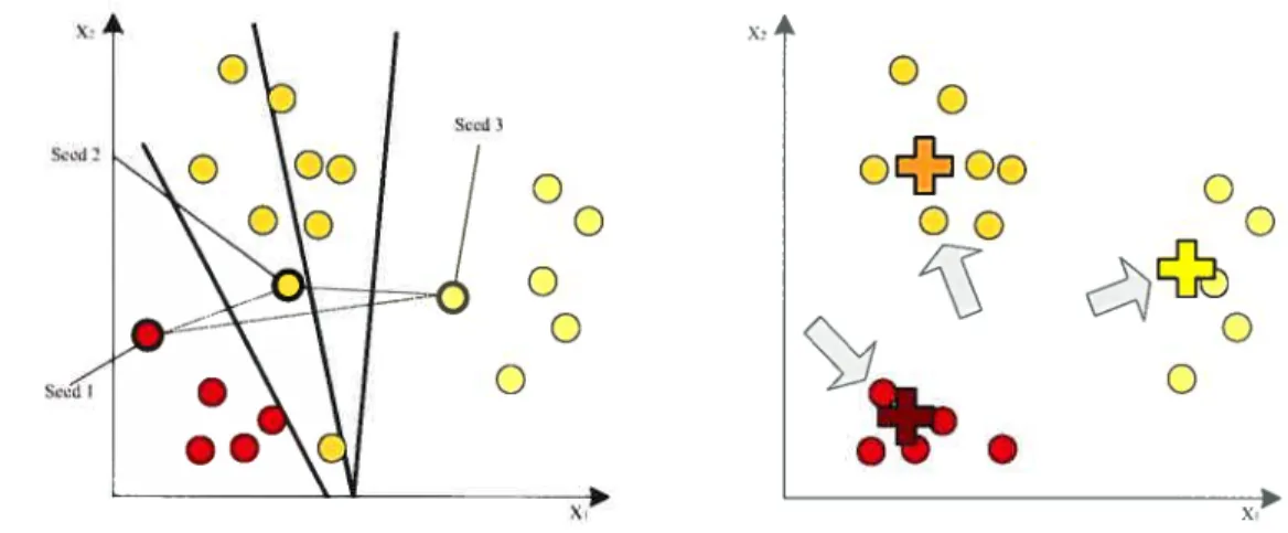
FIG. 2.3. Illustration of the K-means algorithm.

Partitional clustering differs from hierarchical clustering in that they admit relocation of the observations. Therefore, a poor classification might he corrected at a later stage. Hence. this is the chosen method for this project hecause it is appropriate for the efficient representation alld compression of large datahases. The partitional technique presented here is called the K-means method because it forms K different clusters. This method assumes that the number of groups has been decided a priori. The algorithm works as follow:

(1) randomly selects K seeds used as initial estimates of cluster centers. Many initialization methods eau be used. For example, MacQueen (1967): chooses the first K points in the sample as the initial cluster mean vectors. (2) Assign each record to its closest cluster center.

(3) Compute new cluster centers as the centroids of the clusters. (4) For each observation, calculate its distance from each centroid. (5) Repeat step 2 to 4 until convergence.

This algorithm is guaranteed to converge (see Andersberg. 1973). Seed 2

o

o

o

o

o

32 2.1.6. Number of clusters in K-means

One of the most important problem of cluster analysis is to identify the opti mum number of clusters. Consequently, many rnethods have been developed to determine this number.

Caliiiski and Harabasz (1974) developed a ratio given hy:

— (n

— K)trace(B$S) ratio

— — 1)trace(WSS)’

where n is the total number 0fobservations. K is the number of clusters. WSS is

the sum of squares within cluster, and BSS is the sum of squares between clusters.

Also. Duda and Hart(1973) proposed a criterion function that expresses how well a given K-cluster description matches the data. We expect a description in terms of K + 1 clusters to give a better fit than a description in term of K clusters. Therefore, to see if there is a statistically significant improvement in having K + 1 clusters instead of K clusters. the following ratio is computed:

WSS(K+1) ratio

WSS(K)

where 111S$(K+1) is the sum of squared errors within cluster when there is K+ 1 clusters and WSS(K) is the sum of squared errors within cluster when there is a K cluster. The nuil hypothesis that there are exactly K clusters is rejected at the d-percent significance level if:

WSS(K + 1)

<1 — 2 — /2(1 Sn2p)

WSS(K) irp

V

where p is the number of variables and cr is such as d = 1 — I(o.

Another criterion is proposed by Edwards and Cavalli-Sforza(1965). This ap proach minimizes the variability within groups as rneasured by the sum of the variation on each variable.

33 To estirnate the number of clusters. the chosen criterion for this project is the Cubic Clustering Criterion(CCC). This criterion is provided b the SAS pro gramming package (Sarle. 1983). 11 also minimizes the variahility within groups. We begin with some notations:

WSS: within-cluster sum of squares. ESS: error sum of squares.

n: number of observations in the data set. n:z_ _{number of observations in the kt1 cluster.}

p:rr rrnmber of variables,

K: number of clusters.

X : n z K matrix of variable observations,

X:

Z : n z p matrix of cluster indicator with elements Zjk for which:

f

Zjk = ‘Ç

O if otherwise.

Let. ZZt, a K z K diagonal matrix with the 0k on the diagonal and k = 1 K. such that

X=

The total-sample sum of squares and cross products (SSCP) matrix. denoted T

is given hy:

T = XtX.

The hetween-cluster $SCP niatrix BSS is:

BSS = ZtZ.

The within-cluster SSCP matrix is

WSS = (X — Z)’(X — Z)

= Xtx_X’zfz

34

The within-cluster sum of squares pooled over variables corresponds t.o the trace

of WSS. Since T is constant for a given sample. minimizing trace(WSS) is equivalent to maximizing:

R2 = 1

— trace(WSS)

(2.1.1)

trace(T)

where_{R2 is the proportion of variance accounted for by the clusters. The expeuted} value of R2. f(R2) is determined bv the assumption that the data have been

sampled from a uniform distribution based on a hyperbox. Therefore, in order to

obtain an approximation of E(R2). we have to find an approximation for R2 (cf

Sarle. 1983). The volume of the hyperbox. noted t’ is given bv:

‘L,

=

where s _{is the edge length of the hyperbox. If the hyperbox is divided into q} hvpercubes with edge length e. this length is given by:

c=(

The number of hypercubes along the dimension of the hyperbox is: si

=

Furthermore, we have that the total variance along theth _{dimension is propor}

tional to s2 and the within-cluster variance is proportional to e2. Therefore. R2

can he expressed by:

P 2

p2

— 1

______

ZPi=15j2

In Sarle (1983). the explain that the expected value E(R2). found with simula

tions is approximated by:

E(R2) =1

-fl+U fl+j (n

- q)2(1

+ (2.1.2)

Z=

35 The CCC is estimated from the observed R2 as:

ccc—i

1 — R2 (0.001 + E(R2))’•2

To estimate the number of clusters, the CCC is plotted against the number of clusters and the following conclusions can 5e made:

• the number of clusters that corresponds to maximums on the plot with the CCC > 2 or 3 is chosen and indicates good clustering.

• If there is a maximum with the C1CC between O and 2. there is possible clusters but t.hey should 5e int.erpreted cautiously.

• CCCis not appropriate for clusters that are highly elongated or irregularlv

shaped.

2.2.

In this section, a statistical model is developed to find the individuals who are insurance buvers. Therefore. some statistical models called CART are produced. CART stands for Classification and Regression Trees. As the name implies. the CART methodology involves using trees to resolve classification and regression proS leins.

This section starts with the description of the CART structure. Then. the method to construct the trees is explained in Section 2.2.2. To Setter understand this aspect, Section 2.2.3 explains the set of questions used to split the tree. Sec tion 2.2.4 discusses about some particularity of the data that affects the rnethod used for this analysis. In Section 2.2.5. the measures of goodness of spiit are pre sented and illustrated h means of an example. furthermore. to determine how large to grow the tree. two concept.s must be explained. Therefore. Section 2.2.6 explains the tree pruning and Section 2.2.7 describes the rules applied to stop the splitting. Once the trees are constructed, we want to know if they predict correctly the closing ratio. Thus, Section 2.2.8 presents how to evaluate these CART. This chapter is concluded with a discussion about the advantages and the disadvantage of the CART methodology.

36 2.2.1. Description

To predict the closing ratio, the statistical method used is the CART model. This technique allows us to find which groups are more likely to bu Meloche Monnex products hy partitioning the population into subgroups. A decision tree is a set of questions that spiits the data into subgroups depending on the value of the target variable. Consequentlv. we denote y. the target variable and X. the data set that include the vector of predictors .r = (Xi rp)t where p is the

fixed dimensionality. Therefore, the decision tree begins with ail data at the first node. also called the root node. from there, a spht criterion hased on a particular variable is used to divide the data set into suhgroups called the children nodes. For any node t. we suppose that there is a candidate split s” of variable .. However.

sorne definitions are needecl to better understand the decision tree structures. Definition 2.2.1 (Node). A node t is o partition ofthe dota set. If it is divided into chiÏdren nodes and if is catÏed a parent node.

Definitiori 2.2.2 (Root node). The root node is the comptete data set which

corresponds to flic top node ofthe free.

Definition 2.2.3 (Terminal node). A terminal node is a node with no children

nodes.

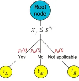
Some terminology must be given (see Figure 2.4):

tLt the Ieft chiidren node. tj: the rniddle chiidren node, tR: the right children node.

The proportions of the observations in the different children nodes of the parent node t are given by:

pL(t): proportion in t that goes into tL,

pM(t): proportion in t that goes into t1,

37 Figure 2.4 shows the CART structure. The root node is at the top of the

tree and there is three chiidren nodes with the corresponding prohabilities. In this example. because the chiidren nodes are not splitted. they are also terminal nodes.

PI

(t(t\PR(t)

Yes No Not applicable

FIG. _{2.4. Representation of the C1ART moclel. The root node is} divided into three chiidren nodes denoted tL. ti and 1R

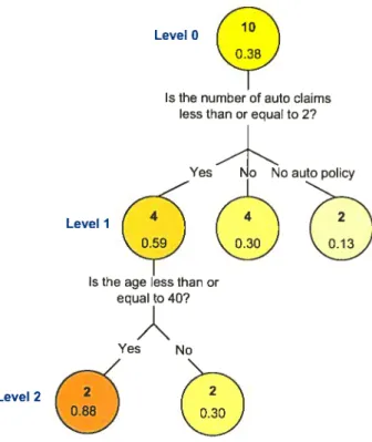
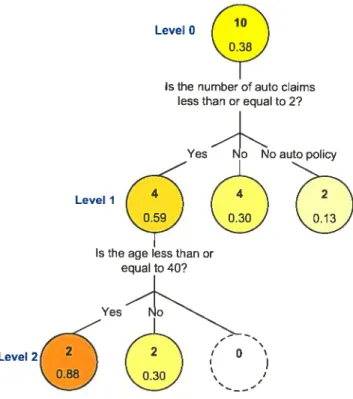
An important issue in the tree procedure is how to read a tree. The Example 2.1.1 cari he used to produce a tree. Figure 2.5 represents a tree that include two split questions. At the beginning, the 10 observations are in the root node and the average closing ratio is 0.38. The first spiit is produced bv the number of auto daims. The 4 observations with less than 2 auto daims are put in the left child node and have an average closing ratio of 0.59. The 4 observations with more than 2 auto daims are in the middle node and have a less important average closing ratio of 0.30. The right child node includes the 2 individuals without an auto policy and with an average closing ratio of 0.13 which is the lowest among the nodes. We ilote that their closing ratio is ouï for the residential part. At this point. the middle and the right child noUes are not divided. C1onsequently. these two nodes are terminal nodes. However. the left noUe is splitted with the variable

38 “age”. Therefore. the observations younger than 10 go in the left node and the others are put in the right node. We can see that this tree allowed us to find a group with a rnuch greater closing ratio than the average population. Indeed. the group with less than 2 auto daims and younger than 40 has an average closing ratio of 0.88.

Level O

s the number of auto daims less than or equal to 2?

Yes o auto policy

Level 1

Is the age less than or equal to 40?

À

Yes No

Level 2

FIG. 2.5. Example 2.1.1: tree model on 10 observations with the variables “age” and “number of daims”. Within each node. the flrst number is the number of observations present and the second corresponds to the average closing ratio. The clarker are the nodes. the greater is the average closing ratio within it.

In this chapter, we present the rnethod for CART models for the target vari able as a hinary variable. Hence, we consider a decision rule (presented in Chapter 3. Section 3.8) that assign O for individuals with a small closing ratio. and 1 oth erwise. Therefore. we are in a context of a two-categories t.arget variable.

39 2.2.2. Construction

First of ail, the data used to create the model is divided into three groups: the training set (70%) to huild a set of Inodels, the test set (30%) to see how the model performs on unseen data.

An important notion in the construction 0f decision trees is the liomogeneity.

Definition 2.2.4 (Homogeneity). A node is homogeneous wken ait the obser

votions in if are from. the sarne category. In oui’ contexi, an hornoge’neous node witt be a node that inciudes alt buyers or ail individv.als that do not buy any in surance product.

At the heginning of the tree algorithm. ail data is included in the root node. At this point. the objective is to divide this node into chulciren nodes to obtain homogeneous groups in term of closing ratio. Then. a spiit criterion using a par ticular variable is used to spiit the data set. This criterion, also called the splitting rule, must he chosen to perform the best split. At each node the tree algorithm searches through the variables one by one. heginning with .r1 anci continuing up to .v. For each variable it finds the hest split. Then it compares thep hest single variable split.s and selects the best of the best. In the next step. one or more of these regions are split and this process is continued until some stopping mie is applied. We note x the variable chosen to split the node t and s is the spiit value to execute the split.

Definition 2.2.5 (Splitting rule). A sptiting Tute is a criterion that divides the

data and that is composed with two etements: the variable used to spiit. and flic spÏit-point to achieve flic best sptit.

Definition 2.2.6 (Stopping rule). A stopping mie is a spiitting rute that makes

40 11w construct ion of a tree revolves around these elements:

(1) the choice of the best variable to spiit the data. (2) the definition of a set of questions

_Q

(3) the selection of the spiits by evaluating the goodness of spiit for any spiit 8Xt _{of any node t.}

(4) the decision when to declare a node terminal or to continue to spiit,

(5) the assignrnent of each terminal node to a class.

2.2.3. Set of questions

The set

_Q

_Q

(1) each split depends on the value of only a single variable.

(2) for each ordered variablei.

_Q

(3) if x is categorical. t.aking values in A (ai aL). the questions are of

the form ‘Is .r of a subset of A T’.

2.2.4. Data considerations for the spiits

In the literature, decision trees are binary, i.e. each parent node produces two chilciren nodes. Hastie et aL(2001) suggests that binary spÏits are better he cause multiwa _{spiits fragment the data too quicklv. Therefore. the next level} could include insufficient data. However, in our context, the splits can not always be binarv Indeed. the observations in the data set are divided in three categories:

(1) individuals with auto products only. (2) individuals with residentiai products oniy. (3) individuals with both produets.

41 In Chapter 1. wesaw that the variables can he auto variables. residential variables or demographic variables. In the Example 2.1.1. the number of daims is an auto variable and the age is a demographic variable. If flic variable used f0 separate the parent node is an auto variable. the observations without auto products does not have a value for this variable. We thus say that the answer to the question is not applicable for these individuals. Therefore, they are put in the right children node. On the other hand, if the answer to the question is ‘yes for an observa-t ion. iobserva-t goes in observa-the lefobserva-t chiidren node ad if observa-the answer is no??. if goes in the miciclie node. However, if the splitting rule is formed with a demographic variable. the split is binary because everyone in the data set has a value for these variables.

As we will see in Chapter 4, most of the time, tertiary splits happen at the beginning of the tree. Indeed, after sorne splits, the individuals without auto or residential products are isolated. The decision tree produced in this analysis has some binary splits and some tertiary splits. It does not affect the tree quality because the data set is verv large and the majority of the splits are binary.

2.2.5. Goodness of spiit

When the splitting rule is chosen. the objective is to have maximum homo geneity within a node. In other words, we want the child nodes to be as Ipurel? as possible. Let the split s at each node t that makes immediate descendent nodes as Hpure? as possible. A pure node is an homogeneous node. i.e a node with all the patterns of the same category. Although. it is more convenient to define the impurity rather than the purity of a node.

Definition 2.2.7 (Goodness ofsplit). A goodness of sptit is afunction 5(sX, t) for any sptit s’ of any noUe t nsed to evaïnate

if