HAL Id: tel-01078299
https://pastel.archives-ouvertes.fr/tel-01078299
Submitted on 28 Oct 2014
HAL is a multi-disciplinary open access
archive for the deposit and dissemination of sci-entific research documents, whether they are pub-lished or not. The documents may come from teaching and research institutions in France or abroad, or from public or private research centers.
L’archive ouverte pluridisciplinaire HAL, est destinée au dépôt et à la diffusion de documents scientifiques de niveau recherche, publiés ou non, émanant des établissements d’enseignement et de recherche français ou étrangers, des laboratoires publics ou privés.
Louis Plissonneau
To cite this version:
Louis Plissonneau. Network tomography from an operator perspective. Other [cs.OH]. Télécom Paris-Tech, 2012. English. �NNT : 2012ENST0033�. �tel-01078299�
EDITE - ED 130
Doctorat ParisTech
T H È S E
pour obtenir le grade de docteur délivré par
TELECOM ParisTech
Spécialité “INFORMATIQUE et RESEAUX”
présentée et soutenue publiquement par
Louis PLISSONNEAU
le 9 juillet 2012
Network Tomography
from an Operator Perspective
Directeur de thèse: Prof. Ernst BIERSACK
Jury
M. Chadi BARAKAT,INRIA, Sophia Antipolis - France Rapporteur
M. Refik MOLVA,EURECOM, Sophia Antipolis - France Examinateur et Président
M. Matti Mikael SIEKKINEN,AALTO University, Aalto - Finlande Examinateur
M. Guillaume URVOY-KELLER,Laboratoire I3S, Sophia Antipolis - France Rapporteur
TELECOM ParisTech
Abstract
Network tomography is the study of a network’s traffic characteristics using measures. This subject has already been addressed by a whole community of researchers, espe-cially to answer the need for knowledge of residential Internet traffic that ISPs have to carry. One of the main aspects of the Internet is that it evolves very quickly, so that there is a never ending need for Internet measurements. In this work, we address the issue of residential Internet measure from two different perspectives: passive measurements and active measurements.
In the first part of this thesis, we passively collect and analyse statistics of residen-tial users’ connections spanning over a whole week. We use this data to update and deepen our knowledge of Internet residential traffic. Then, we use clustering methods to form groups of users according to the application they use. This shows how the vast majority of customers are now using the Internet mainly for Web browsing and watching video Streaming. This data is also used to evaluate new opportunities for managing the traffic of a local ADSL platform. As the main part of the traffic is video streaming, we use multiple snapshots of packet captures of this traffic over a period of many years to accurately understand its evolution. Moreover we analyse and correlate its perfor-mance, defined out of quality of service indicators, to the behavior of the users of this service.
In the second part of this thesis, we take advantage of this knowledge to design a new tool for actively probing the quality of experience of video streaming sites. We have modeled the playback of streaming videos so that we are able to figure out its quality as perceived by the users. With this tool, we can understand the impact of the video server selection and the DNS servers on the user’s perception of the video quality. Moreover the ability to perform the experiments on different ISPs allows us to further dig into the delivery policies of video streaming sites.
Résumé
Le domaine de la mesure des caractéristiques du trafic transitant sur un réseau a été largement traité par une vaste communauté de chercheurs, en premier lieu pour ré-pondre aux attentes des opérateurs fournisseurs d’accès à Internet. En effet, leur pre-mière préoccupation est de savoir quel type de trafic ils doivent transporter. Une des principales caractéristiques de l’Internet est qu’il évolue très vite, de sorte que le besoin de mesures du trafic grand public ne se tarit jamais. Dans ce travail, nous abordons la question de la mesure du trafic Internet grand public par deux perspectives différentes : les mesures passives et les mesures actives.
Dans la première partie de cette thèse, nous capturons et analysons passivement les statistiques des connections d’utilisateurs d’Internet durant plus d’une semaine. Nous utilisons ces données pour réviser et approfondir notre connaissance du trafic Inter-net résidentiel. Ensuite, nous utilisons des méthodes de regroupement pour créer des ensembles d’utilisateurs en fonctions des applications qu’ils utilisent. Nous apprenons donc qu’une vaste majorité des clients se connectent à Internet principalement pour surfer sur le Web et regarder des vidéos en streaming. Ces données nous servent aussi à évaluer de nouvelles possibilités de contrôler le trafic d’une plateforme ADSL. Comme la principale partie du trafic provient du vidéo streaming, nous prenons plusieurs instan-tanés de ce trafic avec des captures paquet durant une période de plusieurs années, ceci pour comprendre précisément l’évolution de ce trafic. De plus, nous analysons et relions la performance du vidéo streaming, définie par des indicateurs de qualité de service, au comportement des utilisateurs de ce service.
Dans la deuxième partie de cette thèse, nous tirons parti de cette connaissance pour concevoir une sonde active capable de mesurer la qualité d’expérience des sites de vidéo streaming. Nous avons modélisé la lecture des vidéos streaming pour pouvoir déterminer leur qualité telle qu’elle est perçue par les utilisateurs. Grâce à cet outil, nous pouvons comprendre l’impact de la sélection du serveur vidéo et du serveur DNS sur la perception de la qualité vidéo par l’utilisateur. De plus, la possibilité de réaliser des mesures depuis divers opérateurs, nous permet de détailler les politiques de distribution vidéo utilisées par les sites de streaming.
Acknowledgements
Tuez-les tous, Dieu reconnaîtra les siens.1 Arnaud Amaury
The first person PhD students traditionally thank is their supervisor. I have always thought the main reason to do this is that he is the one to authorise you to defend your thesis. At least in my case, the main reason is not this one but the gratitude for giving me2 good scientific habits, namely explore every bit of data and plot readable graphs.
With these two mottoes in mind, any research work becomes much easier. So I would like to thank Ernst for accepting taking me as his student.
In the specific case of a part-time PhD, the person giving you the possibility to undertake these studies comes next in the acknowledgements. Here again, this is not the reason why I would like to thank Jean-Pierre Paris. It’s because his exemplary nature and his technical expertise are the North Star I’ve been following.
All the managers I’ve had during this long lasting PhD have helped and motivated me a lot. Here, I would like to specially mention Jean-Laurent Costeux.
A lot of people have contributed directly or indirectly to this thesis. I would like to thank Marcin Pietrzyk, Guillaume Vu-Brugier, Taoufik En-Najjary, Mickaël Meulle, Parikshit Juluri, Guillaume Urvoy-Keller, Deep Medhi, Stevens Le Blond, Moritz Steiner, Simon Leinen and all the other contributors who have worked with me during this PhD. I also would like to thank all my colleagues in Orange who have helped me building a strong and useful (or pragmatic) technical knowledge in the domain of networking. Even though I was not there often, I would like to thank the staff in Eurécom, especially Gwenaëlle Le-Stir, for making the administrative tasks transparent and painless. As usual, the last word goes to the family. My family has been very supportive, motivat-ing and understandmotivat-ing. I would say that hearmotivat-ing your children say “So finally, you are really going to finish your thesis!” is the greatest scientific achievement ever.
1
Kill them all, God will know his own. – my translation
2more precisely: forcefully instilling
Contents
List of Figures xiii
List of Tables xv
1 Introduction 1
1.1 Network Measurement: Tomography . . . 1
1.2 ISP Motivation . . . 2
1.3 Organisation of the Thesis. . . 3
I Passive Measurements 5 2 Passive Measurements Context and Methods 7 2.1 Methods and Tools for Passive Measurements . . . 7
2.2 Contributions . . . 9
2.2.1 Analysis of one week of ADSL connections . . . 9
2.2.2 HTTP Video Streaming Performance . . . 9
2.3 Related Work . . . 10
2.3.1 Network Tomography . . . 10
2.3.2 Video Streaming Studies . . . 10
3 Analysis of one Week of ADSL Traffic 13 3.1 Data Collection . . . 13
3.2 Characteristics of the Residential Traffic . . . 15
3.2.1 Application Share . . . 16
3.2.2 Refined Application Distribution . . . 17
3.2.3 Streaming Analysis. . . 18
3.2.4 Facebook . . . 18
3.2.5 YouTube. . . 20
3.2.6 Volumes. . . 21
3.2.7 Users’ Sessions . . . 23
3.2.8 User’s Level Analysis . . . 25
3.2.9 Performance Analysis . . . 32
3.3 Clustering Analysis . . . 32
3.3.1 “Real” vs. “fake” usage. . . 33
3.3.2 Choice of clustering . . . 33
3.3.3 Impact of Timescale on the Clustering Analysis . . . 34
3.3.4 Conclusion of the Users Clustering Analysis. . . 38
3.4 Dimensioning . . . 39
3.4.2 P2P Rate Limit at Peak Hour for Heavy Hitters only. . . 41
3.4.3 Conclusion on Dimensioning . . . 43
4 HTTP Video Streaming Performance 45 4.1 Novelty of this Work . . . 46
4.2 Trace Characteristics . . . 47
4.3 HTTP Streaming Context . . . 49
4.3.1 Most Popular Video Sharing Sites . . . 49
4.3.2 Video Encoding Rate . . . 49
4.3.3 Domain Name System (DNS) . . . 50
4.3.4 Distribution of Traffic across ASes . . . 51
4.4 Flow Performance Indicators . . . 52
4.4.1 Round Trip Time . . . 52
4.4.2 Peak Rate. . . 53
4.4.3 Mean Flow Rates. . . 56
4.4.4 Loss Rate . . . 58
4.4.5 Methodology for Monitoring . . . 62
4.5 User Behavior Study . . . 63
4.5.1 Downloaded Duration . . . 63
4.5.2 Simple User Experience Metric . . . 65
4.5.3 How do Users watch Videos . . . 66
5 Conclusion of Part I 69 5.1 Conclusions on the Analysis of Week-long Connection Statistics . . . 69
5.2 Conclusions on the Performance of HTTP Video Streaming . . . 70
5.2.1 YouTube Architecture and Video Servers Selection . . . 70
5.2.2 DailyMotion Delivery Policy . . . 71
5.2.3 Users’ Viewing Behavior. . . 71
5.2.4 Next Steps on Utilising Passive Packet Traces to Understand Video Streaming Traffic . . . 71
II Active Measurements 73 6 Active Measurements Context and Challenges 75 6.1 Active Measurements of HTTP Video Streaming . . . 75
6.2 Related Work . . . 76
6.3 Contributions . . . 77
6.3.1 Main Results . . . 77
6.3.2 Novelty of our Work . . . 77
7 Impact of YouTube Delivery Policies on the User Experience 79 7.1 Methodology . . . 79 7.1.1 Tool Presentation. . . 80 7.1.2 Validation Process . . . 81 7.2 Datasets Details . . . 82 7.2.1 Volunteer Crawls . . . 82 7.2.2 Controlled Crawls . . . 82
7.2.3 Kansas City Crawls . . . 83
7.3 Results . . . 83
7.3.2 DNS impact . . . 87
7.3.3 Evaluation of QoE Approximation Techniques . . . 88
7.4 YouTube Infrastructure . . . 90
7.4.1 Datacenters sizes . . . 90
7.4.2 Redirections . . . 92
8 Conclusion of Part II 95 9 Conclusion 97 III French Summary 99 10 Introduction 101 10.1 Mesure du réseau Internet. . . 101
10.2 Le point de vue des opérateurs . . . 102
10.3 Organisation de la thèse . . . 102
11 Principales Contributions 105 11.1 Mesures Passives . . . 105
11.1.1 Analyse d’une semaine de trafic ADSL. . . 105
11.1.2 Analyse de la performance du vidéo Streaming . . . 111
11.2 Mesures Actives . . . 113
11.2.1 Outil d’évaluation de la qualité d’expérience . . . 114
11.2.2 Présentation des données collectées . . . 115
11.2.3 Résultats . . . 116
12 Conclusion 121
List of Figures
3.1 Evolution of stats captured on the probe on Lyon’s probe for the whole
week . . . 15
3.2 Evolution of TCP Volume captured on the probe (aggregated by minute) on Lyon’s probe on 5thJuly . . . 15
3.3 Evolution of Nb. of Users of Facebook over the week for Lyon’s Probe . . 20
3.4 RTT from BAS towards Facebook servers . . . 21
3.5 CDF of Throughput for YouTube Connections (>400 kB) . . . 21
3.6 Evolution of YouTube traffic over the week for Lyon’s probe. . . 22
3.7 Evolution of YouTube traffic per day . . . 22
3.8 Schema of session construction . . . 23
3.9 CDF of session durations for Lyon probe on 05/07 (only cnx > 1 sec) . . . 24
3.10 CDF of session durations for P2P and Streaming for Lyon probe on 05/07 (only cnx > 1 sec) . . . 24
3.11 CDF of session durations per hour for Lyon probe on 05/07 (only cnx > 1 sec) . . . 25
3.12 Stats for all Users on Lyon’s probe . . . 26
3.13 Heavy Hitter 1 . . . 28
3.14 Evolution of Upstream Volume over the week for Heavy Hitter 1 . . . 29
3.15 Heavy Hitter 2 . . . 29
3.16 Heavy Hitter 3 . . . 30
3.17 Heavy Hitter 4 . . . 31
3.18 Loss Rates for all Users on Lyon’s probe . . . 32
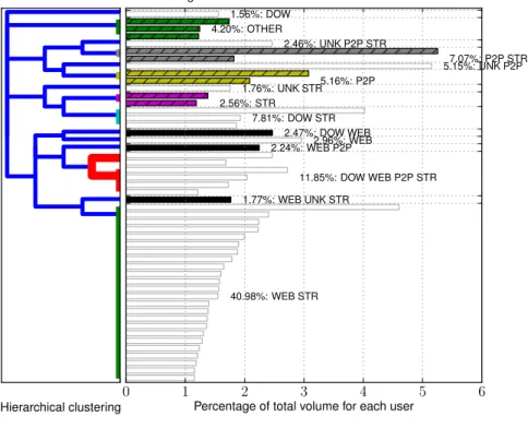
3.19 Clustering analysis for the whole week on Lyon’s probe . . . 36
3.20 Clustering analysis for the 12th(Tuesday) July on Lyon’s probe . . . 37
3.21 Clustering analysis for the 9thJuly (Saturday) on Lyon’s probe. . . 37
3.22 Clustering analysis per hour for the 5thJuly on Lyon’s probe at 8pm. . . . 38
3.23 Clustering analysis per hour for the 5thJuly on Lyon’s probe at 5pm. . . . 38
3.24 Evolution of the downstream Volume for the week on Lyon’s probe per application type . . . 39
3.25 Volume evolution on the platform for the week on Lyon’s probe . . . 40
3.26 CDF of the Throughput generated by the platform per hour on Tuesday 5thJuly . . . 41
3.27 CDF of the Throughput generated by 100 top users per hour on Tuesday 5thJuly . . . 42
3.28 Volume evolution on Tuesday 5th July on Lyon’s probe . . . 42
4.1 Internet seen by ISP Clients . . . 48
4.2 Video Encoding Rates for YouTube and DailyMotion . . . 49
4.3 RTT Computation Schema . . . 52
4.5 CDF of window sizes for FTTH M streaming flows. . . 54
4.6 Peak Rates per Flow . . . 54
4.7 YouTube Peak Rates per AS for the FTTH M 2009/12 trace . . . 55
4.8 Other Providers Peak Rates . . . 56
4.9 Mean Flow Rate of Videos for FTTH M traces . . . 56
4.10 Reception Rate of YouTube videos per serving AS for FTTH M 2010/11 trace . . . 58
4.11 Backbone Loss Rates . . . 59
4.12 Backbone Loss Rates per AS for YouTube videos on 2010/02 FTTH M trace . . . 60
4.13 Burstiness of Losses . . . 61
4.14 CDF of loss burstiness for YouTube FTTH M 2010/02 trace per AS . . . . 62
4.15 Monitoring Diagram: to apply to each streaming provider. . . 63
4.16 Fraction of Video Downloaded per Trace . . . 64
4.17 Percentage of downloaded volume for YouTube 2010/02 trace per AS . . 65
4.18 Fraction of Video Downloaded in function of Video Length for YouTube . . 67
4.19 Fraction of Video Downloaded as function of Video Reception Quality . . 67
4.20 Fraction of Video Downloaded as function of Video Reception Quality for Trace FTTH M 2010/02 for YouTube ASes . . . 68
7.1 Ping time in Milli-seconds to Main YouTube Cache Sites observed in a controlled crawl in December 2011 . . . 83
7.2 Evolution of the percentage of videos with at least one stall over Time (per period of 60 minutes) for two ISPs during December 2011 controlled crawl. . . 86
7.3 Ping Statistics differentiated by DNS for an ISP in Europe in May 2011 . . 88
7.4 Percentage of Redirection (over all videos) per YouTube Cache Site for ISP SFR-V4 per hour . . . 92
11.1 Analyse par regroupement des utilisateurs pour la semaine entière sur la sonde de Lyon . . . 110
11.2 Pourcentage de vidéo téléchargée en fonction de la durée de la vidéo pour YouTube . . . 112
11.3 Pourcentage de vidéo téléchargée en fonction de la qualité de réception . 113 11.4 Valeur du ping en milli-secondes vers les principaux sites de serveurs vidéo de YouTube observés dans une mesure contrôlée en décembre 2011 . . . 118
11.5 Évolution du pourcentage des vidéos avec au moins une interruption au cours du temps (par période de 60 minutes) pour 2 FAI dans une mesure contrôlée en décembre 2011 . . . 118
11.6 Carte indiquant la localisation des serveurs de vidéos, le nombre de requêtes obtenues sur chaque site (diamètre du cercle), et la distance (couleur du cercle : vert pour les ping ≤ 60 ms, bleu pour les ping ≥ 60 ms et ≤ 200 ms, et rouge pour les ping ≥ 200 ms) des sites de serveurs vidéos pour YouTube pour les mesures de Kansas-City (marque).. . . 120
List of Tables
3.1 Summary of Trace Details . . . 14
3.2 ... . . . 14
3.3 Distribution of Application Classes according to Downstream Volume per
Day and per Probe . . . 16
3.4 Distribution of Applications ordered by decreasing volume down for each class for Lyon’s probe over the week (from 05 to 12 July) only applications
with more than 1% vol down. . . 18
3.5 Composition of Streaming traffic over the week for Lyon’s probe (tables
are ranked according to decreasing downstream volume) . . . 19
3.6 Frequency of Connection for Facebook Users over the week for Lyon’s
probe . . . 19
3.7 Usage of Facebook (FB) for Lyon’s probe . . . 19
3.8 Distribution of Volume per Day (for Lyon probe) . . . 23
3.9 Distribution of Volume per Day (for Lyon probe) only Connections larger
than 1 kB in downstream . . . 23
3.10 Top 4 users (most up+down volume) week stats. . . 27
3.11 Ad-hoc, per application and user minimum hourly thresholds to declare
application usage . . . 33
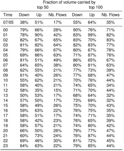
3.12 Fraction of Volume of top users . . . 35
4.1 Traces description . . . 47
4.2 Distribution of Volumes (in percent) and delays (median value of minimal
upstream RTT per flow) in milliseconds per AS for YouTube and DailyMotion 50
4.3 Distribution of number of distinct YouTube ASes per client for clients with
at least 4 YouTube videos . . . 51
4.4 Explanation of Loss Evaluation with downstream packets . . . 59
4.5 Fraction of Videos with Bad Reception Quality (normalized rate ≤ 1) . . . 65
7.1 Number of Videos for each ISP according to Regexp on Video Server Url
for a controlled crawl in December 2011 . . . 85
7.2 Ping times according to video server URLs for Kansas City crawls . . . . 86
7.3 Number of distinct IP addresses obtained with the 3 DNS servers (in
percent) . . . 88
7.4 Distribution of IP prefixes (/24) of video servers of all ISPs for controlled
crawls . . . 91
7.5 YouTube Datacenters sizes according to the Number of IP addresses
seen for crawls of all ISPs on each URL Regexp . . . 91
7.6 Percentage of Redirection per ISP for December 2011 controlled crawl . . 92
11.2 Répartition des classes d’application en fonction du volume descendant
par jour et par sonde . . . 107
11.3 Composition du trafic Streaming sur la semaine pour la sonde de Lyon
(les tableaux sont ordonnées en fonction du volume descendant) . . . 107
11.4 Seuils horaires par application et utilisateur pour déterminer l’usage
d’une application . . . 108
11.5 Pourcentage de Volume des top utilisateurs . . . 109
11.6 Top 4 utilisateurs (le plus de volume up+down) statistiques sur la semaine109
11.7 Description des traces . . . 111
11.8 Nombre de vidéos pour chaque FAI en fonction de Regexp sur les Urls
des serveurs vidéo pour une mesure contrôlée en décembre 2011 . . . . 117
11.9 Valeur de ping en fonction des sites de serveurs vidéos pour les mesures
C
HAPTER1
Introduction
Dessine-moi un mouton !1
Antoine de Saint-Exupéry, Le Petit Prince
1.1 Network Measurement: Tomography
Internet measurement can be undertaken at different levels: from an end-user computer to a router of the core network. The amount of data collected is thus a trade-off between the precision and the storage (or analysis) capacity of the system. A very coarse view of a system can be given by the count of the total amount of bytes or packets transiting through a network interface, this is a typical setup for routers transmitting Giga-Bytes of traffic per second. The most precise measurement is packet level trace and is usu-ally captured through dedicated software. The data measurement setup should not be determined by the capacity of the probe but by the precision of analysis required. The methodology of capture is as important as the data collection: actively requesting a server vs. passively duplicating Internet packets are two completely different methods that do not share the same objectives. Active probing can be used to measure how a service is accessed or what is its performance on a specific setup. On the contrary, passive measurements are usually taken at a much larger scale, but at the cost of losing the ability to customize the requests. Passive captures are used to understand what is actually happening on the monitored network.
The purpose of network tomography is not only to collect data, but to understand it. Usually, it imply evaluating the performance of an Internet connection. Internet perfor-mance can have many definitions depending on the point of view:
• at router scale, the drop rate of packets (independently of the connection) is the main indicator;
1Draw me a sheep – my translation
• on a transit link, the load of the link is of primary interest;
• for an ISP, the global load of a local platform determines not only the satisfaction of its customers, but also the need of upgrading the hardware;
• for a Web user, the delay encountered while accessing it favorite website is the only satisfaction measure;
• whereas a P2P user shall be mainly interested in the total throughput achieved for its file transfers;
• finally, a TCP expert can define the performance of a connection as the ratio of desequenced packets without retransmission only during bulk transfer periods. Here again the definition of performance should be taken according to the goal of the analysis and not to some pre-computed available metrics.
1.2 ISP Motivation
Internet Service Provider provide a so-called best-effort service: their first goal is to transmit packets between their customers and other machines on the Internet. Many factors have an impact on the customers connections:
• the access network capacity (and also collection infrastructure: ATM vs. GE); • the ISP network from the access collection point towards the destination of the
connection;
• the link capacity between the ISP and the next AS towards the destination; • the routing policies between all the ASes through which the packets will transit
until the destination.
Only some of these factors can be controlled by ISPs. Nevertheless, the main protocol used to transmit packets over the Internet is TCP which is an end-to-end protocol. This means that the packet analysis of a connection (at any point of measure) can give useful information on the path capacity and the resulting performance from the end-user point of view.
The motivation of an ISP is to give the best performance to its customers at a given cost (both for its own infrastructure and the peering agreements with other ASes). The use of different methods of measurement and analysis, as presented in this thesis, is thus of primary interest for ISPs. This can lead to new ways of managing the traffic ranging from local platform load management to TCP configuration according to the service accessed.
1.3 Organisation of the Thesis
The two main parts of the thesis are based on the choice of the measurement method: passive in PartIvs. active in PartII.
We first give the context and related work on passive measuring the Internet in Chap.2. The passive measurement studies in Part I benefits from data collected from many different sources and at very different scale. For Chap.3, we have analysed connection statistics over more than a week for 3 local ADSL platforms. This gives us many insights on the applications used2 and the performance of 4,000 different users. We also use
this information to evaluate innovative ways of managing a local platform. In Chap.4, we use multiple packet level traces of all users of a local ADSL platform during short time spans (1 hour) to focus on HTTP Streaming performance. This data has been collected over a period of three years. We show how the network conditions influence the behavior of users watching streaming videos. We conclude PartIin Chap.5. The challenges and related work on how to actively measure the Internet are given in Chap. 6. The active measurements presented in Chap. 7 have been collected by a new tool measuring the quality of experience of YouTube videos. We have collected data from many volunteers around the world, and also analysed data from a laboratory connected to the Internet through multiple ISPs. From this data, we figure out the main causes of perturbations of the end-user perceived quality. The main message is that link cost and ISP dependent policies have much more impact on the quality than usual quality of service metrics. Moreover, the access capacity on ADSL (and even more on FTTH) is no more a bottleneck in the access of video streaming service. We conclude PartIIin Chap.8.
Finally a conclusion of the thesis is given in Chap.9.
Passive Measurements
C
HAPTER2
Passive Measurements Context
and Methods
We don’t see things as they are, we see them as we are.
Anaïs Nin
Monitoring what is happening in a network (or on a link) without perturbing the traffic is of primary interest for an ISP. It gives the opportunity to understand and plan the development of the traffic transiting through its network. Nevertheless, if an operator would like to have a complete view of all its customers, the amount of data to capture can quickly become huge. Thus methods are used to reduce the data necessary to fit in the evolution of traffic. In this part, we focus on data collected from an ISP at a local platform level. We shall study in detail connection level statistics over a timescale of a week in Chap.3. This will give us an updated view of the actual traffic generated by residential users. We shall learn how streaming traffic (and especially video clips) is nowadays the main application in terms of downstream volume. In Chap.4, we use packet level traces during short timescale to precisely measure what is the performance of video streaming traffic and to determine the impact of the quality of service on the usage of video streaming.
In this chapter, we first recall main methods and tools used to passively capture Internet traffic in Sect.2.1. In Sect.2.2, we expose a summary of the main results of PartIand position our work in the passive measurements area. Finally, in Sect.2.3, we review relevant related work focusing particularly on video streaming as it is one of the main focus of this thesis.
2.1 Methods and Tools for Passive Measurements
The first method to monitor Internet traffic is to collect statistics on the border routers of the entity that would like to monitor its network. This is usually done through inquiry on SNMP counters of routers or switches. These measures are used to get a broad view
and no precise information can be expected from this data. Indeed, precise evaluation of the Internet traffic needs the concept of a connection (also called flow). Traffic monitoring literature defines a connection as an aggregation of packets identified by the same five tuple consisting of source and destination IP addresses, IP protocol, source and destination port numbers (for TCP and UDP only).
The next step towards precise measure of the traffic transiting through large routers is arguably Netflow records. Even though Netflow is originally a Cisco product, it is now recognised as a standard for traffic monitoring. Netflow records identify a connection as the standard five tuple plus the ingress interface and the IP type of service: this leads to unidirectional connections. Large routers give processing priority to the packet routing over the collection of Netflow records, thus random packet sampling was intro-duced in the collection process: only 1 packet out of n (usually n = 1000) is recorded. The accuracy and implication of this method has been studied in a large number of studies [31, 16, 11, 21, 7]. . . The main impact of this sampling is that it gives more importance to large flows (more likely to be caught by sampling) over small ones [12]. The large connections have been called elephants and small ones mice [6], and a whole taxonomy of Internet flows has thus been derived [9,5].
To overcome the limitation of packet sampling, many researchers have developed ded-icated probe to capture the Internet traffic The most popular packet capture softwares are tcpdump [52] and Wireshark [56]. They are based on the libpcap [32] C library, which is also the basis of many dedicated capture softwares (such as those devel-oped by ISPs). Even if in this thesis our passive capture tool is a private one, many other good software to passively capture Internet packet are freely available [54,50]. Dedicated hardware (such as Endace Dag cards [17]) can be used to cope with large amount of packets arriving at an interface, they also improve the precision of packet timestamping (which is useful to compute accurate performance indicators).
Once the question of how to capture has been resolved, the next question is: “Where to capture?” This is a crucial issue as the results drawn out of the measurements will highly depend on it. Many measurement studies are based on PlanetLab [38] or on Universities campuses (mainly in the US.). Even if modeling Internet connections can be done through this kind of measures, the lack of some applications (e.g. P2P, enterprise specific. . . ) induce a large bias in the results. For ISPs, it’s even more important to have data from residential customers, and this data has to come from a similar country (from geographic and linguistic point of view) to be transposable. The last question to address is: “What to capture?” Here again a trade-off has to be chosen between capturing more data for a shorter period of time, or having a long term analysis but reducing the scale of data captured.
Once we have collected data, the question of privacy arise. In the case of ISPs, we do not want (nor have the right to) divulge the contents of the packets transmitted. Nevertheless, if we take the analogy between a packet and a post letter, we focus only on the details given on the envelop (including TCP sequence number if needed) and not on the contents (the payload of a data packet). In the same problematic, anonymisation concerns have to be taken into account.
2.2 Contributions
In Part Iof the thesis, we use passive captures from residential customers in France. The data has been collected on a local platform aggregation point, namely at BAS (Broadband Access Server) level. We have used internally developed dedicated probes geographically distributed over France, and we have seen that the data is coherent between probes. This allows us to focus on a small number of different probes (three in Chap. 3, and two in Chap. 4). We analyse a week long of connection statistics in Chap. 3. This data offers a fresh view on what are the components of residential traffic nowadays. Whereas in Chap. 4, we take into account only Streaming traffic at packet level during snapshots of one hour. Nevertheless, we have performed multiple measurements campaigns that allows us to follow the evolution of Streaming traffic over a time span of three years.
2.2.1 Analysis of one week of ADSL connections
In Chap.3, we analyse the TCP traffic during one week of 3 ADSL platforms each con-necting more than 1,200 users to the Internet. We use connection statistics enhanced with a Deep Packet Inspection (DPI) tool to recognise the application. Top applications (Streaming, Web, Download and P2P) have the same volume and the same rank over days and probes in our data. The detail for each application is given, this gives us in-sights on what sub-class of application carries most of the bytes or the type of traffic generated. The ability to identify users allows us to follow their behavior independently of IP address churn, and the performance indicators helps us to better understand how the applications behave. The difference of traffic patterns between working days and week-end days is also studied.
The clustering analysis allows us to understand the application mix of users: the surge of plenty of customers using only Web and Streaming is quantified. Moreover, we explore the possibility to change the timescale of analysis. Our results shows that, if well chosen (namely during busy periods), a snapshot of one hour of traffic can be as representative as a whole week. Top 20 users (in terms of volume) have quite a specialized application mix, and their share of the platform load is about 10 times more than the average.
We also address the question of local platform dimensioning. We perform some sim-ulation to show how a well chosen rate limit policy could reduce peak rate at a very moderate impact for the users.
2.2.2 HTTP Video Streaming Performance
Chapter4 investigates HTTP streaming traffic from an ISP perspective. As streaming traffic now represents nearly half of the residential Internet traffic, understanding its characteristics is important. We focus on two major video sharing sites, YouTube and DailyMotion.
We use eight packet traces from a residential ISP network, four for ADSL and four for FTTH customers, captured between 2008 and 2010. Covering a time span of three years allows us to identify changes in the service infrastructure of some providers. From the packet traces, we infer for each streaming flow the video characteristics, such as duration and encoding rate, as well as TCP flow characteristics: minimum RTT, mean and peak download rates, and mean loss rate. Using additional information from the BGP routing tables allows us to identify the originating Autonomous System (AS). With this data, we can uncover: the server side distribution policy (e.g. mean or peak rate limitations), the impact of the serving AS on the flow characteristics and the impact of the reception quality on user behavior.
A unique aspect of our work is how to measure the reception quality of the video and its impact on the viewing behavior. We see that not even half of the videos are fully downloaded. For short videos of 3 minutes or less, users stop downloading at any point, while for videos longer than 3 minutes, users either stop downloading early on or fully download the video. When the reception quality deteriorates, fewer videos are fully downloaded, and the decision to interrupt download is taken earlier.
We conclude that
(i) the video sharing sites have a major control over the delivery of the video and its reception quality through DNS resolution and server side streaming policy,
(ii) that the server chosen to stream the video is often not the one that assures the best video reception quality.
2.3 Related Work
After a very brief review of passive measurements works, we focus on HTTP Streaming studies as most of our contributions focus on this traffic.
2.3.1 Network Tomography
Network tomography is a large domain and the relevant publications are numerous. The most authoritative reference is the “Internet Measurement” book [15]. Here are a very small number of works that have inspired us in the field of passive measurements: [35,
47,33].
2.3.2 Video Streaming Studies
Most related work on video sharing sites focuses on YouTube, which is the most promi-nent video sharing site. There is no previous work to compare YouTube with its com-petitors such as DailyMotion.
2.3.2.1 Characterisation of YouTube Videos
Many studies have tried to find out the characteristics of YouTube videos compared to e.g. Web traffic or traditional streaming video sites (real time over UDP and not PDL1). In [10], the authors crawled the YouTube video meta-information to derive many char-acteristics on the video contents and its evolution with video age (e.g. popularity). This information is used to evaluate opportunities of P2P distribution and caching.
In [13], the authors use a long term crawl of the YouTube site to derive global character-istics of YouTube videos such as that the links between related YouTube videos form a small-world network. Using the properties of this graph and the video size distribution, they show that P2P distribution needs to be specifically adapted to distribute YouTube videos.
In [25], the authors use university campus traffic to gather information on YouTube video characteristics and complement their data with a crawl of most popular files on YouTube. Temporal locality of videos and transfer characteristics are analyzed, and the opportu-nities for network providers and for service providers are studied. Another work of same authors [24] uses the same campus traces to characterize user sessions on YouTube showing that the think time and data transfered by YouTube users are actually longer than for Web traffic.
2.3.2.2 YouTube CDN Architecture
Some recent papers study the global architecture of the YouTube CDN2. In [2], the
authors explain with Tier-1 NetFlow statistics some of the load-balancing policies used by YouTube and use these measurements to figure out traffic dynamics outside the ISP network. This method is used to evaluate different load-balancing and routing policies. Even if the methodology still holds, the data collected for this work was taken before heavy changes in YouTube infrastructure in the second half of 2008 (two years after Google bought YouTube).
The same authors study the YouTube server selection strategy [3]. Using PlanetLab nodes to probe and measure YouTube video transfers, this analysis shows that YouTube is using many different cache servers hosted inside their network or by other ISPs. Some of the load-balancing techniques used by YouTube are also revealed in this paper. In the same vein, the authors of [53] use recent traces from different countries and access type (university campus vs. ADSL and FTTH on an ISP networks) to analyse the YouTube service policy. In most cases, YouTube selects a geographically close server except when these servers are heavily loaded.
The details of YouTube video streams at TCP level have been studied in [45]. This analysis of residential ISP datasets shows that the bursty nature of the YouTube video flow is responsible for most of the loss events seen. In [44], the interaction of the type of application and the type of video playback strategy with TCP is studied on Netflix and YouTube records. This shows how ON-OFF cycles can occur in video streaming
trans-1PDL: Progressive DownLoad
fers. Moreover a model of these behaviors is used to forecast the impact of expected changes (more mobile traffic, use of HTML5. . . ) on the network.
We also would like to mention this work on load-balancing in CDNs [42]. Here the answers of DNS queries towards CDNs are stored at ISP level in order to bypass recur-sive DNS resolution by the CDN. This allows to directly answer to the customers with an IP address chosen by the ISP instead of the CDN. The evaluation of this mechanism shows an improved performance, e.g. download time are reduced by up to a factor of four. This work shows that a cooperation between the CDN operators and the ISPs could not only be beneficial to these actors but also to the users. In a similar vein, the study of YouTube [53] also illustrates the importance of DNS resolution in server selec-tion and how video sharing sites (and more generally CDNs) use it to apply complex load-balancing strategies. Also the influence of traffic management between ISPs and main CDNs is underlined in [19].
C
HAPTER3
Analysis of one Week of ADSL
Traffic
Vous arrivez devant la nature avec des théories, la nature flanque tout par terre.1
Pierre-Auguste Renoir
The Internet is a very dynamic environment: new services and usages are invented every day. The attempt to measure it is thus an endless challenge. Nevertheless, regular measures are needed to quantify its evolution. The diversity of the Internet also resides in the ways to access it: of the many access types (from work, Universities, or home), residential access is the most free. Indeed no traffic regulation apply, and only few studies have revealed the residential usage of the Internet [55,36,33].
In this chapter, we perform a large scale analysis of 3 different local ADSL platforms each connecting more than 1,200 users during one week of July 2011. We use an inter-nal deep packet inspection (DPI) tool to recognise the application used by customers. With this information and connection summaries, we first study the characteristics of the residential traffic, and also focus on some specific popular services such as Facebook or YouTube. We then use clustering techniques to group customers according to their application mix. Finally, we simulate some traffic shaping techniques to evaluate their impact on platform dimensioning.
3.1 Data Collection
We have collected statistical information on 3 ADSL probes in France (located in Lyon, Montsouris and Rennes) over a period of one week of 2011: from Tuesday the 5thJuly to Tuesday the 12th July included. The data comprises information summary of the
1You come in front of nature full of theories, then nature messes everything. – my translation
Table 3.1: Summary of Trace Details
Nb of Clients Nb of Cnx
Trace Total Avg per Day Total Removed† Avg per Day
Lyon252 1354 1284 66,231,068 86,576 7,788,835
Mont151 1009 951 50,008,566 59,393 6,251,070
Renn257 1139 1099 41,320,018 35,847 5,165,002
†data cleaning as explained in Sect.3.1
name nr.
1 159
2 159
Table 3.2: ...
TCP connections of all customers for each day of capture2. The following indicators
have been computed for our analysis:
Cnx Id the source and destination IP addresses and Ports, and the time of start and
stop of connection;
Application determined out of an internally developed DPI tool, we have access to
the application, and also web-apps (such as Facebook) and a part of encrypted eMule and BitTorrent, still we shall mainly refer only to the class of the application (namely P2P, Streaming. . . );
Volumes the number of Bytes (with IP headers and also difference between last and
first TCP sequence number) and non-empty Packets for each direction of the connection, we will also use the maximum volume per period of 20 seconds;
TCP Performance we define the expected sequence number as the maximum TCP
sequence number seen plus the size of this packet, then a packet with a se-quence number higher than the expected one is counted as a loss, whereas if it’s lower, it’s counted as a repetition; we also have an evaluation of RTT. All these indicators are computed for each direction of the connection.
This data is complemented with specific HTTP streaming indicators with the URL and URI of the media, and a classification according to URL of well known sites (for adver-tisement, video clips, porn sites. . . ).
As this data is collected on the fly on probes connected to a switch after the BAS, we may have some incorrect records. Thus, we filter out the connections with incorrect statistics. The number of connections removed is included in Tab.3.1.
In all the rest of the Chapter (and of the thesis), we call downstream traffic the packets coming from the Internet to the customers, whereas upstream traffic denotes packets going from the customers to the Internet.
0 10000 20000 30000 40000 50000 60000 70000 80000 90000 Time in seconds 0 1 2 3 4 5 6 7 V ol um e (a gg re ga te d by 60 0 se cs .)
×109 Evolution of Volume for Lyon252 probe
07/05 07/06 07/07 07/08 07/09 07/10 07/11 07/12
(a) Volume (aggregated by 10 minutes)
0 10000 20000 30000 40000 50000 60000 70000 80000 90000 Time in seconds 900 950 1000 1050 1100 1150 1200 1250 N b of U se rs (a gg re ga te d by 36 00 se cs
.) Evolution of Nb of Users for Lyon252 probe
07/05 07/06 07/07 07/08 07/09 07/10 07/11 07/12
(b) Nb. of Users (aggregated by 1 hour)
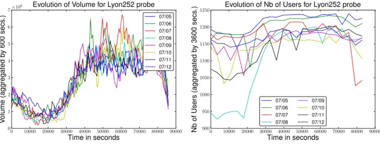
Figure 3.1: Evolution of stats captured on the probe on Lyon’s probe for the whole week
0 10000 20000 30000 40000 50000 60000 70000 80000 90000 Time in seconds 0 1 2 3 4 5 6 7 8 V ol um e in B yt es (a gg re ga te d by 60 se cs
.) ×108 Evolution of Volume for Lyon252 probe
07/07 (a) Thursday, 7th 0 10000 20000 30000 40000 50000 60000 70000 80000 90000 Time in seconds 0 1 2 3 4 5 6 7 V ol um e in B yt es (a gg re ga te d by 60 se cs
.) ×108 Evolution of Volume for Lyon252 probe
07/09
(b) Sunday, 9th
Figure 3.2: Evolution of TCP Volume captured on the probe (aggregated by minute) on Lyon’s
probe on 5thJuly
3.2 Basic Characteristics of the Residential Traffic
To give an overview of the data, we start by showing the evolution of volume and num-ber of users over the week, we plot each days on Fig. 3.1. The curve of the volume (Fig.3.1a) shows a very similar pattern over the week. Thursday the 7thhas the highest volume whereas Sunday the 9thhas the lowest. As for the number of users (Fig.3.1b), there are some differences between the days: for example, Saturday night has the least amount of users.
In Fig.3.2, we trace the evolution of volume (TCP) over two different days of the week. On a week day (Fig.3.2a), we observe an unsurprising camel curve with 2 large peaks around the mid-day break. Whereas on Sunday (Fig. 3.2b), we have a large plateau from late morning to early afternoon.
Table 3.3: Distribution of Application Classes according to Downstream Volume per Day and
per Probe
(a) Lyon
Top Applications (fraction of total downstream volume)
Date 1 2 3 4 5
05/07/2011 Streaming (47.69 %) Web (18.75 %) Download (18.13 %) P2P (8.49 %) Games (2.45 %)
06/07/2011 Streaming (47.95 %) Web (19.56 %) Download (17.29 %) P2P (9.25 %) Games (2.78 %)
07/07/2011 Streaming (47.79 %) Download (19.53 %) Web (18.22 %) P2P (10.26 %) Mail (1.66 %)
08/07/2011 Streaming (44.73 %) Download (21.40 %) Web (18.66 %) P2P (6.98 %) Games (3.48 %)
09/07/2011 Streaming (48.82 %) Download (21.67 %) Web (15.93 %) P2P (10.31 %) Unknown (1.60 %)
10/07/2011 Streaming (53.38 %) Download (17.90 %) Web (17.24 %) P2P (8.46 %) News (1.02 %)
11/07/2011 Streaming (49.01 %) Web (20.52 %) Download (15.93 %) P2P (9.52 %) Unknown (1.97 %)
12/07/2011 Streaming (51.64 %) Web (19.19 %) Download (14.29 %) P2P (9.78 %) Unknown (2.62 %)
(b) Montsouris
Top Applications (fraction of total downstream volume)
Date 1 2 3 4 5
05/07/2011 Streaming (38.86 %) Web (25.47 %) Download (21.37 %) P2P (7.81 %) Mail (3.18 %)
06/07/2011 Streaming (44.78 %) Web (22.48 %) Download (17.19 %) P2P (7.64 %) Mail (4.17 %)
07/07/2011 Streaming (43.26 %) Web (23.62 %) Download (18.67 %) P2P (6.28 %) Mail (3.84 %)
08/07/2011 Streaming (44.94 %) Web (22.99 %) Download (17.42 %) P2P (5.38 %) Mail (4.67 %)
09/07/2011 Streaming (48.70 %) Web (21.94 %) Download (15.70 %) P2P (7.42 %) Unknown (2.94 %)
10/07/2011 Streaming (48.21 %) Web (17.00 %) Download (16.42 %) P2P (13.64 %) Unknown (2.12 %)
11/07/2011 Streaming (42.76 %) Web (23.87 %) Download (20.79 %) P2P (5.65 %) Mail (4.19 %)
12/07/2011 Streaming (39.86 %) Download (24.96 %) Web (21.23 %) P2P (7.25 %) Mail (3.72 %)
(c) Rennes
Top Applications (fraction of total downstream volume)
Date 1 2 3 4 5
05/07/2011 Streaming (47.23 %) Download (24.07 %) Web (16.12 %) P2P (5.38 %) News (3.19 %)
06/07/2011 Streaming (46.35 %) Download (23.55 %) Web (15.93 %) P2P (7.74 %) Games (2.40 %)
07/07/2011 Streaming (47.34 %) Download (23.48 %) Web (16.43 %) P2P (7.80 %) Mail (1.73 %)
08/07/2011 Streaming (43.81 %) Download (26.73 %) Web (16.25 %) P2P (6.09 %) Enterprise (3.41 %)
09/07/2011 Streaming (44.21 %) Download (25.54 %) Web (15.53 %) P2P (8.56 %) Enterprise (3.19 %)
10/07/2011 Streaming (41.58 %) Download (22.86 %) Web (19.06 %) P2P (11.12 %) Games (2.60 %)
11/07/2011 Streaming (36.92 %) Download (19.52 %) Web (15.81 %) P2P (11.52 %) Unknown (6.29 %)
12/07/2011 Streaming (40.15 %) Download (19.92 %) Web (16.78 %) P2P (10.66 %) Unknown (5.03 %)
3.2.1 Application Share
We summarize in Tab. 3.3 the distribution of applications per number of connections and per volumes. Note that we consider only application classes.
In Tab. 3.3Streaming is by far the most used application in downstream volume. The next two application classes are Web and Download with very similar share of down-stream volume. The 4thmost popular application is P2P. The order is quite stable over the days or over the different locations. The downstream volume generated by all other application is very low (less than 10%) compared to the one of the top 4 application classes.
3.2.2 Refined Application Distribution
For the most popular application classes, we detail the repartition of applications over the week in Tab.3.4. We give the percentage of users, of flows, of volumes (down and up) for each application, and also the mean volumes (down and up) per flow. We have also computed the same statistics on application distribution over each day. As there is no notable difference in the weekly stats vs. daily stats, we do not include the daily data.
Table3.4gives us a finer view of the key components of the traffic. We first focus on the Streaming class. Here is the detail of Streaming applications in the table:
• HTTP-FLV and HTTP-MP4 are the main videos formats used by popular video streaming sharing sites (like YouTube);
• HTTP-STREAMING regroups other formats of videos (mainly used for small em-bedded advertisements);
• RTMP related protocols are usually used to deliver on demand video streaming (note that RTMPE is only used by a specific popular TV channel for its replay service: M6Replay).
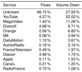
The HTTP-STREAMING class appears for almost all users, and represents 3/4 of flows. The mean downstream volume is very low as the durations of these ads videos are very small (a few seconds). In upstream, as the mean volume is almost the same for the main Streaming applications, the fraction of upstream volume generated by HTTP-STREAMING flows represents a large part of the total due to its huge number of flows. This table allows us to quantify that FLV is used about 4 times more than MP4. Indeed, this is the default format for YouTube which is the most popular video streaming site. As for Web traffic which is used by almost all users, the images on the Web sites carry most of the bytes of this class. We can note that secured Web transfers (with TLS or on 443 TCP port) are used by 4/5 of users, but it represents only 5% of flows. Finally, even if the fraction of flow and volume on Facebook is very low (less than 1% thus not in the table), two third of the clients use it.
The Download class is used by 9/10 users because of Web Downloads. Even though HTTP File Sharing is used by a small fraction of users (7%), it represents almost half of downstream volume. This is due to the large volume per flow (16 MBytes), and the most popular file sharing site at this time was MegaUpload.
P2P is used by about 10% of users and represents 10% of the total traffic (Tab.3.3). The information in Tab.3.4is very interesting to understand new trends in P2P networks:
• BitTorrent is the most popular P2P application, and even if its encrypted version is used by half of BitTorrent users, the total downstream volume that is encrypted is very low compared to non-encrypted one;
• eMule/eDonkey is the second most popular P2P application, but in this case the encrypted protocol is the most popular (both in terms of users and bytes);
Table 3.4: Distribution of Applications ordered by decreasing volume down for each class for
Lyon’s probe over the week (from 05 to 12 July) only applications with more than 1% vol down
Mean per Flow
App. Class App. Nb. Users Nb. Flows Vol. Down Vol. Up Vol. Down Vol. Up
Streaming HTTP-FLV 59.22 % 16.99 % 51.64 % 12.80 % 5 695 173,3 1 704,1 Streaming HTTP-STREAMING 93.42 % 74.50 % 32.71 % 60.16 % 822 918,7 1 827,7 Streaming RTMPE 4.57 % 0.17 % 6.05 % 0.34 % 68 066 027,7 4 588,0 Streaming RTMP-Data 20.12 % 0.94 % 3.49 % 10.22 % 6 951 763,4 24 538,5 Streaming HTTP-MP4 17.26 % 3.89 % 2.85 % 1.56 % 1 372 468,9 905,1 Streaming RTMP 13.10 % 0.50 % 1.17 % 4.07 % 4 394 348,0 18 427,4
Web Images Web 81.08 % 29.61 % 52.48 % 29.52 % 28 561,8 2 267,9
Web Default http 80 86.73 % 34.37 % 25.50 % 35.24 % 11 954,8 2 332,4 Web TLS 80.68 % 5.10 % 8.49 % 14.86 % 26 849,9 6 631,5 Web http 80.57 % 7.85 % 7.14 % 8.25 % 14 671,0 2 390,3 Web Unknown 99.89 % 20.09 % 3.42 % 6.76 % 2 742,6 765,5 Web Other443 49.64 % 1.04 % 1.81 % 0.25 % 28 122,5 550,1 Download DownloadWeb 88.20 % 52.34 % 46.57 % 9.44 % 558 654,8 1 796,6
Download HTTP File Sharing 6.95 % 1.81 % 45.53 % 1.00 % 15 785 114,3 5 485,5
Download AppStore 2.98 % 0.17 % 4.01 % 0.01 % 14 790 512,3 859,7 Download Encrypted FTP 2.82 % 0.20 % 1.98 % 7.84 % 6 262 936,5 393 622,5 Download FTP-Data-Passive 7.72 % 18.24 % 1.37 % 41.46 % 47 243,0 22 640,9 P2P Bittorrent 7.24 % 59.65 % 45.79 % 25.56 % 30 506,6 8 995,1 P2P eMuleEncrypted 4.68 % 3.11 % 28.53 % 43.74 % 364 595,6 295 240,0 P2P eDonkey 2.79 % 7.67 % 16.23 % 18.46 % 84 070,5 50 512,8 P2P BitTorrentEncrypted 4.34 % 0.60 % 8.33 % 9.58 % 552 204,8 335 471,8
• the ratio of downstream to upstream volume is 3 times higher for BitTorrent than for eMule/eDonkey (we cannot compute it in the table as the fraction of volumes are separated by direction and thus are not comparable).
3.2.3 Streaming Analysis
We focus in this section more closely on the composition of streaming traffic in Tab.3.5. The streaming traffic consists mainly of Clips if we consider downstream volume, see
Tab.3.5a. But Advertisement and Unknown (most probably advertisements) represent
the majority of flows. The categories are obtained through pattern matching on URLs with well-known services.
We can rank streaming sites in Tab. 3.5b according to their share of downstream vol-ume. Note that the upstream volume is very low for this application class. YouTube represents more than 1/5 of total downstream volume, and its next competitor gener-ates only half of its traffc (10%). Then comes porn sites and TV replay sites. Note that the most popular music streaming site represents 5% of flows (but a lower share of volume).
3.2.4 Facebook
We have seen in Sect.3.2.2that the fraction of users on Facebook is about 2/3 of users over the week. In Tab.3.6, we compute for each Facebook user how many days he has been connecting to the service. We learn that most users connect every day or all days except during the week-end.
Table 3.5: Composition of Streaming traffic over the week for Lyon’s probe (tables are ranked
according to decreasing downstream volume)
(a) Distrib. of type of Streaming traffic
Service Flows Volume Down
Clip 30.36 % 77.83 % CatchUp TV 0.22 % 6.71 % RadioLive 0.97 % 4.90 % Unknown 39.23 % 4.86 % TVLive 0.66 % 3.84 % Advertisement 26.54 % 1.56 % Chat 0.10 % 0.18 % Games 1.92 % 0.12 %
(b) Popularity of Streaming sites
Service Flows Volume Down
Unknown 68.15 % 27.83 % YouTube 4.27 % 22.02 % MegaVideo 1.42 % 11.26 % DiversX 4.88 % 9.71 % Orange 2.06 % 6.80 % M6 0.08 % 3.94 % DailyMotion 1.10 % 3.67 % AutresRadio 0.16 % 3.16 % FranceTelevision 0.49 % 1.97 % Deezer 4.99 % 1.70 % Apple 0.11 % 1.53 % Canal+ 0.21 % 1.20 % RadioFrance 0.75 % 1.08 %
Table 3.6: Frequency of Connection for Facebook Users over the week for Lyon’s probe
Nb. of Days† Nb. of Users 8 342 7 158 6 175 5 115 4 119 3 103 2 104 1 91
†Nb. of days where the user
has at least one Facebook flow.
Table 3.7: Usage of Facebook (FB) for Lyon’s probe
Day FB Users Total Users Nb. FB Flows Vol. Down FB
05/07/2011 871 1 306 63 669 465 919 106 06/07/2011 850 1 299 65 676 494 216 107 07/07/2011 887 1 311 56 568 390 515 974 08/07/2011 851 1 290 58 779 377 824 828 09/07/2011 713 1 250 46 566 324 139 375 10/07/2011 703 1 255 47 738 373 960 414 11/07/2011 837 1 268 53 122 403 244 646 12/07/2011 839 1 267 55 762 418 309 987
†9thand 10thJuly were Saturday and Sunday.
In Tab.3.7, we compute per day the number users, the number of flows and the down-stream volume of Facebook. We have a very stable number of users per day except during the week-end when Facebook (as well as Internet in general) is less used by residential customers.
In Fig.3.3, the evolution of the number of users over the week is computed over periods of 600 seconds. We have a clear daily pattern with very low night traffic and a small increase around 8 pm. Note there are very few background users. If we focus on each day separately in Fig.3.3b, Sunday has the least amount of traffic. Also note the traffic is stable during the day with a very low decrease around 3 pm.
In Fig.3.4, we plot the CDF of upstream RTT for Facebook connections. In Fig.3.4a, we clearly have steps that are different from multiple order of magnitude. This is the same phenomenon as in [22]. If we detail per /24 prefix in Fig.3.4b, we have a very homo-geneous distribution per prefix. The prefixes are thus not shared between datacenters, and the absence of variance in RTT shows that the datacenters are well provisionned (access as well as machines). As a comparison, the YouTube datacenters studied in Sect.7.4can have dramatic RTT variance even at European distance.
3.2.5 YouTube
We now focus more precisely on YouTube traffic. In Fig. 3.5, we plot the CDF of av-erage throughput per YouTube connection. We have filtered out connections smaller than 400 kBytes to remove the connections comprising of flash player download (see Sect. 4.3 for the details of YouTube functioning). Most connections (more than 95%) achieve a rate above the median encoding rate. This is more than what we shall see in Sect. 4.4.3.2 with older traffic traces. Also, even if this is not very precise, from Sect.7.3.3we have that most of these connections should have a good playback qual-ity. Indeed at the time of capture, a dedicated AS was used to deliver YouTube videos and the links towards this AS were moderately loaded.
We try to find a specific daily pattern for YouTube. We thus plot the evolution of the volume and of the number of users in Fig.3.6.
We observe a usual daily pattern with peaks during day time (Fig. 3.6a). As for the number of users (Fig. 3.6b), there is a small drop of the number of users on the week-end (9thand 10thJuly).
0 100000 200000 300000 400000 500000 600000 700000 Time in seconds 0 20 40 60 80 100 120 140 160 180 N b of U se rs (a gg re ga te d by 60 0 se cs
.) Evolution of Nb of Users for Lyon probe
(a) Whole week
0 10000 20000 30000 40000 50000 60000 70000 80000 90000 Time in seconds 0 20 40 60 80 100 120 140 160 180 N b of U se rs (a gg re ga te d by 60 0 se cs
.) Evolution of Nb of Facebook Users for Lyon252 probe
07/05 07/06 07/07 07/08 07/09 07/10 07/11 07/12
(b) Each day separately
100 101 102 103 104 105 RTT in ms 0.0 0.2 0.4 0.6 0.8 1.0 P (X ≤ x)
RTT per Cnx for Facebook
Lyon252 07 05: 266707 (a) All Cnx 100 101 102 103 104 105 Upstream RTT in ms 0.0 0.2 0.4 0.6 0.8 1.0 P (X ≤ x)
Upstream RTT per Connexion towards Facebook
193.159.160: 10811 195.59.122: 6755 213.200.108: 17872 213.200.111: 10422 213.248.125: 7736 213.254.249: 3236 217.212.238: 24941 62.41.70: 41536 66.220.145: 8287 66.220.146: 2033 66.220.151: 11148 66.220.153: 7891 66.220.158: 11356 69.171.242: 13317 69.63.189: 6584 69.63.190: 9383 77.67.20: 5990 77.67.40: 5703 80.156.248: 2394 81.52.140: 4807 81.52.160: 2828 81.52.207: 29188
(b) Per Prefix (more than 2000 cnx per prefix)
Figure 3.4: RTT from BAS towards Facebook servers
We plot the daily volume for each day of the week in Fig.3.7a. We have very few varia-tion in the pattern. The only remarkable point is important small peaks can be observed in the volume aggregated by 10 minutes. The number of users (Fig.3.7b) clearly has a week vs. week-end days pattern with less users on the week-ends. The highest number of users is found on Wednesday the 6thJuly (especially in the afternoon).
3.2.6 Volumes
The CDF of global downstream volumes per application is very stable over the days of the week and also over the different probes. The only notable (but expected) point is that P2P CDF has a very large amount of small connections. We do not include this graph for brevity.
10−1 100 101 102 103 104 105
Average Throughput per Cnx in kb/s
0.0 0.2 0.4 0.6 0.8 1.0 P (X ≤ x)
Useful Downstream Volume for Youtube (> 400e3) Median Youtube Encoding Rate
Lyon252 week: 37403
0 100000 200000 300000 400000 500000 600000 700000 Time in seconds 0.0 0.2 0.4 0.6 0.8 1.0 1.2 Yo ut ub e V ol um e (a gg re ga te d by 60 0 se cs
.) ×109 Evolution of Volume for Lyon probe
(a) Volume 0 100000 200000 300000 400000 500000 600000 700000 Time in seconds 0 10 20 30 40 50 60 70 80 90 N b of U se rs (a gg re ga te d by 60 0 se cs
.) Evolution of Nb of Users for Lyon probe
(b) Nb. of Users
Figure 3.6: Evolution of YouTube traffic over the week for Lyon’s probe
0 10000 20000 30000 40000 50000 60000 70000 80000 90000 Time in seconds 0 1 2 3 4 5 6 Yo ut ub e V ol um e (a gg re ga te d by 60 0 se cs
.) ×107 Evolution of Volume for Lyon252 probe
07/05 07/06 07/07 07/08 07/09 07/10 07/11 07/12 (a) Volume 0 10000 20000 30000 40000 50000 60000 70000 80000 90000 Time in seconds 0 10 20 30 40 50 60 70 80 90 N b of U se rs (a gg re ga te d by 60 0 se cs
.) Evolution of Nb of Users for Lyon252 probe
07/05 07/06 07/07 07/08 07/09 07/10 07/11 07/12 (b) Users
Figure 3.7: Evolution of YouTube traffic per day
3.2.6.1 Distribution of Volume per Day
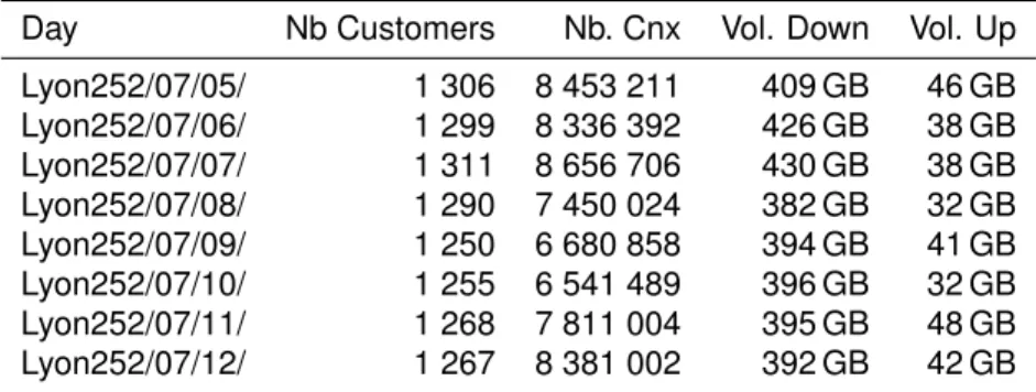
In Tab. 3.8, we sum up the total volumes (down and up), number of users and of con-nections for each day of capture. The average downstream rate per customer are quite low: around 5 kb/s if we consider 400 GB shared among 1000 users for 8 days. This mean that we shall focus on users generating most of the bytes (heavy hitters), or busy periods, in order to draw the characteristics of the platform.
3.2.6.2 Useful Connections
We define a useful connection as a connection with at least 1 kByte of downstream volume, and give in Tab.3.9the same figures as in Tab.3.8but considering only useful connections. The difference between Tab. 3.8 and 3.9 is mainly seen in number of connections and in upstream volume. The number of connections is approximately
Table 3.8: Distribution of Volume per Day (for Lyon probe)
Day Nb Customers Nb. Cnx Vol. Down Vol. Up
Lyon252/07/05/ 1 306 8 453 211 409 GB 46 GB Lyon252/07/06/ 1 299 8 336 392 426 GB 38 GB Lyon252/07/07/ 1 311 8 656 706 430 GB 38 GB Lyon252/07/08/ 1 290 7 450 024 382 GB 32 GB Lyon252/07/09/ 1 250 6 680 858 394 GB 41 GB Lyon252/07/10/ 1 255 6 541 489 396 GB 32 GB Lyon252/07/11/ 1 268 7 811 004 395 GB 48 GB Lyon252/07/12/ 1 267 8 381 002 392 GB 42 GB
Note the 10thJuly was a Sunday.
Table 3.9: Distribution of Volume per Day (for Lyon probe) only Connections larger than 1 kB in
downstream
Day Nb Customers Nb. Cnx Vol. Down Vol. Up
Lyon252/07/05/ 1 184 2 677 139 408 GB 39 GB Lyon252/07/06/ 1 182 2 831 656 425 GB 31 GB Lyon252/07/07/ 1 197 2 680 339 429 GB 32 GB Lyon252/07/08/ 1 154 2 553 930 381 GB 26 GB Lyon252/07/09/ 1 056 1 955 062 393 GB 36 GB Lyon252/07/10/ 1 033 2 132 712 395 GB 27 GB Lyon252/07/11/ 1 154 2 586 691 394 GB 38 GB Lyon252/07/12/ 1 143 2 617 861 390 GB 33 GB Inter Session Think TIME Session Session No flow for > 300s time < 300s
Flow Flow Flow Flow Flow Flow
Figure 3.8: Schema of session construction
divided by 4, whereas the upstream volume is decreased by about 20%. Downstream volume is almost unchanged. This is mainly due to P2P applications that generate a lot of very small connections.
3.2.7 Users’ Sessions
To figure out how the users behave we construct sessions as aggregation of connec-tions. We explain how we have constructed the sessions in Fig.3.8. This construction intends to mimic a usual activity pattern with multiple flows following each other with periods of silence (user’s think time) in between. We have chosen a threshold for inter-session of 5 minutes. We expect these inter-sessions correctly aggregate Streaming flows resulting from a continuous watch of multiple videos.
In Fig.3.9, we plot the CDF of session durations for all users. We also plot per user the median duration of its sessions. Note we consider only connections lasting more than 1 second for the session construction. The median session duration is at about
100 101 102 103 104 105 Session Duration in Seconds
0.0 0.2 0.4 0.6 0.8 1.0 P (X ≤ x)
Session Duration for Lyon all sessions: 19541
median session time per user: 1307 median session time per user (sessions longer than 300 sec): 1194 sessions longer than 300 sec: 7033
Figure 3.9: CDF of session durations for Lyon probe on 05/07 (only cnx > 1 sec)
100 101 102 103 104 105
Session Duration in Seconds
0.0 0.2 0.4 0.6 0.8 1.0 P (X ≤ x)
Session Duration for Lyon all sessions: 836
median session time per user: 177 median session time per user (sessions longer than 300 sec): 105 sessions longer than 300 sec: 298
(a) P2P flows only
100 101 102 103 104 105
Session Duration in Seconds
0.0 0.2 0.4 0.6 0.8 1.0 P (X ≤ x)
Session Duration for Lyon all sessions: 7137
median session time per user: 1058 median session time per user (sessions longer than 300 sec): 891 sessions longer than 300 sec: 3464
(b) Streaming flows only
Figure 3.10: CDF of session durations for P2P and Streaming for Lyon probe on 05/07 (only
cnx > 1 sec)
2 minutes globally: this seems quite low for a real user session. Thus, we also plot in this figure the same CDFs but with only sessions longer than 5 minutes. For these longer connections, the median is of about 15 minutes (1000 seconds) which seems more reasonable for a user’s session.
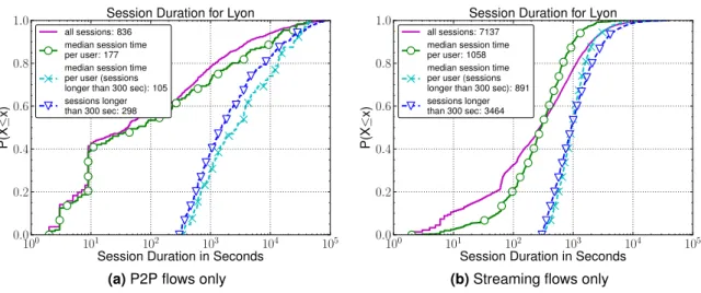
3.2.7.1 Sessions discriminated per Application
We have also conducted a session study based on the application used in Fig. 3.10. We focus on P2P and Streaming as their usage is quite different: background traffic for P2P vs. interactive usage for Streaming. Indeed we have much more short sessions for P2P than Streaming: 80% of Streaming sessions last more than 100 seconds whereas it’s only 50% of P2P ones. Focusing on sessions larger than 5 minutes, the distribution is similar between the two application classes.
100 101 102 103 104 105 Session Duration in Seconds
0.0 0.2 0.4 0.6 0.8 1.0 P (X ≤ x)
Session Duration for Lyon all sessions: 712
median session time per user: 522 median session time per user (sessions longer than 300 sec): 179 sessions longer than 300 sec: 197
(a) 4 am
100 101 102 103 104
Session Duration in Seconds 0.0 0.2 0.4 0.6 0.8 1.0 P (X ≤ x)
Session Duration for Lyon all sessions: 1256
median session time per user: 860 median session time per user (sessions longer than 300 sec): 577 sessions longer than 300 sec: 665
(b) 9 am
Figure 3.11: CDF of session durations per hour for Lyon probe on 05/07 (only cnx > 1 sec)
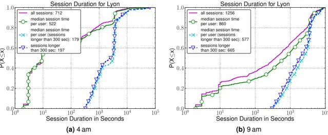
3.2.7.2 Sessions per hour
We study the impact of the time of the day on the session durations: as the application used change the session pattern, the time shall also have an impact. Indeed the appli-cation mix is different depending on the hour. We focus on two specific hours: 4 am and 9 pm in Fig.3.11aand 3.11brespectively. We have a very different pattern depending on the hour:
• at 4 am, most of the connections are shorter than 10 seconds; • whereas at 9 pm, most of connections are longer than 2 minutes.
This is obviously caused by the underlying applications, but the residential usage of the Internet is the root cause: mostly interactive usage in the evening vs. batch usage in the middle of the night.
3.2.8 User’s Level Analysis
In this section, we study the usage of applications by the customers. We first look at global trends for all the platform users, and then focus on the 4 customers generating most bytes in the platform.
3.2.8.1 Parallel Connections and Aggregated Throughput
In Fig.3.12a, we compute the CDF of the average downstream throughput per connec-tion (only connecconnec-tions larger than 1 MBytes). In this graph, we treat each applicaconnec-tion independently. A global remark is that very few connections achieve average through-put close to access rate: this means that the access rate to the Internet is not at all a bottleneck for connection throughput. The main point in this graph is that P2P con-nections achieve a very low average throughput: 90% of P2P concon-nections (larger than