Plane Strain Test for Metal Sheet Characterization
Paulo Flores1, Felix Bonnet2 and Anne-Marie Habraken3
1DIM, University of Concepción, Edmundo Larenas 270, Concepción, Chile 2ENS - Cachan, Avenue du Président Wilson 62, 94235 Cachan Cedex, France
3Department of ArGEnCO, University of Liège, Chemin des Chevreuils 1, B-4000 Liège, Belgium
Abstract
This article shows the influence of a plane strain test specimen geometry on the measurable strain field and the influence of free edge effects over the stress computation. The experimental strain field distribution is measured over the whole deformable zone of a plane strain test specimen by an optical strain gauge. The chosen material is the DC06 IF steel of 0.8 mm thickness. The stress field is computed for several geometries at different strain levels by a Finite Element (FE) commercial code (Samcef ®). The results show that the stress field is sensitive to the specimen's geometry and also to the tested material (strain field behavior is independent of material) and, based on results, an optimal specimen geometry is proposed in order to minimized the stress computation error.
Keywords: Material characterization, mechanical tests, stress - strain field homogeneity.
Introduction
Industrial requirements for lighter components and structures have motivated the study of material behavior in order to save manufacturing and transportation energy.
Different metal forming processes such as deep drawing, bending or stamping are required to manufacture automotive parts or beverage cans. The finite element method (FEM) is quite successful to simulate those metal forming processes, but accuracy depends both on the constitutive laws used and their material parameters identification.
Constitutive models for sheet metal forming at room temperature include a yield surface defined by a yield criterion, a normality rule and a hardening law (yield surface evolution). Accurate phenomenological yield criteria are defined by material parameters that must be identified by several mechanical tests such as uni-axial tensile test, equi-bi-axial test, bi-axial test, plane strain test and simple shear test.
The goal of this work is to define a plane strain test specimen geometry in which the stress and the strain tensor fields have a quasi-homogeneous behavior. A homogeneous behavior of those tensor fields allows the
computation of the stress state directly from the force and deformation data and simplifies the parameters identification routines.
The stress - strain state of the plane strain test and the experimental set up is described in next section. A strategy using FEM to study the stress field homogeneity is proposed in section 2. The results are discussed in section 3 and finally some conclusions are established and some perspectives proposed.
Regarding notation, lowercase bold-face Latin letters are used for vectors and uppercase boldface letters (Latin or Greek) to define second order tensor. The tensor product is defined by
Description of the Plane Strain Test
The plane strain test reproduces a particular case of the plane stress state in which one of the principal strain values and the shear components equal zero. This test is widely used in material characterization (yield surface and work hardening) and to obtain forming limits diagrams.
Mechanical Conditions
Fig. 1 sketches the axis over a laminated sheet. The material axes defined by the rolling direction (RD), the transversal direction (TD) and the normal direction (ND) are coincident with the X1, X2 and X3 axes. Assuming a
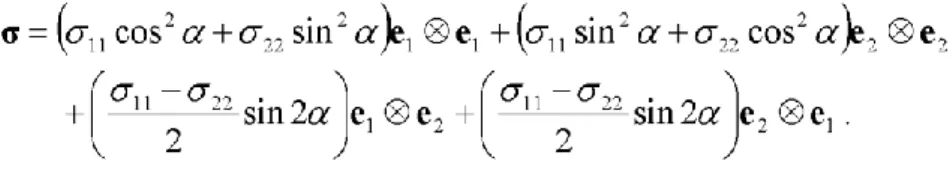
plane stress state, the second order Cauchy stress tensor can be defined as follows:
Figure 1: Rolled sheet axis definition, α defines the angle with respect to the RD.
To represent the stress state for any angle a the following transformation linking a state defined in the x1, x2 and
x3 axes with the X1, X2 and X3 is used:
where R is a proper orthogonal second order tensor (i.e. RTR = RRT = I and det R = 1) defined by
Then, the general expression for the plane stress state is defined as follows:
The principal stretches of the sheet are represented by λi (i = 1, 2, 3) in the second order stretch tensor U:
The logarithmic strain is defined in terms of the principal stretches as:
For the plane strain case λ2 = 1, then ε2 = 0. Assuming volume conservation, i.e., λ1λ2λ3 = 1 (or ε1 + ε2 + ε3 = 0),
In plasticity, the plastic strain rate tensor is related to the Cauchy stress tensor by the normality rule:
where is the plastic multiplier and is the plastic potential function represented, in this work, by the Hill 1948 orthotropic yield criterion [1]:
H, G, F, N, M, L are material parameters and k(p) describes the yield surface size evolution (isotropic hardening) in terms of the equivalent plastic strain.
Using the condition ε2 = 0 one can assume that:
which allows the representation of one component of the Cauchy stress tensor in terms of the other (Eq. 10). This has particular significance when the stress data is used to identify yield function material parameters (e.g. when using the "plastic contours method" [2,3]) since most of the testing machines do not count with a proper device to measure the stress component in perpendicular direction with respect to the applied load. Eq. 10 can be seen as a generalization of the isotropic case when ka = 0,5. The relation shown in Eq. 10 can be obtained for
other yield criteria as it is shown in [4].
Experimental set up
Fig. 2a shows the bi-axial testing machine built at the ArGEnCO Laboratory at the University of Liege [5]. The arrows in the figure show the machine movement axes. The motion is generated by two hydraulic pistons, which can be controlled in displacement or force simultaneously or independently. These motions enable us to perform simple shear and plane strain tests. Fig. 2b shows a detail of the specimen's measurable zone clamped by hydraulics grips.
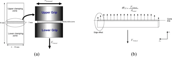
The specimen geometry designed for the bi-axial testing machine is shown in Fig. 3a where the dotted area is the measurable zone. The deformation is imposed by the pistons (vertical for the plane strain test and horizontal for the simple shear test) of the bi-axial testing machine. The strain field can be measured in the whole deformation zone (due to an optical strain gauge), and the average stress σ11 is computed form the load cell data and the actual
area as it is shown in Fig. 3b. This assumption is only valid if the stress field is homogeneous. The component σ22 of the stress tensor cannot be measured with this mechanical configuration.
Figure 2: Bi-axial testing machine designed at the ArGEnCO Laboratory, University of Liege.
Figure 3: (a) Specimen geometry and deformation area, (b) Sketch of the stress distribution.
Fig. 4 shows the experimental strain field distribution at the centerline level (Fig. 3b) for the logarithmic strain tensor components ε11 and ε22. The test is done over a DC06 IF steel of 0.8mm thickness (anyways, the strain
distribution is independent of the material). The following conclusions can be drawn from these results: the strain tensor is homogeneous over the deformation area except at the free edges, the homogeneity depends on the amount of the imposed deformation (ε11), the strain component ε22 is negligible in the homogeneous zone of the
deformation area and, by volume conservation, the condition ε1 = -ε3 is valid over the homogeneous zone of
the deformation area.
These conclusions are valid for the specimen geometry of Fig. 4a, i.e., when h/b=10.
The influence of deformation area geometry, the imposed strain level and the material over the stress field is studied in what follows by a FE simulation of the plane strain test.
Figure 4: (a) ε11 strain distribution over the specimen centerline, (b) ε22 strain distribution over the specimen centerline.
Plane Strain Test FE Simulation
The FE simulation of the test is used to study the stress field distribution over the deformable zone of the specimen. By studying the influence of the edge effect over several geometries, the obtained results help to define a criterion to define whether a stress field can be consider (quasi)-homogeneous or heterogeneous. Simulation Parameters
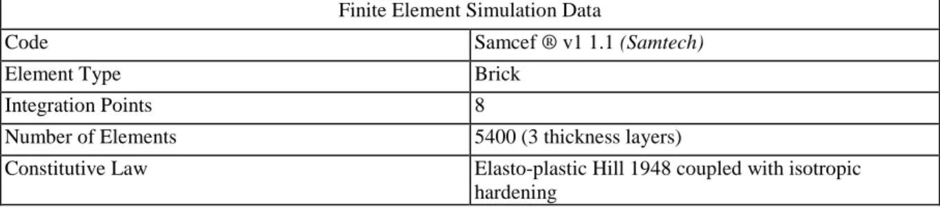
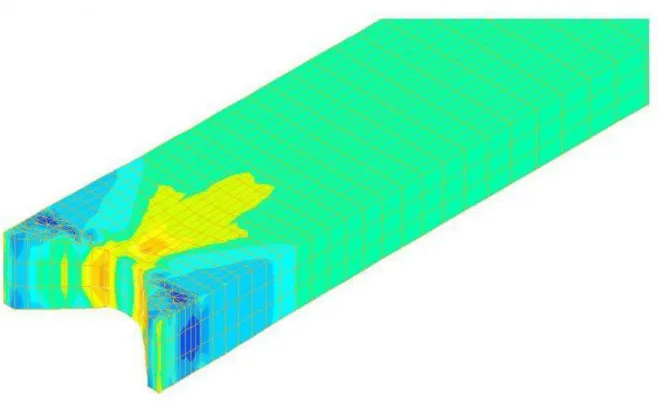
The simulation parameters appear in Table 1 and only the deformation area is simulated (sliding of the specimen inside the grips is neglected), the used mesh appears in Fig. 5. To study the influence of the material in the stress field, the results obtained out of two materials are compared. Material 1 corresponds to the IF steel DC06 characterized in [3,5], Material 2 is a Active material that has the same initial yield locus as Material 1, but a different hardening behavior (hardening stagnates at 10% of deformation). The initial yield locus material parameters for the Hill 1948 criterion (Eq. 8) are in Table 2 and Table 3 contains the hardening parameters. The elastic modulus is E = 210000 [MPa] and Poisson's coefficient v=0.3.
Table 1: Finite element strategy.
Finite Element Simulation Data
Code Samcef ® v1 1.1 (Samtech)
Element Type Brick
Integration Points 8
Number of Elements 5400 (3 thickness layers)
Constitutive Law Elasto-plastic Hill 1948 coupled with isotropic hardening
Table 2: Initial yield surface material parameters for Hill 1948 criterion.
Material Parameters for Hill 1948 criterion
H F G N M L
[MPa] DC06
0.8mm
1.13 0.69 0.87 3.26 3.26 3.26 140.47
Table 3: Hardening laws material parameters.
Material Parameters for Hardening Laws
Hardening Law Material Parameters
Material 1
(DC06 0.8mm) k(p)=K(ε0+p)n
K [MPa] ε0 n
517.4 0.007 0.26
Material 2 k(p) = σy+ RSAT [1-exp(-CRp)] σy [MPa] RSAT [MPa] CR
140.47 370 30
Comparing Variables
The average stress is defined by Eq. 11, here Vi represents the volume of the element, Vtotal the total volume of
the deformable area and σi is the stress value of the element (in the loading direction). This stress computation is
impossible to obtain experimentally.
A second stress definition is given by Eq. 12. F is the load measured by the load cell and ACL is the cross section
experimentally but it involves expensive equipment and it is time consuming. A third definition is presented in Eq. 13. F is the load measured by the load cell and ACP is the cross section area computed with the information
obtained at the center point of the specimen's deformation area. Assuming volume conservation in plasticity, this cross section area can be obtained from Eq. 14, where A0 is the initial cross section area of the specimen and
εCP
11 is the strain measured in the load direction at the center point of the deformation area.
Then, in order to define a homogeneity criterion, the stress values obtained from Eq. 12 and 13 are compared with the one given for Eq. 11 for a quasi-homogeneous, arbitrary chosen, stress distribution. This reference stress is obtained from a geometrical ratio of h/b=20 (a higher ratio would not be economically viable) and t=1.5mm since the absolute relative error between σglobal (or σtrue) and σave is not greater than 0.5% for an imposed strain of 20% for Material 1 (see Fig. 5) and 10% for Material 2.
Results
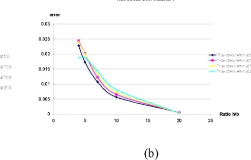
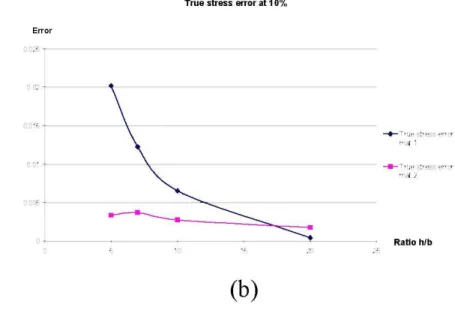
Fig. 6 shows the error at different strain levels for different specimen's geometries. It is clear that increasing the ratio h/b, the error between the average stress (taken as a reference value) and the global and true stress diminish. The influence of the strain level does not seem to have a large influence on the error evolution.
The error obtained by using the true stress definition is less than 0.2% in the most adverse case (h/b=5) when comparing with the error given by the global stress definition, this means that for a ratio higher than h/b=10 the actual area can be obtained from measures taken at the center of the specimen (Eq. 14), saving important data processing time.
Fig. 7 shows that the stress error depends on the material (unlike the strain fields), hence it makes impossible to compute a general correction factor.
Conclusions and Perspectives
The geometrical ratio h/b=10 in the measurable zone of the specimen geometry seems to be the most performing since the stress error is less than 1% for the two materials. It also ensures that the strain in the sense
perpendicular to the impose deformation ε22 remains negligible during the deformation process. The actual area
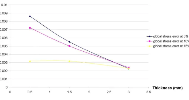
can be measured from the center point data. The thickness variation does not seem to contribute significantly to the stress error.
Even if the final stress error could be quantified, this has not practical interest since the stress field is dependent on the material; hence it is impossible to define a general correction factor.
From this work another criterion of homogeneity can be proposed in order to neglect the component ε22 in the
strain tensor: the strain average taken over an 80% of central part of the deformation area must by much lower than the one measure at the free edges (as observed in Fig. 4b). In this case, it is necessary to compute the whole strain field.
In future, the specimen geometry will be slightly modified at the free edge level (Fig. 9) in order to study the failure position which occurs near the free edges, where strain and stress concentrations are higher as it is shown respectively in Fig. 4 and Fig. 5.
Acknowledgement
As Research Director, Anne-Marie Habraken would like to thank the National Found for Scientific Research (FNRS, Belgium) for its support.
References
[1] R. Hill: The Mathematical Theory of Plasticity (The Oxford Eng Sciences Series, 1950). [2] T. Kuwabara, A. Van Beal, E. Iizuka: Acta Materialia Vol. 50 (2002), pp. 3717 - 3729.
[3] P. Flores, P. Moureaux, A.-M. Habraken: Material Identification using a Bi-axial Test Machine (Trans Tech Publications, Switzerland 2005).
[4] P. Flores: Development of Experimental Equipment and Identification Procedures for Sheet Metal Constitutive Laws (PhD Thesis, University of Liege - Belgium, 2005).
[5] P. Flores, E. Rondia, A.-M. Habraken: International Journal of Forming Processes, Special Issue (2005) pp. 117-137.