HAL Id: hal-01856844
https://hal.archives-ouvertes.fr/hal-01856844
Submitted on 17 Aug 2018HAL is a multi-disciplinary open access archive for the deposit and dissemination of sci-entific research documents, whether they are pub-lished or not. The documents may come from teaching and research institutions in France or abroad, or from public or private research centers.
L’archive ouverte pluridisciplinaire HAL, est destinée au dépôt et à la diffusion de documents scientifiques de niveau recherche, publiés ou non, émanant des établissements d’enseignement et de recherche français ou étrangers, des laboratoires publics ou privés.
Dimensional analysis and surrogate models for the
thermal modeling of Multiphysics systems
Florian Sanchez, Marc Budinger, Ion Hazyuk
To cite this version:
Florian Sanchez, Marc Budinger, Ion Hazyuk. Dimensional analysis and surrogate models for the thermal modeling of Multiphysics systems. Applied Thermal Engineering, Elsevier, 2017, 110 (3), pp.758-771. �10.1016/j.applthermaleng.2016.08.117�. �hal-01856844�
1
Dimensional analysis and surrogate models for the thermal
modeling of Multiphysics systems
Florian Sanchez
Institut Clément Ader, UMR CNRS 5312, Université Paul Sabatier (UPS) 3 rue Caroline Aigle, 31400 Toulouse
[email protected] Marc Budinger*
Institut Clément Ader, UMR CNRS 5312, INSA Toulouse 3 rue Caroline Aigle, 31400 Toulouse
[email protected] Ion Hazyuk
Institut Clément Ader, UMR CNRS 5312, INSA Toulouse 3 rue Caroline Aigle, 31400 Toulouse
[email protected] ABSTRACT
This paper presents an original form of surrogate models and the associated construction procedure adapted to the thermal modeling of Multiphysics systems. This method of meta-modeling, which uses dimensional analysis, extracts compact models suitable for preliminary design from finite element simulations. The mathematical expression used for the model is a product of variable power laws of dimensionless numbers. Compared to traditional surrogate models (polynomial response surfaces, kriging and radial basis functions), it has the advantage of giving light, compact forms with good predictive accuracy over a wide range of the design variables (several orders of magnitude). The general regression process is first explained and illustrated with a study of the Marangoni effect. Then the methodology is used to build thermal models of an electromechanical actuator (EMA) which are used to size an aileron EMA for two different cooling strategies. Finally the models are also used to discuss the effect of confinement on the actuator’s overall thermal resistance.
Keywords
Thermal modeling, Response Surface Methodology, Surrogate modeling, Dimensional analysis, Convection cooling, Aerospace actuators.
INTRODUCTION
A technology shift towards more electric solutions is emerging in aerospace systems [1]. New technology brings new challenges, especially for the preliminary design process of these systems, which are becoming more complex with new functions, new domains, and new components. Unlike in hydraulic power systems, where the heat losses are evacuated by the working fluid, in the more electric systems the heat generated needs to be dissipated by the system’s own components.
2
Thus, the exploration of the design space and the optimization of these Multiphysics systems involve modeling the heat exchanges between the different components. This article focuses on thermal models suitable for use at system design level, where the thermal behavior of the components has to be estimated with a limited number of input variables, which may vary over wide ranges. Therefore, it is crucial for the models used at this design stage to be: simple – for rapidity and easy handling, i.e. simple algebraic or ordinary differential equations that can be easily implemented in worksheets, system level modeling [2] or optimization loops; explicit – to enable analytic manipulations that provide direct access to the main integration parameters (mainly weight and geometrical parameters) while having very little input information available (usually functional requirements); continuous – at least in the range of parameter variation conventional for the given application, which is especially useful for the optimization; broad in validity range – models have to be usable and reusable over large ranges of validity of variables to allow the capitalization of knowledge and optimization without a priori.
The approaches used to generate such models may take different forms. A classical way of working is to solve physical equations analytically after simplification of the geometry or by neglecting some physical phenomena. The literature offers a large number of correlation laws in heat transfer for simple geometries [3]. The validation of these analytical models is usually carried out on more detailed models (finite element models – FEM) or on experimental or statistical data [4]. This approach requires expertise and becomes difficult for Multiphysics systems. A second approach uses empirical models [5]. These are mainly regression models based on physical experiments and may become expensive if a large number of experiments are required. Additionally, it may be difficult to vary all the main sizing parameters. Yet another approach uses response surface methodology, surrogate models or meta-models of computer experiments. This is widely used in thermal engineering applications such as optimization of the thermal placement of multichip modules [6], optimization of heat exchangers or heat sinks [7–9] or specific analysis in heat pipes [10]. The next section of this article assesses the state of the art of the mathematical forms of models associated with these approaches.
The purpose of this paper is to provide a method to construct surrogate models adapted to heat transfer problems and suitable for the wide range of variation of input variables often encountered in preliminary design of Multiphysics systems. This is achieved via an extension of the metamodeling approach in combination with the use of dimensional analysis [11,12], the Buckingham theorem [13]. The main contributions of the paper are the general mathematical form of the model proposed and the method that enables its final expression to be narrowed down. Section 2 presents the proposed methodology and the different steps for the construction of a surrogate model. Section 3 illustrates the process with the thermal modeling of an electromechanical actuator (EMA) used to control the aileron of an aircraft. Section 4 presents different possible uses of the thermal models built using the proposed methodology.
1. State of the art on mathematical forms of approximations
This state of the art deals with approximation techniques employed in computer experiments and using parametric regressions. It focuses especially on the mathematical forms of these approximations. The design of experiments (DOE) and
3
model building methods will not be discussed here. For more details on these aspects the references [14–18] can be consulted.
The subject here is to identify and compare the different possible forms of approximation functions f:
= ( , , … , , , … ) (1)
where:
• is the physical characteristic of a component that is useful for its selection in a system, such as the heat transfer coefficient of a heat exchanger, the thermal resistance of a component, etc.
• are the geometrical dimensions of the component, these dimensions may vary over large intervals during global system design.
• are boundary conditions or material properties used in the design of the components.
It is important to note that and are independent variables and is a dependent variable.
1.1.Pure mathematical approaches
Response surface models, meta-models or surrogate models are relatively simple mathematical relationships between input variables, physical parameters and output response:
= ( , ) (2)
where:
• is a vector of physical parameters , = 1, … , , considered to be input variables and which can be design variables such as dimensions , boundary conditions or material properties ;
• is a vector of parameters associated with the family of functions needed to construct the surface.
Parametric regressions are based on models requiring the estimation of a finite number of parameters, θ, that express the effects of basis functions on the response surface. With polynomial interpolation or regression [15] described by equation (3) in Table 1, the basis functions are 1, , , … , . The idea is to obtain a surface that is differentiable and continuous. Higher orders of Taylor expansion will usually yield a more accurate approximation. However, the greater the number of terms is, the more flexible the model becomes, but the response may be corrupted by over-oscillations.
Other meta-model families assume that samples taken close to each other are likely to have highly correlated response values, whereas samples taken far apart are not. Radial basis functions, which are radially-symmetric functions, and Kriging methods [19,20] are thus underpinned by the idea that the sample response values exhibit spatial correlation. RBF and Kriging methods have been found useful for modeling general surfaces that have many peaks and valleys and when exact interpolation of samples is desired. A common choice for the basis functions of RBF are the Gaussian functions as illustrated in Table 1 with equations (4) and (5), where represents the mean value of the experiments.
4
Generally for all these forms of regression, errors become very large outside the range they were built (extrapolation). RBF and Kriging methods are well suited to the representation of complex behaviors on well-defined and relatively small ranges of the inputs. They are therefore particularly used in component design and optimization but are less suitable to representing the characteristics of components during a global system design.
Table 1: Synthesis of mathematical forms of pure mathematical approaches
Approaches Mathematical form of the model Equation
references Literature references Response surface methodology (RSM) = ( , ) = + + (3) [15] Radial basis functions (RBF) = ( , ) = + !" !(#)" $ %$ = + & !'()!() (#)'$ %$ *+ (4) [19]
Kriging functions = ( , ) = + & !
'()!() (#)',)
%)$
*+
(5) [20]
1.2.Approaches based on dimensional analysis
There is an alternative school that suggests building models by relying more on physical reasoning than on mathematical approaches. Dimensional analysis is a powerful way to do this and is mainly based on the Buckingham theorem [11,13]. According to this theorem, Equation (1) can be rewritten in the form:
= - . , , … ,011121113/ /
4 (6)
where:
• are dimensionless variables, also called dimensionless numbers
• 5 is the number of dimensionless numbers, which depends on the 6 independent physical units (e.g. m, kg, s, etc.) and the variables involved in the problem. It is calculated using the relation: 5 = − 6.
The output response, y, is also modified to become dimensionless: = & 8# 9#
(7)
This approach, classical in fluid mechanics and heat transfer [3], often uses products of power laws with dimensionless numbers , Equation (8) in Table 2, to represent the function -. The coefficients : in Equation (8) can be obtained by first order linear regression on a logarithmic scale. The SLAW method has the same type of mathematical expression but, instead of dimensionless numbers, it uses the physical variables directly [21] (Equation (9) in Table 2). Homogeneity in terms of dimensions is ensured by imposing constraints on power coefficients. Assuming that all the
5
dimensionless numbers , ∈ 1, … , 5 of the function - are constants implies that is constant as well. Thus the dependent variable can be expressed in the form of a scaling law, Equation (10) in Table 2, where < is the characteristic length of the system. This mathematical form enables the main behavior of mechanical [22] or mechatronic components [23] to be represented in a simple way. The SLAWMM method [24,25] extends the validity of scaling laws by replacing the = and : constant coefficients in equation (10) by functions of numbers (Equation (11) in Table 2). The regressions obtained have been compared to classical meta-models and show the interest of the physical basis of scaling-law-based meta-models for preliminary sizing of components: their shape is easy to handle while remaining valid over a wide range of sizes, for prediction or even extrapolation purposes. Other authors [26–28] have represented - by a polynomial function with , (Equation (12) in Table 2) and have been able to show robustness of regression: reduction in the number of variables manipulated, decrease in the size of the DOE (decreased workload) and increase in the accuracy. Some authors [29,30] have proposed a combination of polynomial and power law meta-models with and their associated procedure for model building. This form of model represents a generalization of power law expression. The drawback of this method is that it requires non-linear regression.
Table 2: Synthesis of mathematical form of DA based approaches
Approaches Mathematical form of the model Equation references Literature references
Power laws with
numbers = : &
8#
/
(8) [3]
SLAW method: Power laws with
numbers
= : & 8#
(9) [21] Scaling laws = =<8
(10) [22,23]
Scaling law meta-models (SLAWMM) = (<, , , … ) = =( , , … )<8(>?,>$,… ) with =@A# (11) [24,25] Polynomial meta-models with numbers = : + : / + :B B 5 B= 5 =1 (12) [26–28]
Sum of power law
meta-model = β D
E
& F#)
/
(13) [29,30]
2. VPLM: Variable Power Law Meta-model
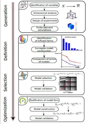
The methodology presented here is called the Variable Power Law Meta-model (VPLM). It is applied in four main steps: data generation, surrogate model definition, surrogate model selection and validation, and surrogate model
6
optimization. Figure 1 shows the global process of the methodology by presenting all the processes involved in each main part.
Figure 1: Procedure of the VPLM methodology
This methodology aims at facilitating the thermal modeling and, at the same time, the design of Multiphysics systems by building surrogate models based on dimensional analysis and finite elements simulations.
2.1.Data generation
This step is composed of four operations. The first one deals with the identification of the influent variables. Sensitivity analysis or screening methods [31,32] can be used here. Then dimensional analysis is performed on the physical variables to build the corresponding dimensionless numbers. More details on dimensional analysis can be found in [11,12]. The number of dimensionless numbers is determined using the modified form of the Buckingham theorem proposed by Sonin [33]. This theorem suggests separating constant physical parameters from variable ones. In some cases, this consideration enables the set of dimensionless numbers to be reduced. Afterwards, a design of experiments is established to define the configurations that have to be simulated in finite element simulation software. As will be shown in the following section, the VPLM methodology, which is based on linear regression, can work with different types of design of experiments (Full Factorial design, Latin Hyper Cube design, etc.).
7
2.2.Surrogate model definition
This second step deals with the definition of the surrogate model or, in other words, the algebraic expression of the model. As the name of the methodology (VPLM) indicates, the mathematical form of the chosen function is a variable power law. This choice was motivated by a variety of observations and studies of the state of art concerning the approximation models used in engineering. Although polynomial models are often used to build response surface models, many engineering problems follow a power law behavior [34,35]. In addition, for heat transfer problems, the correlations most commonly used to estimate the heat transfer coefficient are power law functions [3,36,37]. Regarding these observations, the most appropriate surrogate model form may be:
π = =π8?π8$… π
/ 8H
(14)
where is the dimensionless number containing the output, = and : are numerical coefficients, and are dimensionless numbers.
The relation (14) re-written in logarithmic scale corresponds to a response surface model of the first order (15).
log( ) = log(=) + : log ( ) /
(15)
However, the literature on correlation laws used in heat transfer shows that power law functions of dimensionless numbers do not represent all the configurations generally encountered [38]. Very often, the authors provide charts or tables with numerical values to be used for = and : depending on the value of dimensionless numbers. Thus, since engineers advise increasing the order of the polynomial model when its accuracy is not sufficient [39], we propose to increase the order of the model in Equation (15). In order to keep the algebraic model simple, the VPLM methodology will estimate at most third-order models. Thus, the general form of the proposed model is:
log( ) = log(=) + : log ( ) /
+ L log( ) logM N
/ /
+ O *log( ) logM N log( *)
/ * /
/ (16)
where =, : , L and O * are numerical coefficients. By rewriting relation (16) in the linear scale, we obtain a variable power law model:
π = =π8?(>?,>$,…,>H)π8$(>?,>$,…,>H)… π8HM>?,>$,…,>HN
(17)
8
Most of the time, the model does not need to keep all the higher order terms1 in Equation (16). In order to identify which ones deserve to be kept, a sensitivity analysis [40] is conducted using the simulation data coming from the first step. Then, they are sorted in order of their importance (Figure 2) and 6 models are automatically calculated where, for the PQ model, ∈ 0,1, … 6 − 1 , only the first higher order terms from Figure 2 are considered. Note that for = 0 the model obtained is identical to the one in Equation (14). The models are built by minimizing the least square error between the model and the simulation data [39].
2.3.Surrogate model selection and validation
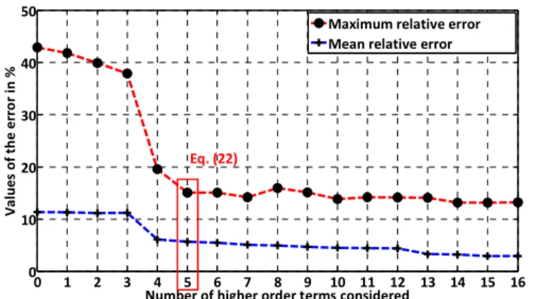
This third step of the VPLM methodology concerns the selection of the appropriate model and its validation regarding its accuracy and complexity. During the previous step, several candidate models were built and now we can evaluate the relative errors and/or the standard deviation for each one. In order to appreciate the accuracy of each model, it is possible to use scatter plots (simulation data versus the data calculated with the model) as in Figure 3. However, if all the different VPLM models are to be compared, scatter plots may be inconvenient. A more convenient way to compare the surrogate models built during the second step is to represent the evolution of the relative errors of each model (differing in the number of higher order terms selected), as shown in Figure 4. As the evolution of VPLM models follows the horizontal axis, which corresponds to the arrangement of the terms from Figure 2, it can be seen that the prediction accuracy increases with the number of terms selected, but the model also becomes more bulky. Thus the engineer can choose a compromise between accuracy and the simplicity of the expected surrogate model.
Figure 2: Example of arrangement of higher order terms according to their importance for the case of two
dimensionless numbers (ST= UVW(XT))
Figure 3: Example of scatter plot (''X=Y'' diagram) to appreciate the accuracy of a model
1 Here, the higher order terms are those multiplied by L and O
* 0 0.1 0.2 0.3 0.4 0.5 0.6 C o e ff ic ie n ts v a lu e s Π1.Π 2 Π1.Π 1 Π2.Π 2 .Π1 Π2.Π 2 Π.2Π 2 .Π2 Π1.Π 2 .Π1 Π1.Π 1 .Π1 10-2 10-2
Π0 calulated using the simulation (reference) Π0 e st im a te d ( m e ta -m o d e l) VPLM Max error : 15.0 % Mean error : 5.1 % y=x
9
Figure 4: Example of comparison of relative errors between different models
2.4.Optimization of surrogate model form
Even though many models involved in heat transfer problems follow a power law behavior, in some cases this mathematical form may not give the expected accuracy. This step of the VPLM methodology gives the possibility of optimizing the surrogate model form in order to achieve the expected accuracy. In this way, this last step of the methodology allows us to change the mathematical form for one or more dimensionless numbers involved in the meta-model. Figure 1 shows the three sub-steps of this form optimization step.
There is no restriction on the new form selected; all the mathematical forms presented in the state of the art may be used (Table 1 & Table 2). For example it is possible to move from a classical power law with two dimensionless numbers to a combination of power law and polynomial function.
Since the new form chosen is nonlinear, nonlinear regression in the least squares sense is used to determine the numerical values of the coefficients involved in the model. A scatter plot as “X=Y” diagram may be used to compare the precision between the new model and the old one.
2.5.Marangoni effect: Evaluation of the heat transfer coefficient 2.5.1. Application of the VPLM methodology
Here we propose to study the heat transfer due to the Marangoni effect [41]. Marangoni convection occurs when the surface tension of an interface (generally liquid-air) depends on the concentration of a species or on the temperature distribution (thermo-capillary convection). The aim of this study is to use the VPLM methodology to build a model able to calculate the global heat transfer coefficient of a cavity subjected to a temperature gradient that induces a flow through the Marangoni effect. Figure 5 shows the configuration of the geometry and the boundary conditions used for the study.
10
Figure 5: Configuration of the study for the Marangoni effect (YZ[\= ]^^_)
The governing equations of the problem are the Navier-Stokes equations using the Boussinesq approximation, the Energy equation and the following equation, which describes the Marangoni effect on the liquid-air interface:
`a
` = b`c` (18)
where b [d/6/f] is the temperature derivative of the surface tension g.
The global heat transfer coefficient hjjj depends on eight physical variables (Equation (19)) and, according to the i Buckingham theorem, it may be written in dimensionless form as in Equation (20).
hO
jjj = (k,l,m , ,<i, ni, opΔc, bΔc) (19)
da = -MrsAt, us, v, wtN (20)
where v=xvyzAt
{$ represents the ratio between the thermo-capillarity forces and the viscous forces and wt =wAtt
represents the aspect ratio of the cavity. In addition, the number of dimensionless variables may be reduced by combining the Prandtl number, us, and v into a single dimensionless number. This new dimensionless number is the Marangoni number, which represents the ratio between the surface tension forces and the viscous forces.
da = -MrsAt, |o, wtN (21)
It is assumed that the properties of water are constant and are evaluated at the mean temperature. A latin hyper cube sample (LHS) containing 64 configurations is built to define all the configurations that have to be simulated according to the ranges defined in Table 3. The finite element simulations are performed in COMSOL Multiphysics and Figure 6 shows different results for different flow regimes.
11
}~•€ = •. ƒ ∙ …^…, †W = ‡. ˆƒ ∙ …^ƒ, X‰€ = …. … }~•€= …. ˆˆ ∙ …^Š, †W = ˆ. ‹] ∙ …^Œ, X‰€= ^. ƒ•
}~•€ = ‹. •‹ ∙ …^ƒ, †W = Ž. ‹• ∙ …^], X‰€= ^. •‹ }~•€= …. •ˆ ∙ …^ˆ, †W = …. ]Ž ∙ …^ˆ, X‰€ = ^. •ˆ
Figure 6: Results from FEM simulations for different flow regimes (Temperature field [°K] and streamlines) Table 3: Ranges for the design of experiments used for the study of the Marangoni effect
Variables Units Ranges
ni 66 5 − 10 <i 66 5 − 30 Δc f 0.1 − 1 rsAt - 5 ∙ 10 − 1 ∙ 10‘ |o - 6 ∙ 10 − 4 ∙ 10Š wt - 0.25 − 1.5
From the results of the finite element simulations, the VPLM methodology is used to generate different models, the relative errors of which are represented in Figure 7. The model with five higher order terms reaches 15% of maximum relative error and represents the best compromise between accuracy and complexity.
12
Figure 7: Evolution of the relative errors for the study of the Marangoni effect da•–A— = 1.7 ∙ 10!ŒrsAt
! . ™š› .Œ ‘ œ•žMŸ ¡tN œ•ž(—¢)! . Œ œ•žMŸ ¡tN œ•žMŸ ¡tN› . Œ™ œ•žM>£tNœ•žMŸ ¡tN
|o .™Š‘! . ŠŠ œ•žM>£tN œ•žMŸ ¡tN! . ™ œ•ž(—¢) œ•žMŸ ¡tN wt.Œ
(22)
2.5.2. Comparison with other surrogate modeling techniques
Here we propose to compare the VPLM methodology with other surrogate modeling techniques such as Radial Basis Function (RBF) and Response Surface Methodology (RSM). These two techniques are widely used to build models from finite element simulations [8,42]. The RBF and RSM models are built on the same design of experiments as the one used for the VPLM model and the comparison is made on another design of experiments to evaluate the prediction capability of the models. Equations (23) & (24) show the RBF model and the RSM model, respectively, built for the Marangoni study. The RSM model is a third-order polynomial model that uses the same number of numerical coefficients as the VPLM model.
da¤¥¦( ) = + p §Š exp «−‖ − ‖2g - (23) da¤®— = 0.95 + 1.56 ∙ 10−5rs<O+ 5.38 ∙ 10−5|o +2.64 ∙ 10!Šrs At wt− 0.255 wt wt− 2.64 ∙ 10!±rsAt|o +8.51 ∙ 10! ‘rs AtrsAt|o − 1.97 ∙ 10!ŠrsAt wt wt (24)
A LHS of 27 points is built according to the ranges described in Table 3 to define the configurations that have to be simulated. Figure 8 presents a scatter plot comparing the results of the finite element simulations with those predicted by the models. This comparison shows that the VPLM methodology offers models with a better prediction capability than the RBF and RSM techniques do. In addition, the VPLM model offers a lighter and explicit expression, which allows mathematical manipulations. 0 1 2 3 4 5 6 7 8 9 10 11 12 13 14 15 16 0 10 20 30 40 50 V a lu e s o f th e e rr o r in %
Number of higher order terms considered Maximum relative error Mean relative error
13
Figure 8: Comparison between different surrogate modeling techniques for the Marangoni effect study
3. Application to the thermal modeling of an electromechanical actuator
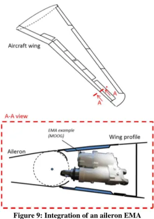
The VPLM methodology will be applied to the electromechanical actuator of an aileron. The main components used are generally an electric motor, a roller-screw and a housing containing all these components. Figure 9 shows the integration of this type of actuator into an aircraft wing. Generally actuator integrators/manufacturers start the design of actuators by considering only natural convection cooling and model it using correlation laws defined for infinite domains. Then, flight or ground test campaigns help to improve the thermal modeling of the actuator. As illustrated in Figure 9, the actuator is located in a confined space and, as shown by Atmane et al. [43] and Sebastian et al. [44], this confinement has a non-negligible influence on the natural convection phenomenon. For this reason, actuator manufacturers need representative correlation laws to be able to take a more realistic cooling configuration into account earlier in the design.
10
010
0Nusselt number evaluated by FEM
N u ss e lt n u m b e r p re d ic te d b y t h e m o d e ls Nu RBF Max error : 39.4 % Mean error : 11.8 % Nu RSM Max error : 78.2 % Mean error : 19.0 % Nu VPLM Max error : 22.9 % Mean error : 5.5 % y=x
14
Figure 9: Integration of an aileron EMA
This paper studies two different cooling strategies conceivable for an aileron EMA: natural convection cooling in a confined space (Figure 10) and forced convection cooling in a confined space (Figure 11). The two-dimensional approximation is justified by the fact that the actuator has to be cooled only by the surrounding air and conductive heat transfer toward the structure is usually prohibited by the airframers. Also it is assumed that the actuator is the same length as the rectangular cavity. The approach proposed here is to model the actuator (Multiphysics system) as an assembly of models of different components and to use the VPLM methodology to generate the thermal models. In this way, the modeling of the heat transfer of the EMA uses three different thermal models: (1 in Figure 10 and Figure 11) a conductive model of the brushless motor, and (2 and 3 in Figure 10 and Figure 11) a conducto-convective model of the housing in its environment for two different cooling configurations (natural and forced convection). Additionally to these heat transfer models, thermal loss models also have to be considered. The latter were developed in previous works, i.e. loss models for the roller screw (given in [23]), loss models for the motor (iron and copper losses given in [45]), and a surrogate model for the motor torque calculation obtained with the VPLM methodology in [46]. All the models together enable the main lengths of the actuator and its components to be linked to the hot spot temperature of the motor, which is the critical characteristic to be considered for actuator sizing.
15
Figure 10: Modeling of the EMA in its environment with natural convection cooling
Figure 11: Modeling of the EMA in its environment with forced convection cooling
3.1.Conductive model of the brushless electric motor
The VPLM model that will be built here is based on the two-dimensional finite element model of an electric motor, represented in Figure 12. It corresponds to a motor from the PARVEX NX range [47], the characteristics of which are in accordance with the specifications for aileron application. The objective is to construct a model able to calculate the conductive thermal resistance ²i@ between the motor hot spot, which is located at the center of a slot (cf. Figure 13) and its external surface (the one in contact with the housing). The thermal losses dissipated in each slot of the motor stator are mainly Joule losses. The temperature on the external surface of the motor c³´ µ is imposed to enable the calculation of the temperature difference Δ = cQ¶P− c³´ µ, cQ¶P being the temperature of the hot spot. Table 4 gives the material properties used for the finite element simulations.
Table 4: Material properties of the electrical brushless motor
Ref. in Figure
12
Material l ·¸/6/f¹
16 2 Copper & Resin [48] (lº´, l »³, ¼E, <E) ½ 0.7 3 Nomex ( ¾) ½ 0.1 5 SmCo (Magnet) 10 6 Air ~0.02
Figure 12: Finite element model of the electrical brushless motor
Figure 13: Finite element simulation results for the conductive model of the brushless electric motor (COMSOL Multiphysics)
The linear2 conductive thermal resistance of the electric motor <
E²i@ depends on five variables:
<E²i@ = (¼E, ¾, l ¶ , l¾, lE () (25)
where: ¼E is the diameter of the motor, ¾ the thickness of the Nomex insulation, l ¶ the thermal conductivity of the iron, l¾ the thermal conductivity of the Nomex, and lE ( the thermal conductivity of the copper-resin mixture. Applying the Buckingham theorem modified by Sonin [33] leads to the following dimensionless form of Equation (25):
i@ = -( ) (26)
where: i@ = l ¶ <E²i@ and =ÀÁ »Â.
A full factorial DOE of fifty points is built according to the ranges defined in Table 5. The defined configurations are simulated using COMSOL Multiphysics.
2 Radial thermal resistance for a motor of length <
17
Table 5: Ranges for the design of experiments used for the conductive model
Variables ¼E ·66¹ ¾ ·66¹
Ranges 30-150 0.3 100-500
The VPLM methodology applied to the simulation results leads to the plot in Figure 14, which compares the relative estimation errors of all the VPLM models. The model with one higher order term (Equation (27)) seems to be the best compromise between accuracy and complexity, with less than 0.5% maximum relative error.
πÃÄ= 317.7π! .‘™› . ‘œ•ž (Å?) (27)
Figure 14: Relative errors of different VPLM models for the conductive heat transfer of the brushless electric motor
3.2.Natural convection model of the housing
The VPLM model built here evaluates the heat exchange between the housing of the EMA and the environment outside the aircraft wing. The cooling strategy considered is natural convection in a rectangular confined space (Figure 10). The boundary conditions considered for the problem are:
• a constant heat flux Æ is dissipated by the housing; • the lateral walls of the rectangular cavity are adiabatic;
• the upper and lower walls of the cavity represent the wing frame. They are modeled by convective heat transfer coefficients, given by correlation laws from [3].
For convenience, no heat transfer by radiation is considered in this study. Figure 15 represents the geometry of the housing and the boundary conditions of the problem. For the entire DOE, the size of the mechanical link between the cylinders is kept constant. Its impact on the natural convection phenomenon requires additional investigations, which were not conducted in this work.
0 1 2 0 1 2 3 4 5 V a lu e s of t h e e rr or i n %
Number of higher order terms considered Maximum relative error Mean relative error
18
Figure 15: Geometrical parameters and boundary conditions for the EMA housing in natural convection
The equivalent convective thermal resistance of the EMA housing depends on eleven variables (equation (28)) and, according to the Buckingham theorem, it may be written in dimensionless form as in Equation (29).
² i = ( , , k, m , , l, opΔ , h , h , n», <») (28) i = -( , , Œ, Š, ‘, us, rsAÇ) (29) where: i = l<»² i, =@? AÇ, = @$ AÇ, Œ= Q?AÇ È , Š=Q$ÈAÇ, ‘=wAÇÇ, us = {º È and rsAÇ =x $¢FyÉAÇÊ {$ .
Since, in this study, the convection is generated by the heat produced in the cylinders, the Grashof number is
re-defined in terms of the heat flow rate density Æ instead of the temperature difference Δ : rsA∗Ç =x$¢FÌAÇÍ
{$È . Generally, for
natural convection of horizontal cylinders with vertical and horizontal confinement, the characteristic length used to define the Grashof or Rayleigh number is the diameter of the cylinder [43,44]. However, since there are two cylinders in our example, which can have different diameters, the characteristic length considered is the width of the cavity. This also enables two different dimensionless numbers to be obtained ( and ), representing the influences of each cylinder separately on the equivalent thermal resistance.
The air properties are assumed to be constant and are evaluated at the film temperature (cµ ÎE =zÏÐ#Ñ›zÒÁÓ), which implies that the Prandtl number is constant. The heat transfer coefficients h and h are also constant, h = h = 90 ¸/6 /f, which implies that the dimensionless numbers Œ, Š are also constant. Finally, the size of the rectangular cavity being imposed by the wing, the dimensionless number ‘ is constant for this study with n»= 0.26 and <» = 0.46. According to these assumptions, Equation (29) depends only on three dimensionless numbers: i= -( , , rsA»∗ ).
A LHS DOE containing 50 configurations is built to define all the configurations that have to be simulated according to the ranges defined in Table 6. The finite element simulations are performed in COMSOL Multiphysics using the = − Ô model to take turbulence phenomena into consideration. The mesh used for the finite element model contains only 2D triangular elements and the boundary layers are meshed according to their estimated thickness [49].
19
Figure 16: Finite element simulation results for natural convection study of the housing: temperature field [°K] and streamlines for X…= ^. …ƒ•, Xƒ= ^. …•Ž• and }~•∗Õ~…^…^
Table 6: Ranges for the design of experiments used for the natural convection model of the EMA housing
Variables Units Ranges
6 0.05 − 0.15 6 0.05 − 0.15 Æ ¸/6 100 − 1000 - 0.125 − 0.375 - 0.125 − 0.375 rsA∗Ç - 10±− 10
The VPLM methodology is used to generate different models, the relative errors of which are represented in Figure 17. The selected model, corresponding to Equation (30), has a maximum relative error of 6% and an acceptable size of the mathematical expression.
Figure 17: Relative errors of different VPLM models for natural convection of EMA housing
i = 66.8 .± › .±‘ œ•ž(>$)› .§™ œ•ž(>?)› .™ œ•ž(>?) œ•ž(>$) . §› .‘ œ•ž(>$)rsA∗ ! . ±Ç (30)
3.2.1. Comparison with other surrogate modeling techniques
Here we compare the VPLM methodology with other surrogate modeling techniques such as Radial Basis Function (RBF) and Response Surface Methodology (RSM).
0 1 2 3 4 5 6 7 8 9 10 11 12 13 14 15 16 0 5 10 15 20 V a lu e s o f th e e rr o r in %
Number of higher order terms considered
Maximum relative error Mean relative error
20
A LHS of 27 points is built according to the ranges given in Table 6 to define the configurations that have to be simulated. Figure 18 shows a comparison between the VPLM methodology and RSM techniques. . The RSM model is a third-order polynomial model that uses the same number of numerical coefficients as the VPLM model. The VPLM model offers a better prediction capability with a simpler mathematical expression. For this case, the RBF model described by equation (23), gives unacceptable predication errors for the cross validation data and is not represented here.
Figure 18: Comparison between different surrogate modeling techniques for the natural convection model
3.3.Forced convection model of the housing
This second thermal model of the housing concerns the forced convection cooling strategy described in Figure 11. It corresponds to a configuration used by aircraft manufacturers when natural convection cooling is not sufficient to reach the performance requirements. The air flow, coming from a duct, enters the actuator’s space through a hole located at the bottom of the cavity and leaves through another hole at the top of the cavity, located on the opposite side. During the Actuation 2015 project [50], studies conducted by ONERA and Institut Clément Ader demonstrated that this flow configuration should be the best to cool the actuator. Figure 19 shows the geometrical parameters and the boundary conditions of the study. Except for the inlet and outlet air flows, the boundary conditions used for this study are exactly the same as the ones used for the natural convection study.
Figure 19: Geometrical parameters and boundary conditions for the EMA housing in forced convection
10-3 10-2 10-1 10-3 10-2 10-1 π0 evaluated by FEM π 0 p re d ic te d b y t h e m o d e ls π0 (RSM) Max error : 26.3 % Mean error : 8.6 % π0 (VPLM) Max error : 6.6 % Mean error : 2.1 % y=x
21
The thermal resistance of the EMA housing depends on twelve physical variables (equation (31)) and, according to the Buckingham theorem, may be written in dimensionless form as in equation (32).
²µi= ( , , k, m , , l, Ö, h , h , , <», n»)
(31)
µi = -( , , Œ, Š, ‘, §, us, ² ) (32)
where: µi= l<»²µi, =@? @#, = @$ @#, Œ= Q?@# È , Š= Q$@# È , ‘= wÇ @#, §= AÇ @# us = {º È and ² = x×@# { . The Reynolds number is defined using the size of the inlet and outlet orifices and represents the inlet conditions (flow regime) of the study. The dimensionless numbers and represent the ratio between the confinement of the actuator and the size of the inlet orifice. As previously, air properties and heat transfer coefficients h and h are considered to be constant, which implies constant dimensionless numbers Œ, Š and us. Finally, the size of the inlet and outlet orifices and that of the cavity being imposed and constant (n» = 0.26, <» = 0.46 and = 0.056), the dimensionless numbers ‘ and § are also constant for the study. With these assumptions, Equation (32) now depends on only three dimensionless variables: µi= -( , , ² ).
Figure 20: Finite element simulation results for forced convection study of the housing: temperature field [°K] and streamlines for
X…= …, Xƒ= …. ]•‡ and ØÕ = ƒ. ] ∙ …^]
An LHS containing 50 configurations was built to define all the configurations to be simulated according to the ranges defined in Table 7. The finite element simulations were performed in COMSOL Multiphysics using the = − Ô model to take account of turbulence phenomena. The mesh used for the finite element model contained only 2D triangular elements and the boundary layers were meshed according to their estimated thickness [51].
Table 7: Ranges for the design of experiments used for the forced convection model of the EMA housing
Variables Units Ranges 6 0.05 − 0.15 6 0.05 − 0.15
Ö 6/Ù 0.5 − 3
22
- 1 − 3
² (× 10Œ) - 2 − 7
The VPLM methodology was used to generate different models, the relative errors of which are represented in Figure 21. In this example, the benefit of the variable power coefficient is particularly clear: when only one higher order term is selected, the maximum relative error of the model is divided by three. The best compromise between accuracy and complexity of the mathematical expression of the model may be the one with two higher order terms, which brings the maximum relative error down to 6% (equation (33)).
Figure 21: Relative errors of different VPLM models for the forced convection of EMA housing
µi= l ²µi = 0.225 .ŒŒ±› .Š§ œ•ž(>$)! .±§ œ•ž(>?) œ•ž(>$) .ŠŠ² ! .š (33)
3.3.1. Comparison with other surrogate modeling techniques
Here we compare the VPLM methodology with other surrogate modeling techniques such as the Radial Basis Function (RBF) and Response Surface Methodology (RSM).
A LHS of 27 points is built according to the ranges given in Table 7 to define the configurations that have to be simulated. Figure 22 shows a comparison between the VPLM methodology and RBF and RSM techniques. The RSM model is a third-order polynomial model that uses the same number of numerical coefficients as the VPLM model, the RBF model has the mathematical expression described by equation (23). As it shown the VPLM model offers a better prediction capability with a simpler mathematical expression than others techniques.
0 1 2 3 4 5 6 7 8 9 10 11 12 13 14 15 16 0 5 10 15 20 25 30 35 V a lu e s o f th e e rr o r in %
Number of higher order terms considered
Maximum relative error Mean relative error
23
Figure 22: Comparison between different surrogate modeling techniques for the forced convection model
4. Results and discussion
In this last section, additional possible uses of the estimated thermal models are presented. First, the thermal models are used in combination with other losses and magnetic models of the motor to accomplish the sizing of an aileron actuator for two different cooling strategies. Then they are used to analyze the impact of the confinement on the equivalent thermal resistance of the actuator.
4.1.Sizing of an aileron EMA
The models presented above are implemented in an optimization loop to accomplish the sizing of an EMA. Generally, during the sizing of an aileron EMA, the objective is to minimize the mass of the motor and, at the same time, satisfy the aircraft manufacturer’s requirements concerning actuator performance. For more details on the sizing of actuation systems, please follow the references [2,52].
For the aileron application studied here, the requirements considered are:
1. Continuous linear force delivered by the actuator to withstand the aerodynamic forces and move the aileron: -i¶ P= 10 =d;
2. Maximum reflected mass (due to motor inertia): | »µ≤ 15 000 =o; 3. Maximum allowed hot spot temperature for the motor: cQ¶P ≤ 150°m; 4. Maximum allowed skin temperature for the housing: c³* ≤ 100°m.
The motor torque function of its main lengths is calculated by a model described by Equation (34), which was obtained using the VPLM methodology in [46].
mE = ÝÞ¼EŒ<E∙ M2.450 × 10!§π ! . šŒ Š. ±š Œ‘.™±š› . ™ œ•ž(>Ê) œ•ž(>$)N (34) 10-5 10-4 10-3 10-2 10-5 10-4 10-3 10-2 π0 evaluated by FEM π 0 p re d ic te d b y t h e m o d e ls π0 (RBF) Max error : 823.2 % Mean error : 114.4 % π0 (RSM) Max error : 125.6 % Mean error : 26.8 % π0 (VPLM) Max error : 9.3 % Mean error : 2.4 % y=x
24
where ={ßàÀÊ
¥ÏÒá represents the saturation effects in the iron of the motor, =
»Ò#â
ÀÁ and Œ=
»Â
ÀÁ represent the
non-similarity in the geometry.
The design variables manipulated during the optimization loop are the gear reduction ratio, the current density of the motor and its main dimensions (diameter and length). Table 8 gives the results of the sizing conducted for the two cooling strategies. It is shown here that forced convection cooling enables a motor to be selected that is 18 times lighter than the one obtained with natural convection cooling. Moreover, the results show that, in the case of natural convection cooling the maximum allowed skin temperature of the housing is reached but the maximum allowed motor hot spot temperature is not. That is to say that the convective thermal resistance of the housing is dominant compared to the conductive thermal resistance of the motor. On the other hand, with forced convection cooling, the maximum allowed motor hot spot temperature is reached while the hot spot temperature is only approaching its allowed maximum. In this case, the convective thermal resistance of the housing and the conductive thermal resistance of the motor are equally important for the thermal behavior of the actuator. Additionally, the results show that the maximum reflected mass is reached for the natural cooling strategy. This evidence reveals a strong coupling between the thermal behavior of the actuator and its reflected mass. This last remark also explains the large mass gap between the two cooling strategies: the constraint on the reflected mass prevents the use of high reduction ratios, which lead to higher torque for the motor and thereby increased mass. This example was chosen to illustrate the importance of thermal modeling for this type of actuator. Other actuation systems, such as those for landing gears, are less sensitive to the thermal aspects.
Table 8: Actuator sizing results for natural and forced convection cooling
Natural convection cooling Forced convection cooling (Ö = 16/Ù)
Motor mass [kg] 4.64 0.26
Motor diameter [m] 0.129 0.057
Motor length [m] 0.052 0.014
Motor hot spot temperature [°C] 104 150
Housing skin temperature [°C] 100 91
Reflected mass [kg] 15 000 11 590
Geometrical shape of the housing
4.2.Impact of the confinement on the equivalent thermal resistance of the actuator
Here the estimated thermal model of the housing cooled by natural convection is used to study the impact of the actuator confinement on its thermal resistance. Figure 23 shows a comparison between the equivalent thermal resistance
25
of the housing calculated with the VPLM model given in Equation (30) and the thermal resistance evaluated by finite element simulations where only conductive heat transfer is considered in the air. As shown by Sebastian et al. [44] and Atmane et al. [43], the natural convection phenomenon decreases when actuator confinement increases and tends to a conductive heat transfer phenomenon.
Figure 23: Impact of the actuator confinement on its thermal resistance
CONCLUSION
In this paper we have proposed a methodology, named VPLM, for building surrogate models from finite element simulations. This methodology, based on dimensional analysis and the response surface method, enables us to obtain thermal models suited to the preliminary design of Multiphysics systems. The efficiency of the VPLM methodology has been illustrated on different types of heat transfer problems, where it gives a simple and accurate surrogate model each time. The process can also be applied to other engineering domains such as magnetism and mechanics.
The use of dimensional analysis helped to obtain more compact mathematical expressions and more accurate models. However, the definition of the dimensionless numbers is a crucial step in the methodology. Defining them for more complex applications may require a solid background in the domains involved and good physical intuition. Thus, an improvement of this methodology may be an additional analysis tool to guide the engineer during the dimensional analysis so that the most meaningful dimensionless numbers can be obtained.
The aileron actuator application, treated in the second half of the paper, illustrates the need for compact thermal models in order to rapidly size the system and be able to draw important conclusions on its architecture, while the system is still in the early design stages. It has been shown how VPLM can efficiently answer this need, by offering simple and accurate “on demand” models for systems and components with atypical topologies that have not received much attention from the scientific community. Moreover, the estimated models offer the possibility of carrying out sensitivity analysis of Multiphysics systems with respect to different variables, concerning their thermal behavior.
NOMENCLATURE
Abbreviations Greek letters
26
DOE Design of Experiments Δθ Temperature difference (K or C) EMA Electromechanical actuator λ Thermal conductivity (W/m/K) FEM Finite Element Model μ Dynamic viscosity (kg/m/s) RBF Radial Basis Function π Dimensionless number (-) SLAW Scaling LAW ρ Density (kg/m3)
SLAWMM Scaling LAW based Meta-Model ϕ Heat flux rate (W/m²) VPLM Variable Power Law Meta-model
Variables Indices
C Torque (N.m) a air
Cp Heat capacity at constant pressure (J/kg/K) amb ambient D Diameter (m) c cavity E Thickness (m) cd conduction g Gravitational acceleration (m/s²) cont continuous Gr Grashof number (-) cv convective H Height (m) cyl cylinder
hj Global heat transfer coefficient (W/m²/K) fc forced convection
L Length (m) m motor
Mg Marangoni number (-) mix copper-resin mixture Nu Nusselt number (-) N Nomex
Pr Prandtl number (-) nc natural convection
R Thermal resistance (K/W) surf External surface of the motor stator Ra Rayleigh number (-) skin Skin of the actuator housing Re Reynolds number (-) ref Reflected
Ri Richardson number (-) VPLM obtained by VPLM methodology T Temperature (K)
U Flow velocity (m/s)
ACKNOWLEDGMENTS
The work presented was partly funded by the European ACTUATION 2015 project (Modular Electro Mechanical Actuators for ACARE 2020 aircraft and helicopters).
REFERENCES
[1] P.W. Wheeler, J.C. Clare, A. Trentin, S. Bozhko, An overview of the more electrical aircraft, Proc. Inst. Mech. Eng. Part G-Journal Aerosp. Eng. 227 (2013) 578–585. doi:10.1177/0954410012468538.
[2] J. Liscouët, M. Budinger, J.-C. Maré, S. Orieux, Modelling approach for the simulation-based preliminary design of power transmissions, Mech. Mach. Theory. 46 (2011) 276–289. doi:10.1016/j.mechmachtheory.2010.11.010.
[3] F.P. Incropera, D.P. DeWitt, T.L. Bergman, A.S. Lavine, Fundamentals of Heat and Mass Transfer, John Wiley & Sons, 2007. http://www.osti.gov/energycitations/product.biblio.jsp?osti_id=6008324.
[4] T. Verstraten, G. Mathijssen, R. Furnémont, B. Vanderborght, D. Lefeber, Modeling and design of geared DC motors for energy efficiency: Comparison between theory and experiments, Mechatronics. 30 (2015) 198–213.
doi:10.1016/j.mechatronics.2015.07.004.
27
[6] H. Cheng, Y. Tsai, K. Chen, J. Fang, Thermal placement optimization of multichip modules using a sequential metamodeling-based optimization approach, Appl. Therm. Eng. 30 (2010) 2632–2642. doi:10.1016/j.applthermaleng.2010.07.004.
[7] A. Husain, K.Y. Kim, Enhanced multi-objective optimization of a microchannel heat sink through evolutionary algorithm coupled with multiple surrogate models, Appl. Therm. Eng. 30 (2010) 1683–1691. doi:10.1016/j.applthermaleng.2010.03.027.
[8] G.W. Koo, S.M. Lee, K.Y. Kim, Shape optimization of inlet part of a printed circuit heat exchanger using surrogate modeling, Appl. Therm. Eng. 72 (2014) 90–96. doi:10.1016/j.applthermaleng.2013.12.009.
[9] K.-T. Chiang, Modeling and optimization of designing parameters for a parallel-plain fin heat sink with confined impinging jet using the response surface methodology, Appl. Therm. Eng. 27 (2007) 2473–2482.
doi:http://dx.doi.org/10.1016/j.applthermaleng.2007.02.004.
[10] M. Arab, A. Abbas, A model-based approach for analysis of working fluids in heat pipes, Appl. Therm. Eng. 73 (2014) 749–761. doi:10.1016/j.applthermaleng.2014.08.001.
[11] E.S. Taylor, Dimensional Analysis for Engineers, Oxford University Press, 1974.
[12] T. Szirtes, P. Rózsa, Applied Dimensional Analysis and Modeling, 2007. doi:10.1016/B978-012370620-1.50023-X.
[13] E. Buckingham, On physically similar systems: illustration of the use of dimensional equations, Phys. Rev. 4 (1914) 345–376. [14] D.C. Montgomery, Design and Analysis of Experiments, Eighth Edi, 2012.
[15] R.H. Myers, D.C. Montgomery, C.M. Anderson-Cook, Response Surface Methodology, Third, John Wiley & Sons, 2009. [16] A.I.J. Forrester, A. Sóbester, A.J. Keane, Engineering Design via Surrogate Modelling, 2008.
[17] F. Kai-Tai, L. Runze, S. Agus, Design and Modeling for Computer Experiments, 2006.
[18] T.W. Simpson, J.D. Peplinski, P.N. Koch, J.K. Allen, Metamodels for Computer-based Engineering Design : Survey and recommendations, (2001) 129–150.
[19] J.P.C. Kleijnen, Kriging metamodeling in simulation: A review, Eur. J. Oper. Res. 192 (2009) 707–716. doi:10.1016/j.ejor.2007.10.013.
[20] M. Stein, Interpolation of Spatial Data: Some Theory for Kriging, New York, 1999.
[21] P.F. Mendez, F. Ordóñez, Scaling Laws From Statistical Data and Dimensional Analysis, J. Appl. Mech. 72 (2005) 648. doi:10.1115/1.1943434.
[22] M. Pfennig, U.B. Carl, F. Thielecke, Recent Advances Towards an Integrated and Optimized Design of High Lift Actuation Systems, SAE Int. J. Aerosp. 3 (2009) 2009–01–3217. doi:10.4271/2009-01-3217.
[23] M. Budinger, J. Liscouet, F. Hospital, J.-C. Mare, Estimation models for the preliminary design of electromechanical actuators, Proc. Inst. Mech. Eng. Part G J. Aerosp. Eng. 226 (2011) 243–259. doi:10.1177/0954410011408941.
[24] M. Budinger, J.-C. Passieux, C. Gogu, A. Fraj, Scaling-law-based metamodels for the sizing of mechatronic systems, Mechatronics. (2013). doi:10.1016/j.mechatronics.2013.11.012.
[25] I. Hazyuk, M. Budinger, F. Sanchez, J.-C. Maré, S. Colin, Scaling laws based metamodels for the selection of the cooling strategy of electromechanical actuators in the early design stages, Mechatronics. (2015). doi:10.1016/j.mechatronics.2015.05.011. [26] D. Lacey, C. Steele, The use of dimensional analysis to augment design of experiments for optimization and robustification, J.
Eng. Des. 17 (2006) 55–73. doi:10.1080/09544820500275594.
[27] G.A. Vignaux, J.L. Scott, Simplifying regression models using dimensional analysis, Austral. New Zeal. J. Stat. 41 (1999) 31–41. [28] C. Gogu, R.T. Haftka, S.K. Bapanapalli, B. V. Sankar, Dimensionality Reduction Approach for Response Surface Approximations:
Application to Thermal Design, AIAA J. 47 (2009) 1700–1708. doi:10.2514/1.41414.
28
1567.
[30] V.G. Dovi, Efficient correlation techniques in dimensional analysis, Int. J. Heat Mass Transf. 11 (1984) 545–551. [31] M.D. Morris, Factorial Sampling Plans for Preliminary Computational Experiments, Technometrics. 33 (1991) 161–174. [32] M.D. Morris, T.J. Mitchell, Exploratory designs for computational experiments, J. Stat. Plan. Interf. 43 (1995) 381–402. [33] A.A. Sonin, A generalization of the PI-theorem and dimensional analysis, Proc. Natl. Acad. Sci. USA. 101 (2004) 8525–8526. [34] J. Kepler, E.J. Aiton, A.M. Duncan, J.V. Field, The Harmony of the World, American Philosophical Society, Philadelphia,
Pennsylvania, 1997.
[35] S.S. STEVENS, On the psychophysical law., Psychol. Rev. 64 (1957) 153–181. doi:10.1121/1.1936487.
[36] M. Mehrtash, I. Tari, A correlation for natural convection heat transfer from inclined plate-finned heat sinks, Appl. Therm. Eng. 51 (2013) 1067–1075. doi:10.1016/j.applthermaleng.2012.10.043.
[37] J.G. Knudsen, D.L.V. Katz, Fluid dynamics and heat transfer, McGraw-Hill, 1958. http://books.google.com/books?id=l80mAAAAMAAJ.
[38] W.M. Rohsenow, J.P. Hartnett, Y.I. Cho, Handbook of Heat Transfer, 3rd ed., McGraw-Hill Professional Publishing, New York, 1998.
[39] J.A. Cornell, Response surfaces: design and analyses, Marcel Dekker, New york, 1987.
[40] D.C. Montgomery, G.C. Runger, Applied statistics and probability for engineers, Sixth edit, Wiley, 2013.
[41] C. Marangoni, Ueber die Ausbreitung der Tropfen einer Flüssigkeit auf der Oberfläche einer anderen, Ann. Der Phys. Und Chemie. 219 (1871) 337–354. doi:10.1002/andp.18712190702.
[42] M. Bovand, M.S. Valipour, K. Dincer, S. Eiamsa-Ard, Application of response surface methodology to optimization of a standard Ranque-Hilsch vortex tube refrigerator, Appl. Therm. Eng. 67 (2014) 545–553. doi:10.1016/j.applthermaleng.2014.03.039. [43] M. a. Atmane, V.S.S. Chan, D.B. Murray, Natural convection around a horizontal heated cylinder: The effects of vertical
confinement, Int. J. Heat Mass Transf. 46 (2003) 3661–3672. doi:10.1016/S0017-9310(03)00154-6.
[44] G. Sebastian, S.R. Shine, Natural convection from horizontal heated cylinder with and without horizontal confinement, Int. J. Heat Mass Transf. 82 (2015) 325–334. doi:10.1016/j.ijheatmasstransfer.2014.11.063.
[45] J. Gieras, Permanent Magnet Motor Technology Design and Applications, 3rd edition, Taylor & Francis, 2010.
[46] F. Sanchez, A.-K. Koschlik, M. Budinger, I. Hazyuk, Dimensional analysis and surrogate modelling technique for the sizing of actuation systems, in: J.C. Maré (Ed.), Recent Adv. Aerosp. Actuation Syst. Components, INSA Toulouse, Toulouse, 2016: pp. 158–165.
[47] PARKER, Brushless servo motors PARVEX NX series, (n.d.). http://www.parvex.com/english/products/nx_servo_motors.htm. [48] I. Laïd, M. Xavier, B. Frédéric, B. Laurent, H. Emmanuel, Thermal Model With Winding Homogenization and FIT Discretization for
Stator Slot, IEEE. 47 (2011) 4822–4826.
[49] S. Ostrach, An analysis of laminar free-convection flow and heat transfer about a flat plate parallel to the direction of the generating body force, (1952). http://naca.central.cranfield.ac.uk/reports/1953/naca-report-1111.pdf?origin=publication_detail. [50] ACTUATION2015, Modular Electro Mechanical Actuator for ACARE 2020 Aircraft and Helicopters, 2015. www.actuation2015.eu. [51] T. Cebeci, P. Bradshaw, Physical and Computational Aspects of Convective Heat Transfer, Springer Berlin Heidelberg, Berlin,
Heidelberg, 1984. doi:10.1007/978-3-662-02411-9.
[52] M. Budinger, A. Reysset, T. El Halabi, C. Vasiliu, J.-C. Mare, Optimal preliminary design of electromechanical actuators, Proc. Inst. Mech. Eng. Part G J. Aerosp. Eng. 228 (2014) 1598–1616. doi:10.1177/0954410013497171.


![Figure 5: Configuration of the study for the Marangoni effect ( Y Z[\ = ]^^_ )](https://thumb-eu.123doks.com/thumbv2/123doknet/12188279.315042/11.892.246.648.174.349/figure-configuration-study-marangoni-effect-y-z.webp)