HAL Id: hal-01609013
https://hal.archives-ouvertes.fr/hal-01609013
Submitted on 6 Nov 2018
HAL is a multi-disciplinary open access
archive for the deposit and dissemination of
sci-entific research documents, whether they are
pub-lished or not. The documents may come from
teaching and research institutions in France or
abroad, or from public or private research centers.
L’archive ouverte pluridisciplinaire HAL, est
destinée au dépôt et à la diffusion de documents
scientifiques de niveau recherche, publiés ou non,
émanant des établissements d’enseignement et de
recherche français ou étrangers, des laboratoires
publics ou privés.
Impact of the integration of tactical supply chain
planning determinants on performance
Uche Okongwu, Matthieu Lauras, Julien Francois, Jean-Christophe
Deschamps
To cite this version:
Uche Okongwu, Matthieu Lauras, Julien Francois, Jean-Christophe Deschamps. Impact of the
in-tegration of tactical supply chain planning determinants on performance. Journal of Manufacturing
Systems, Elsevier, 2016, 38, p. 181-194. �10.1016/j.jmsy.2014.10.003�. �hal-01609013�
Impact of the integration of tactical supply chain planning
determinants on performance
Uche Okongwu
a,∗, Matthieu Lauras
a,b, Julien Franc¸ois
c, Jean-Christophe Deschamps
caUniversity of Toulouse, Toulouse Business School, Department of Information, Operations and Decision Science, 20 Boulevard Lascrosses, 31000 Toulouse,
France
bUniversity of Toulouse, Mines Albi, Department of Industrial Engineering, Route de Teillet, 81013 Albi Cedex 9, France
cUniversity of Bordeaux, Department of Production Engineering, IMS-Lab, CNRS 5218, 351 Cours de la Libération, 33405 Talence cedex, France
Keywords:
Supply chain management Performance analysis Tactical planning SCOR model Decoupling point Simulation
a b s t r a c t
In fulfilling customers’ orders, one of the goals of tactical supply chain planning is to satisfy the customers in terms of delivery efficiency, delivery quantity accuracy and on-time delivery. These performance ob jec-tives can b e impacted b y the way firms plan each of the three phases of the supply chain: procurement, production and distrib ution. Though the link b etween each of these phases and supply chain perfor-mance has b een studied in extant literature, very few authors have considered all three phases at the same time. By adopting an integrated approach, this paper therefore aims to study the manner in which, taken together in one model, the planning determinants of the different phases impact on supply chain performance. It is important for managers to understand, from a holistic and integrated perspective, how a given comb ination of the planning determinants of the supply chain functions impacts positively or negatively on the performance of the supply chain. To carry out this study, this paper starts b y propos-ing an integrated framework that is b ased on the SCOR model and the customer order decouplpropos-ing point (CODP), followed b y a five-step methodology for tactical supply chain planning. Then, using an analytical model and simulations, and b ased on a numerical example, it shows how the proposed methodology can b e applied in a given decision-making situation. Our results enab led to identify the worst and the b est comb inations of planning determinants.
1. Introduction
In the glob alised and highly competitive world of today, com-panies aim to achieve high performance through an effective and efficient management of their supply chains (SC). The Glob al Sup-ply Chain Forum defined supSup-ply chain management (SCM) as “the integration of key b usiness processes from end users through origi-nal suppliers who provide products, services, and information that
create value for customers and other stakeholders”[1]. This
def-inition allows us to state that the performance of a SC can b e leveraged through the effective and efficient design, integration, planning and control of the key b usiness processes. The Supply Chain Operations Reference (SCOR) model provides a process-b ased framework, which incorporates five main process areas – plan, source, make, deliver and return – that constitute a SC[2]. The SCOR model is considered to b e a powerful tool that can b e used to
∗ Corresponding author. Tel.: +33 561294862; fax: +33 561294994. E-mail address:u.okongwu@tb s-education.fr(U. Okongwu).
study and understand how performance variab les inter-relate and
how to manage the trade-offs resulting from these relationships[3].
Apart from the return process area (which is an aftermarket pro-cess), the determinants of each of these process areas (or functions) can impact on the performance of the SC. The source, make and deliver process areas correspond respectively to the procurement,
production and distrib ution functions. Ref.[4]studied and
con-firmed a positive relationship b etween supply chain performance and each of the five process areas, b ut did not investigate the indi-vidual or comb ined impact (on performance) of the determinants of these process areas.
Many researchers have studied the relationship b etween the determinants of three of these process areas (source, make and
deliver) and supply chain performance[5,6]. But, despite the fact
that academics and professionals have always thought that signif-icant capacity adjustment expenditures and storage costs might b e avoided b y b etter planning[7], the impact of the planning
pro-cess on performance has not b een sufficiently explored[8]. The few
studies that have b een done on this topic are generally limited only
of the studies are b ased on one-to-one or one-to-few relationships. In other words, the authors study the impact of just one or two plan-ning determinants on a few (or a single) performance measures. For
example, Ref.[11]looked at the impact of lot sizing and
sequenc-ing on manufactursequenc-ing performance; Refs.[12,13]studied the effect
of capacity and sequencing rules; Ref.[14]studied capacity
strate-gies with respect to total profit; Ref.[15]simulated performance
differences b etween fixed and rolling horizon environments; Ref.
[16]analysed the effect of forecast accuracy; Ref.[17]modelled the
setting of planned windows and lead times; while Ref.[18]
stud-ied the improvement of on-time delivery. These authors report the impact of one or two determinants of a given supply chain function (source, make or deliver) on one or two performance measures. Given that other authors have reported possib le trade-offs b etween different performance measures such as quality consistency, lead time, delivery reliab ility, cost, and flexib ility[19], our postulate is that a given comb ination of planning determinants from two or more supply chain functions would impact positively or neg-atively on various SC performance measures, thereb y creating a
trade-off situation. Ref.[20]noted that, in material requirements
planning systems, much was still left to the planner’s intuition and experience in selecting appropriate capacity levels and lot sizes for components. Managers therefore need a decision-making sup-port system that would enab le them to make the most optimal trade-off decision from an integrated perspective. In a nut shell, this paper aims to study how the integration of supply chain plan-ning determinants impact positively or negatively on supply chain performance ob jectives.
In the same way that the management of companies involves decisions at the strategic, tactical and operational levels, supply chain planning also involves decisions at these three levels accord-ing to the time horizon – long term for strategic plannaccord-ing, medium term for tactical planning and short term for operational planning. However, only the tactical level planning will b e studied in this
paper for the following reasons: (1) Although Ref.[21]argues that
it is crucial for supply chain planning to integrate strategic, tactical and operational decision-making, the huge differences in planning horizons, as well as the difficulty of modelling make the integra-tion (of the three planning levels) to b e unrealistic; (2) In recent years, the significance of planning and optimisation at the tacti-cal level has b een recognised b y academics and practitioners as a competitive advantage for growing production-distrib ution firms
[22]; (3) Dealing with mid-range horizon, the tactical level forms a
b ridge b etween the strategic and operational levels[23]; (4)
Tac-tical decisions concern issues surrounding the definition of the
more-or-less generic rules for guiding daily operations[24, cited
in 25]and these rules tend to satisfy the strategic ob jectives while
respecting the capacities of the supply chain[25]; (5) The tactical
level deals with measuring performance against targets to b e met in order to achieve results specified at the strategic level[26].
Today, it is commonly admitted that operations planning and control enab le firms to b e more competitive in many areas, such as quality, delivery, cost efficiency, and flexib ility[27]. Moreover, given that this modern world competition is no longer b etween
individual firms, b ut among supply chains [28], supply chain
planning can b e considered to b e more effective than individual firm operations planning in securing a competitive advantage and improving organisational performance. Therefore, b y comb ining the SCOR model and the customer order decoupling point concept, this paper aims to develop an integrated framework and a five-step methodology that is used to study the positive, negative and conflicting relationships b etween tactical supply chain planning determinants and supply chain performance. The paper is orga-nised as follows. Firstly, b y reviewing the extant literature, we will clarify the notion of tactical supply chain planning determinants and performance measures. Secondly, b y discussing the manner
in which the former impacts on the latter, we will formulate our research question. Finally, we will develop and present the inte-grated framework and the five-step methodology, and then apply them to a numerical example.
2. Definitions, literature review and research question Given that many concepts and terminologies are defined in different ways b y different authors, we will in this section state the definitions that we have adopted from extant literature. We will first define supply chain planning and tactical supply chain planning determinants (TSCPDs), then the notion of performance measure (PM), b efore finally discussing the impact of TSCPDs on PMs.
2.1. Tactical supply chain planning determinants
Planning in any b usiness setup is done at three levels according to the time horizon: the strategic level for long-term planning, the tactical level for medium-term planning and the operational level
for short-term planning[29]. Depending on the complexity and
life cycle of a product, planning time horizons vary considerab ly from one b usiness sector to another. For example, in the automo-tive industry, the strategic planning time horizon is ab out 5–7 years
while the tactical planning time horizon is generally one year[30].
In the forest products industry, the horizon of strategic planning is expressed in decades while that of tactical planning is ab out five
years for a forest management prob lem[21]and varies b etween six
to twelve months for the production scheduling of pulp mills[31].
Operational planning further details the tactical plan and
gener-ally focuses on activities on a day-to-day b asis[32]. Though the
planning decisions at the three levels (strategic, tactical and oper-ational) have b een conventionally considered in isolation from the other levels, the interrelation b etween them is very important in
practice[32]and comb ining aspects of the strategic and tactical
levels can make each far more valuab le than either would b e alone
[33]. However, the b ig difference in time horizons and the dispersed nature of supply chain configuration make this comb ination more complex and difficult to model. We have therefore chosen in this paper to consider only tactical supply chain planning determinants. While strategic supply chain planning concerns capacity
invest-ments and facility locations[34], tactical supply chain planning
addresses allocation rules for resources, as well as usage rules that define production, distrib ution lead times, lot sizing and inven-tory policies[21]. It also deals with demand forecasting, production planning, supply planning, replenishment planning and transport
planning [32]. According to Ref. [2], the SCOR Plan processes
describ e the planning activities associated with operating a supply chain. This includes gathering customer requirements, collecting information on availab le resources, and b alancing requirements and resources to determine planned capab ilities and resource gaps. It also includes identifying the actions required to correct any gaps. In line with these statements, other authors define tactical supply chain planning as the process that captures information on market demand and inventories, and comb ines it with supply capab
ili-ties and constraints to develop a plan for future volumes[35]. This
includes all the parameters associated with demand forecast, pro-curement of materials, transformation (making), and delivery of finished products to the customer. We refer to these parameters as tactical supply chain planning determinants (TSCPDs).
A review of the contrib utions of many other authors
[5,9,16,35–42] enab led us to identify 12 generic TSCPD. These are planning horizon, frozen time fence, time b ucket, cycle time, non-frozen interval, capacity management policy, lot sizing, inven-tory management policy, Lead time, scheduling, sequencing, and
Table 1
Definition of tactical supply chain planning determinants.
Planning determinants Definition Reference 1. Planning horizon The numb er of periods into the future taken into consideration in the planning system. [9]
2. Frozen time fence The interval within the planning horizon, where the timing and quantity of orders are
not permitted to change in the next planning cycle. [42]
3. Time b ucket A defined period, typically 7 days, wherein data is summarised for presentation in an MRP system.
[43]
4. Cycle time The time b etween the b eginnings of two sub sequent cycles. [35]
5. Non-frozen interval The interval which extends from the frozen time fence to the end of the planning horizon, where the timing and/or quantity of orders are permitted to change in the next planning cycle.
[42]
6. Capacity
management policy
Capacity management policy defines how and when workforce size should b e adjusted. Workforce could b e varied, held constant b ut vary its utilisation b y overtime work or a shortened week, or held constant and produce to stock.
[35]
7. Inventory policy A statement of a company’s goals and approach to the management of inventories. [37]
8. Lot sizing The division of the lot into sub -b atches that can b e transferred to the next operation as
soon as the former operation has b een performed for all items. [44] 9. Lead time The time which elapses b etween the receipt of an order at the point of origin and the
delivery of the goods at the point of consumption.
[5]
10. Scheduling The time or date at which activities are to b e undertaken. [5]
11. Sequencing Determining the order in which a manufacturing facility should process a numb er of different job s in order to achieve certain ob jectives.
[37]
12. Forecast accuracy A reflection of how close previous forecast are to actual demand. [16]
forecast accuracy. Tab le 1 summarises the definitions of these
determinants.
Given that three of these TSCPDs (inventory policy, lot sizing and lead time) are applicab le to the source, make and deliver pro-cesses, we have a total of eighteen TSCPDs, which can b e grouped together under the four SCOR processes. Each of the TSCPDs is com-posed of two, three or more tactical options (or values) as can b e
seen inTab le 2. For example, the planning horizon could b e short
(some weeks), medium (some months) or long (one or two years); material replenishment could b e b ased on a fixed order quantity, fixed period quantity or lot-for-lot policy; while sequencing could b e done on the b asis of earliest due date, first in first out, last in first out, shortest processing time, longest processing time or critical ratio.
2.2. Performance measures and metrics
A performance measure is a metric used to quantify the
effi-ciency and/or effectiveness of an action[45]. Generally speaking,
effectiveness is defined as the extent to which goals are accom-plished, while efficiency is the measure of how well the expended
resources are utilised [46]. One of the key goals of a firm is to
sustain growth b y satisfying its customers. Therefore, from a b usi-ness and marketing perspective, effectiveusi-ness can b e defined as the extent to which customer requirements are met, while efficiency is a measure of how economically the firm’s resources are utilised
when providing a given level of customer satisfaction[45]. In the
supply chain management context, Ref.[47]reviewed the extant
literature and identified seven performance measurement frame-works that are b ased on different criteria. The four most relevant of these criteria are (1) the b alanced scorecard perspective[48], which includes four areas – financial, customers, internal process,
inno-vation and growth; (2) components of performance measures[49],
which covers four categories – time, resource utilisation, output and flexib ility; (3) the location of measures in supply chain links[5], which is b uilt around five categories – planning and product design, supplier, production, delivery and customer; (4) decision-making
levels[5], which is b roken into the three conventional planning
levels – strategic, tactical and operational. Performance measures and metrics should b e directly related to a firm’s strategy[50], b ut one weakness of these frameworks is that they do not show how tactical and operational performance metrics can b e linked to a
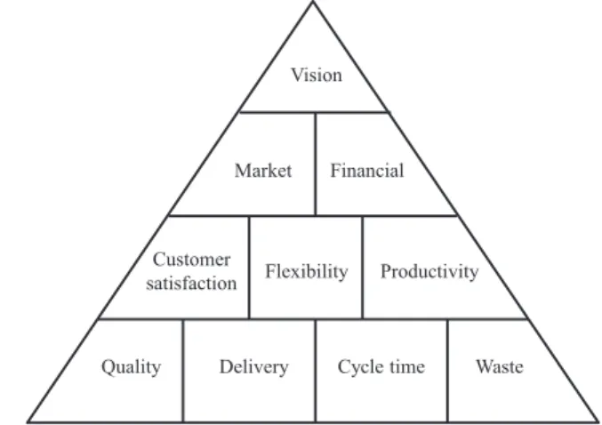
firm’s strategic goals. Ref.[51]developed a performance pyramid
(as shown inFig. 1) that enab les to correct this weakness. Supply chain management integrates supply and demand man-agement within and across companies, and encompasses the planning and management of all activities involved in sourcing and procurement, conversion, and all logistics management activities
[43]. Based on this statement, the criteria for measuring the perfor-mance of a supply chain (SC) can b e grouped into three categories: those associated with the performance of the upstream activities of the SC (with respect to sourcing and procurement), those used to measure the performance of the internal SC (with respect to conver-sion or manufacturing operations), and those used to measure the performance of the downstream activities (with respect to deliv-ery), as well as the logistics component of the SC, with the aim of satisfying the customer. The performance measures and metrics
Quality Delivery Cycle time Waste Vision
Market Financial
Customer
satisfaction Flexibility Productivity
Fig. 1. Performance pyramid. Source: Ref.[51].
Table 2
Determining factors of the tactical planning SCOR processes.
1. Determinants of the plan process
1.1 Planning horizon - Short (monthly) - Medium (quarterly) - Long (yearly) 1.2 Frozen time fence - Short (some days)
- Medium (some weeks) - Long (some months) 1.3 Time b ucket - Short (1 day)
- Medium (1 week) - Long (1 month) 1.4 Cycle time - Short (some days)
- Medium (some weeks) - Long (some months) 1.5 Non-frozen interval - Liquid order policy
- Slushy order policy 2. Determinants of the source process
2.1 Lot sizing (replenishment policy)
- Fixed order quantity - Fixed period quantity - Period order quantity - Lot-for-lot
2.2 Inventory policy (materials availab ility)
- Low safety stock - Medium safety stock - High safety stock 2.3 Procurement lead time - Short (some days)
- Medium (some weeks) - Long (some months) 3. Determinants of the make process
3.1 Capacity management policy - Constant output rate - Chase demand - Mixed strategy 3.2 Lot sizing (production quantity
policy)
- Fixed b atch quantity - Fixed period quantity - Lot-for-lot
3.3 Inventory policy (work-in-process policy)
- Low safety stock - Medium safety stock - High safety stock 3.4 Production lead time - Short (some days)
- Medium (some weeks) - Long (some months) 3.5 Scheduling - Forward
- Backward 3.6 Sequencing - Earliest Due Date
- First In, First Out - Last In, First Out - Shortest Processing Time - Longest Processing Time - Critical ratio
4. Determinants of the deliver process 4.1 Lot sizing (delivery order quantity)
- Fixed order quantity - Fixed period quantity - Period order quantity - Lot-for-lot
4.2 Inventory policy (end-product availab ility)
- Low safety stock - Medium safety stock - High safety stock 4.3 Delivery lead time - Short (some days)
- Medium (some weeks) - Long (some months) 4.4 Forecast accuracy - Low confidence
- Medium confidence - High confidence
used in this paper b elong to the last category since order fulfilment is considered a component of the delivery and logistics function.
The aim of the delivery and logistics function is to ensure that the right product is delivered in the right quantity, at the right time, in the right condition (quality), to the right place, with the right documents, and for the right cost[2,52,53]. Possib le correspond-ing performance metrics (or measures) are: delivery item accuracy for right product, delivery quantity accuracy for right quantity, on-time delivery for right time, quality conformance for right con-dition, delivery location accuracy for right place, documentation accuracy for right document, and delivery efficiency for right cost.
Based on the performance pyramid (Fig. 1) of Ref.[51], we can
say that these seven performance metrics constitute the quality and delivery performance measures that lead to customers’ satis-faction, which in turn contrib utes to higher market and financial performance, thereb y achieving the firm’s strategic goals in terms of efficiency and effectiveness. In support of this statement, some
authors[54,55]suggest that customer satisfaction implies lower
marketing costs, less price elasticity, and higher customer loyalty, which in turn lead to improvements in financial performance meas-ures such as sales revenue and market share.
2.3. Impact of tactical supply chain planning determinants on performance
In extant literature, contrib utions on the impact of tactical sup-ply chain planning determinants (TSCPDs) on performance are very diverse in scope and nature, and most often remain dispersed. Some studies focus on internal job shop performance metrics such as average lateness, average flow time, average tardiness, proportion of tardy job s, maximum lateness/tardiness, machine utilisation,
and work-in-process inventory [56,57]. Ref. [58] reported that
reducing the lot size reduces the fraction of defective products.
Ref. [59] studied assemb ly line sequencing prob lems with the
aim of minimising tardiness cost, as well as some other internal performance measures such as costs related to setup, production rate variation, operator idleness, operator error and utility worker. Regarding the authors that looked at the external performance measures, most of the studies focus on the impact of only one or a few determinants (from only one supply chain function – plan, source, make or deliver) on one or a few performance measures.
For example, Ref.[60]found that the lengthening of the planning
horizon always reduces the glob al cost. Ref.[61]looked at the rela-tionship b etween lot size, lead time, inventory, and performance.
Moving a step further, a few authors have studied the impact of a comb ination of two or more planning determinants on per-formance measures, b ut the studied determinants still b elong to the same supply chain function (plan, source, make or deliver).
For example, Ref.[62]reported that simultaneously reducing setup
times and lot sizes was found to b e the most effective way to cut inventory levels and improve customer service. Here, b oth setup times and lot sizes b elong to the make (manufacturing) function. After studying the effects of four determinants (capacity, storage time, scheduling and sequencing rules, all b elonging to the make function) on the performance of a specific two-stage system, Ref.
[13]concluded that, contrary to common sense in operations
man-agement, the Longest Processing Time sequencing rule is ab le to
maximise the total production volume per day. Ref.[63]
investi-gated the effectiveness of a tactical demand-capacity management policy to guide decisions in order-driven production systems and found that the dynamic capacity allocation procedure produces higher profit compared to a first-come-first-served policy. Look-ing at the demand side of a supply network in a configure-to-order
environment, Ref.[64]studied the impact of three factors (demand
that all the three variab les individually and interactively influence customer service performance.
Ref.[42]studied eight factors (non-frozen interval policy, plan-ning horizon length, frozen interval length, re-planplan-ning frequency, cycle length, vendor flexib ility, demand range and demand lumpi-ness) and arrived at the conclusion that vendor flexib ility and its interactions with Master Production Schedule design factors are the most significant drivers of system performance in two-stage supply chains. Though this study considers determinants from different supply chain functions, it investigates their impact only on internal performance measures. In this paper, we are rather interested not only in comb ining determinants from different supply chain func-tions, b ut also in studying their impact on external performance
measures as defined in Section2.2.
Therefore, b eyond the aim of looking at the impact of one or a few TSCPDs on one or a few performance measures, our study constitutes a significant contrib ution given that it adopts an inte-grated approach that explicitly analyses the impact of many TSCPDs from different supply chain functions on many (most important) external performance measures. With reference to supply chain
planning in the forest products industry, Ref. [21] stated that
procurement, production and distrib ution activities are always b ounded b y the trade-offs b etween yield, logistical costs and service levels. Based on this statement, we formulate our research hypothesis as:
Different combinations of tactical planning determinants from two or more supply chain functions (plan, source, make or deliver) would impact differently on a given set of external performance measures.
This hypothesis can b e reformulated as a research question in the following manner:
What combination of tactical supply chain planning determinants would enable to optimise supply chain performance, given the possible trade-off between different performance measures?
3. Methodology and numerical application
To address our research question, this paper starts b y propos-ing an integrated framework that incorporates the determinants of all the four SCOR process areas (plan, source, make, and deliver), as well as the customer order decoupling point (CODP) concept. The CODP is defined b y some authors as the point in the goods flow where forecast-driven production and customer-driven
pro-duction/delivery are separated[65]. This framework is shown in
Fig. 2.
As can b e seen in Fig. 2, there are three supply chain
con-figurations – make-to-stock (MTS), make-to-order (MTO) and assemb le-to-order (ATO). In the MTS system, the deliver process is downstream of the CODP and therefore demand-driven, while the source and make processes are upstream of the CODP and therefore forecast-driven. In the MTO system, the make and deliver processes are downstream of the CODP and therefore demand-driven, while the source process is upstream of the CODP and therefore forecast-driven. The ATO system is a hyb rid system that is mid-way b etween the MTS and MTO systems. In this system, the deliver process and part of the make process (the final assemb ly of products) are down-stream of the CODP and therefore demand-driven, while the source process and the other part of the make process (the fab rication of semi-finished products) are upstream of the CODP and therefore forecast-driven.
Based on this integrated framework we propose a five-step decision-making methodology that would enab le the planning manager to optimise SC performance b y identifying the b est com-b ination of TSCPDs. The five steps are descricom-b ed as follows. Step 1: Identify all the planning determinants of the four SCOR
process areas (plan, source, make and deliver) and
shortlist the most important, taking into consideration the type of production system (make-to-stock, assemb le-to-order or make-to-le-to-order). Then, define the values of the selected determinants b ased on the characteristics of the supply chain.
Step 2: Identify all performance measures that are in line with the firm’s strategic goals and b usiness environment, and then determine the key performance metrics with respect to the ob jectives of the supply chain.
Step 3: Identify and choose a modelling/simulation method. See
Ref.[22]for a comprehensive review of planning models
and techniques that are applied to different supply chain configurations.
Step 4: Develop the optimisation (or decision-making) model, run simulations, and perform some sensitivity analyses. Step 5: Identify the strongest and weakest comb inations of
planning determinants b y analysing their impact on per-formance. Then, choose the b est (optimal) comb ination of planning determinants.
To illustrate how the proposed methodology can b e applied to a given supply chain configuration, we will start b y describ ing the supply chain that we studied, b efore presenting the five steps. 3.1. The supply chain
In their review of integrated production-distrib ution (P-D)
plan-ning models and techniques, Ref. [22] grouped the identified
models into seven categories: 1. Single-product P-D models.
2. Multiple-product, single-plant P-D models.
3. Multiple-product, multiple-plant, single or no warehouse P-D models.
4. Multiple-product, multiple-plant, multiple-warehouse, single or no end-user P-D models.
5. Multiple-product, multiple-plant, multiple-warehouse,
multiple-end user, single-transport path P-D models.
6. Multiple-product, multiple-plant, multiple-warehouse,
multiple-end user, multiple-transport path, no-time period P-D models.
7. Multiple-product, multiple-plant, multiple-warehouse,
multiple-end user, multiple-transport path, multiple-time-period P-D models.
The case study used in this paper can b e likened to category 3 (multiple-product, multiple-plant, single or no warehouse P-D models) of their classification. In essence, it is a two-stage and two-product supply chain in a make-to-stock environment where
production is planned b ased on demand forecasts (seeFig. 3). The
two product groups (shelves and tab les) are produced and deliv-ered to end customers. The product structures of the two product groups are simple, with one component at each level. Each pro-duction plant in the supply chain makes just one component. The first plant (sawmills) transforms and delivers wooden parts (tab le legs, tab le trays and shelf b oards) to the assemb ly plant that con-stitutes the second and final production stage for the shelves. After assemb ly, tab les are shipped to a third plant for the painting oper-ation. The sawmills, the assemb ly plant and the painting shop are assumed to collab orate in a dyadic supplier-customer relationship. Each plant is considered to b e a single resource with limited capac-ity. Regarding the supply of raw materials, we assume an ideal situation – constant, regular, and without shortage.
Transportation is required b etween any two plants. Activi-ties and resources needed for transportation are lumped together such that each transport operation is characterised b y a given
Supply chain
Source Make Deliver Plan
- Capacity policy - Work-in-process -Lot sizing -Production lead time - Scheduling - Sequencing - Replenishment policy
- Procurement lead time - Material availability
- Delivery order quantity - Delivery lead time - End product availability - Forecast accuracy -Planning horizon
-Time bucket - Frozen time fence -Non-frozen interval - Cycle time
Performance measures - Delivery item accuracy - Delivery quantity accuracy - On-time delivery - Quality conformance - Delivery location accuracy - Documentation accuracy - Delivery efficiency (cost)
Demand-driven order delivery MTS CODP ATO CODP MTO CODP Suppl y pe rsp ecti ve C usto me r pe rsp ecti ve Demand-driven final assembly and customer order delivery Demand-driven fabrication, final assembly and customer order delivery Forecast-driven
procurement, fabrication and final assembly
Forecast-driven procurement Forecast-driven Procurement and fabrication
Fig. 2. Integrated tactical supply chain planning determinants b ased on the SCOR model.
capacity (limiting transfer throughput) and a lead time. Each plant is solely responsib le for managing its processes – procurement, pro-duction, storage and delivery. We assume that the lead time for the transmission of information is zero.
3.2. Application of the proposed five-step methodology Step 1: Identifying and selecting planning determinants
The framework shown inFig. 2serves to identify and select the
most relevant determinants for a given supply chain configuration. In this framework, the customer order decoupling point (CODP) is used to distinguish three supply chain configurations: make-to-stock (MTS), assemb le-to-order (ATO) and make-to-order (MTO).
Ref.[66]defined the CODP as the point in the value-adding material
flow that separates decision made under uncertainty from deci-sions made under certainty concerning customer demand. Based on this definition, we can say that the most relevant tactical plan-ning determinants for a given supply chain configuration depend
on the one hand on the type of production system – MTS, ATO or MTO (see Ref.[67]for detailed information on the factors that deter-mine the strategic positioning of the CODP) and on the other hand on the factors of uncertainty emb edded in the supply chain and its environment.
In MTS systems, b ased on the forecast of future orders, finished products are produced in advance and kept in inventory, which is then used to fulfil customer orders. This implies that forecast accuracy and end-product availab ility are determinants that would have a significant impact on the customer order fill rate. In MTO systems, given that production is triggered upon the receipt of a real order from the customer, the primary challenge is how to
meet the promised delivery lead time[17,59]. In this case,
meet-ing the promised lead time will largely depend on the procurement
and capacity management policies[17,68]. Regarding ATO systems,
part of production (the final assemb ly) is triggered upon the receipt of a real customer order, while the other part (procurement and the fab rication of semi-finished products) is carried out b ased on
Table 3
Sources of uncertainty.
Uncertainty group Factors of uncertainty Description Internal organisational
uncertainty
Product characteristics Product life cycle, packaging, perishab ility, mix, or specification. Process/manufacturing Machine b reakdowns, lab our prob lems, process reliab ility, etc. Control/chaos/response uncertainty Uncertainty as a result of control systems in the supply chain.
Decision complexity Uncertainty that arises b ecause of multiple dimensions in decision-making process, e.g. multiple goals, constraints, long term plan, etc.
Organisation structure and human b ehaviour
E.g. organisation culture.
IT/IS complexity The realisation of threats to IT use in the application level, organisational level and inter-organisational level, e.g. computer viruses, technical failure, unauthorised physical access, misuse, etc.
Internal supply chain uncertainty
End customer demand Irregular purchases or irregular orders from final recipient of product or service.
Demand amplification Amplification of demand due to the b ullwhip effect.
Supplier Supplier performance issues, such as quality prob lems, late delivery, etc. Parallel interaction Parallel interaction refers to the situation where there is interaction b etween
different channels of the supply chain in the same tier.
Order forecast horizon/lead-time gap The longer the horizon, the larger the forecast errors and hence there is greater uncertainty in the demand forecasts.
Chain configuration, infrastructure and facilities
E.g. numb er of parties involved, facilities used or location, etc.
External uncertainties Environment E.g. political, government policy, macroeconomic and social issues, competitor b ehaviour.
Disruption/natural uncertainties E.g. earthquake, tsunamis, non-deterministic chaos, etc. Source: Ref.[69].
forecast. Therefore, key determinants in ATO systems would include the key determinants of MTS and MTO systems.
Regarding the degree of uncertainty of the supply chain, Ref.[69]
reviewed the extant literature and identified fourteen sources of uncertainty, which they divided into three groups – internal organi-sation uncertainty, internal supply chain uncertainty and external uncertainty – as shown inTab le 3.
The further the CODP is positioned downstream the more the value-adding activities would b e carried out under uncertainty. On the contrary, the more the CODP is positioned upstream, the more the value-adding activities would b e carried out under cer-tainty[66]. It follows that the tactical planning determinants to b e considered in a given supply chain configuration would depend on the factors of uncertainty that are downstream or upstream of the CODP. For example, in MTS systems, tactical planning determinants would b e sub ject to most of the internal organisation and internal supply chain uncertainty factors since the procurement, fab rication and final assemb ly activities are upstream of the CODP. However, the selection of the relevant planning determinants would depend on the degree of uncertainty, as well as on the consequences of the uncertainty.
Regarding the supply chain that is used as a case study in this paper, we identified six tactical supply chain planning determi-nants (TSCPDs): two (frozen time fence and cycle time) from the plan process area, two (capacity management policy and sequenc-ing) from the make process area, and two (end-product availab ility and forecast accuracy) from the delivery process area. End-product availab ility and forecast accuracy are chosen since the studied sup-ply chain is an MTS system. For the make process area, we chose to simulate capacity management policy and sequencing since each manufacturing plant is considered to b e a single resource with limited capacity. Limited capacity would lead to either shortage or excess inventory following an increase or a decrease in demand
forecast. In this case, finding the right sequencing in a multi-products system would b e a crucial issue. Consequently, cycle times will depend on sequencing, and to ob tain the b est capacity man-agement performance, the frozen time fence has to b e optimised. We note that no determinant is chosen from the source process area since we assumed that raw materials are supplied in an ideal situation – constant, regular, and without shortage.
Frozen time fence is simulated b y considering different values (T = 5 or 10 periods) for the period of replenishment T. In this case, the decision making process is dynamically depicted according to the principle of rolling planning horizon. Two cycle times (long and
short) are simulated. The transportation lead time stated inTab le 4
represents values corresponding to a long cycle time. In this case, transportation cost is assumed to b e low (0.03). A short cycle time is 50% of the long cycle time and implies reducing the transportation lead time b y 50%. The transportation cost is therefore higher (0.1). Two capacity policies are considered for each partner – the “constant output rate” strategy where the production rate is equal to the average demand over the planning horizon, and the “chase demand” strategy in which manufacturing capacity is var-ied according to demand. We note that the first strategy entails reducing the initial production cost (80% of the nominal cost given in Tab le 4) whereas in the second strategy, production cost is increased (150% of the nominal cost). We studied two sequencing rules: first-in-first-out (FIFO) where b acklogs are processed first b efore the most recent or incoming customer orders, and last-in-first-out (LIFO), which gives higher priorities to the most recent orders.
Materials or end product availab ility (or inventory policy) is expressed in terms of safety stock. Two cases are tested: with or without safety stock. Without safety stock means that the param-eter SSr
pis set to zero. Otherwise, the safety stock is evaluated with the formula: SSr
p= K!pr √
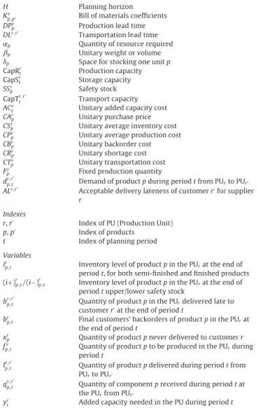
Table 4 Model notations.
Parameters
H Planning horizon Kr
p,p′ Bill of materials coefficients
DPr
p Production lead time
DLr,r′
Transportation lead time ˛p Quantity of resource required
ˇp Unitary weight or volume
ıp Space for stocking one unit p
CapRr t Production capacity CapSr t Storage capacity SSr p Safety stock CapTr,r′ t Transport capacity ACr
t Unitary added capacity cost
CAr
p Unitary purchase price
CSr
p Unitary average inventory cost
CPr
p Unitary average production cost
CBr
p Unitary b ackorder cost
CRr
p Unitary shortage cost
CTr
p Unitary transportation cost
Fr
p Fixed production quantity
dr,r′
p,t Demand of product p during period t from PUrto PUr′
ALr,r′
Acceptab le delivery lateness of customer r′for supplier
r Indexes
r, r′ Index of PU (Production Unit)
p, p′ Index of products
t Index of planning period Variables
ir
p,t Inventory level of product p in the PUrat the end of
period t, for b oth semi-finished and finished products (i+)r
p,t/(i− )rp,t Inventory level of product p in the PUrat the end of
period t upper/lower safety stock br,r′
p,t Quantity of product p in the PUrdelivered late to
customer r′at the end of period t
br
p,t Final customers’ b ackorders of product p in the PUrat
the end of period t xr
p Quantity of product p never delivered to customer r
fr
p,t Quantity of product p to b e produced in the PUrduring
period t
lr,rp,t′ Quantity of product p delivered during period t from
PUrto PUr′
qr,rp,t′ Quantity of component p received during period t at
the PUrfrom PUr′
yr
t Added capacity needed in the PU during period t
the specified service level (ab acus), !r
pis the standard deviation
of the demand in the resource r, and D represents the replenish-ment lead time. D can b e transportation lead time for materials or production lead time for end products. Finally, two situations of forecast accuracy are simulated: a fairly accurate forecast where actual demand varies only slightly with respect to forecasts and a low confidence forecast where actual demand is sub jected to huge variations compared to the forecasts.
Step 2: Identifying and determining performance measures and metrics
In Section2.2, we identified seven performance measures for an order fulfilment process: delivery item accuracy, delivery quantity accuracy, on-time delivery, quality conformance, delivery loca-tion accuracy, documentaloca-tion accuracy and delivery efficiency. In the case of the supply chain that we studied, four of these measures (delivery item accuracy, quality conformance, delivery location accuracy, and documentation accuracy) are considered to b e second-order performance measures since a high or low performance on these parameters would impact the other three measures. For example, the delivery of defective or wrong products at a wrong location and with incomplete (or wrong) documents would negatively impact on cost and on-time-delivery of the right products. We have therefore simulated only three measures
(delivery efficiency, delivery quantity accuracy, and on-time deliv-ery), which we consider as first-order measures. These three
performance measures are mentioned b y Ref.[70]as the primary
goal of supply chain planning. In this paper, they are defined in the following manner:
• Delivery efficiency is measured in terms of profit margin. An effi-cient system aims to minimise cost, thereb y maximising profit. In this study, we normalised this metric b y taking the highest profit as 100% and then calculating the others with respect to it. • Delivery quantity accuracy is measured in terms of the
percent-age of ordered quantities that are delivered within a given time frame. SRp,r′,r=
!
Hl r,r′ p,t!
Hd r,r′ p,t (1) Its value goes from 0 to 100%, the latter b eing the b est. 0% means that nothing is delivered on time and 100% means that all the ordered quantities are delivered on time. We will refer to this metric as “Completeness”.• On-time delivery is measured as the Normalised Average Delivery Time (NADT) of the total quantity that is delivered.
NADTp,t,r′,r=
!
ALr,r′ i=0 AL r,r′− i ALr,r′ l r,r′ p,t+i dr,rp,t′ (2)where ALr,r′is the acceptab le delivery lateness of customer r′from supplier r. For all quantity delivered on time (on the due date), AL = 100% and for those delivered after the period of acceptab le delivery lateness, AL = 0.
For example, let us consider an order of 10 units of a product to b e delivered on day 1 (due date), with a maximum acceptab le lateness of 3 days b eyond the due date. If 3 units are delivered on day 1, 3 on day 2, 1 on day 3, 1 on day 4, and 2 on day 5, on-time delivery is equal to 60%. This is ob tained b y calculating the NADT as follows:
NADT = [(3 × 1) + (3 × 0.75) + (1 × 0.5) + (1 × 0.25) + (2 × 0)]10 × 100% = 60%
Being normalised, the value of NADT must b e b etween 0 and 100%, the latter b eing the b est. A value of 100 means that 100% of the ordered quantity was delivered on or b efore the due date; a value close to 100 signifies that a high percentage of the ordered quantity was delivered on or b efore the due date and/or that most of the delivery was done (quickly) on the first day after the due date; while a value close to 0 signifies that most of the deliv-ery was done (lately) on or after the last day of the period of the acceptab le delivery lateness.
Step 3: Choosing a model
In the operations management literature, there are two types of models:
• Analytical models (deterministic or stochastic), which are used to study the b ehaviour of a supply chain using a mathematical approach[71].
• Simulation models, which are used in analysing complex systems
whose state changes with time and/or in a random manner[72]
and where analytical models are not easy to apply since they require strong assumptions in order to reduce complexity.
Given the holistic and integrated (complex) nature of our study, we will use the simulation approach to study the impact of the tactical planning determinants on performance. However, we will
first use a deterministic analytical approach to model the system b ecause analytical models make it easy to see the time horizon as a set of time periods, as used in planning approaches especially for rolling horizon experiments. In our model, the simulation of the planning decision-making process performed b y each partner (also called Production Unit and noted PU) in the supply chain is done b y solving a generic linear programming model.
Step 4: Model development and simulation
The proposed model defines optimal plans under storage, production and transportation capacity constraints. Prior to for-mulating the mathematical model that enab les to determine an optimal plan, the following assumptions are made: (1) each PU is associated to one resource r and manufactures a set of products p, (2) each resource has an inb ound inventory of components and an outb ound inventory of semi-finished or finished products, (3) sup-pliers of supsup-pliers are considered as very reliab le, with complete and on-time deliveries, and (4) b ackorders concern only products delivered to end customers. The notations used to describ e the
model are summarised inTab le 4.
The model plans production, inventory levels, replenishment and delivery according to customers’ orders. The ob jective function is a cost function that aims to minimise costs related to produc-tion, inventory, purchasing, shortages (orders that are considered not to have b een delivered at the end of the customer’s acceptab le delivery lead time) and b ackorders (late deliveries).
min Cf =
"
t#
"
r′"
r"
p (qr,r′ p,t· CArp) +"
r#
"
p′ ((i+)r p′,t+ 5 · (i− )rp′,t) · CSpr′+"
p (fr p,t· CPpr+ brp,t· CBrp+ Xpr· CRrp+ lrp,t· CTpr) + yrt· ACtr$$
(3)The ab ove ob jective function is solved sub ject to 7 constraint functions as follows.
Eqs.(4a) and (4b )represent the evolution of inventory levels. Eq.
(4a)concerns the finished products: the quantity resulting from the
production at a period t corresponds to a production order released a few periods b efore (depending on the production lead time DP). Eq.(4b )evaluates the inventory levels of each component according to the quantities received b y suppliers and quantities consumed b y production, b ased on coefficients in the b ill of materials. Given that in a supply chain, the end product of a production unit b ecomes a component for the downstream production unit, we use the same index p for b oth components and finished products. Therefore, in Eq.(4a), ir
p,tmeans inventory level of finished product p in
produc-tion unit r at the end of period t, whereas in Eq.(4b ), ir p,t stands for the inventory level of component (product) p in the production unit r at the end of period t.
ir p,t= irp,t− 1+ fp,t− DPr r p−
"
r′ lr,rp,t′,∀
p, t, r (4a) ir p,t= irp,t− 1+"
r′ qrp,t′,r−"
p′ (Kr p,p′× fpr′,t),∀
p, t, r (4b )Eq.(5)expresses b ackorders, that is, the difference b etween the
quantity ordered b y customers and the quantity actually delivered. br,rp,t′= br,rp,t− 1′ + drp,t′,r− lr,r
′
p,t − xr,r
′
p,t,
∀
p, t, r, r′ (5)Eqs. (6a), (6b ) and (6c) represent respectively capacity restric-tions for production, inventory and transportation. The use of an
additional capacity for production is allowed b ut requires higher operational costs.
"
p⎛
⎝
˛p· DPr p"
"=1 fr p,t− "+1⎞
⎠
≤ CapRrt+ yrt,∀
t, r, r′ (6a)"
p ∈ Pr ıp· irp,t≤ CapSr,∀
t, r, r′ (6b )"
p ∈ ˆPr ˇp· lr,rp ′≤ CapTr,r′,∀
t, r, r′ (6c)Eq.(7)represents the upper b ound of the additional capacity.
Yr
t ≤ CAPSUPP,
∀
p, t, r (7)Eqs.(8a) and (8b )represent the lower and upper b oundaries of the safety stock threshold.
(i+)r
p,t− (i− )rp,t= irp,t− SSpr,
∀
p, t, r (8a)(i− )r
p,t≤ SSpr,
∀
p, t, r (8b )Eq.(9)is activated only if the state of the capacity policy determi-nant corresponds to “constant output rate” (entire COR = 1). In this case, the material flow is fixed as the mean value of the production capacity.
(fr
p,t= Fpr)
∀
p, t, r (9)Finally, Eq.(10)corresponds to the non-negativity constraints for
all the variab les.
qr,rp,t′, irp,t, (i+)rp,t, (i− )r p,t, br,r ′ p,t, lr,r ′ p,t, yrt≥ 0,
∀
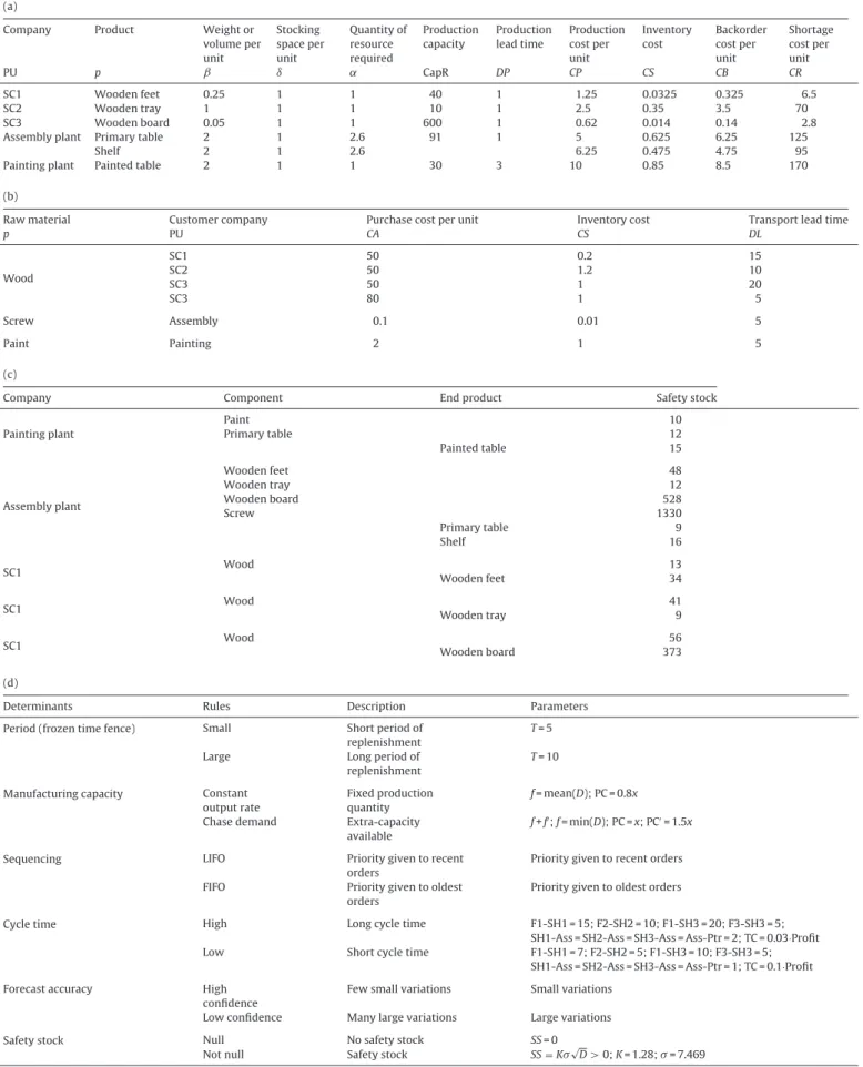
p, t, r (10)The data used for the simulation are presented inTab le 5.
Concerning the suppliers, their production lead time is included in the transportation lead time and they have no b ackorders. For all the supply chain partners, the additional production capacity (addi-tional capacity) is infinite and its unit cost is 50% higher than that of the normal capacity. For each of the companies, the inventory capacity is equal to 5000 units, the delivery transportation capac-ity is 3000 units per period and the transportation lead time is 1 or 2 periods depending on the cycle time (short or long).
Each simulation runs in a rolling horizon of 40 periods, with specific parameter values for the tested determinants – two pos-sib le states for each determinant. Each comb ination corresponds to one simulation scenario. By changing the value of one deter-minant at a time we performed 64 simulations. These simulations enab led us to assess the impact of the six determinants (frozen time fence, cycle time, capacity policy, sequencing, materials availab il-ity, and forecast accuracy) on the three performance metrics (profit margin, completeness, and NADT). The profit margin, NADT and completeness were determined for each of the supply chain part-ners. The total values for each of these three performance metrics were computed for the whole supply chain. For the sake of sim-plicity, we will not present the details for each plant, b ut only the total values: total profit, total NADT for shelves, total complete-ness for shelves, total NADT for tab les and total completecomplete-ness for tab les. Also, given the high numb er of simulations performed, we consider that a sensitivity analysis in not necessary since different values of the determinants are tested in the various comb inations.
Table 5 Simulation data.
(a)
Company Product Weight or volume per unit Stocking space per unit Quantity of resource required Production capacity Production lead time Production cost per unit Inventory cost Backorder cost per unit Shortage cost per unit PU p ˇ ı ˛ CapR DP CP CS CB CR SC1 Wooden feet 0.25 1 1 40 1 1.25 0.0325 0.325 6.5 SC2 Wooden tray 1 1 1 10 1 2.5 0.35 3.5 70 SC3 Wooden b oard 0.05 1 1 600 1 0.62 0.014 0.14 2.8 Assemb ly plant Primary tab le 2 1 2.6 91 1 5 0.625 6.25 125
Shelf 2 1 2.6 6.25 0.475 4.75 95 Painting plant Painted tab le 2 1 1 30 3 10 0.85 8.5 170 (b )
Raw material Customer company Purchase cost per unit Inventory cost Transport lead time
p PU CA CS DL Wood SC1 50 0.2 15 SC2 50 1.2 10 SC3 50 1 20 SC3 80 1 5 Screw Assemb ly 0.1 0.01 5 Paint Painting 2 1 5 (c)
Company Component End product Safety stock Painting plant Paint 10 Primary tab le 12 Painted tab le 15 Assemb ly plant Wooden feet 48 Wooden tray 12 Wooden b oard 528 Screw 1330 Primary tab le 9 Shelf 16
SC1 Wood Wooden feet 1334
SC1 Wood Wooden tray 419
SC1 Wood Wooden b oard 37356
(d)
Determinants Rules Description Parameters Period (frozen time fence) Small Short period of
replenishment
T= 5 Large Long period of
replenishment
T= 10 Manufacturing capacity Constant
output rate
Fixed production quantity
f= mean(D); PC = 0.8x Chase demand Extra-capacity
availab le f+ f
′; f = min(D); PC = x; PC′= 1.5x
Sequencing LIFO Priority given to recent orders
Priority given to recent orders FIFO Priority given to oldest
orders
Priority given to oldest orders
Cycle time High Long cycle time F1-SH1 = 15; F2-SH2 = 10; F1-SH3 = 20; F3-SH3 = 5; SH1-Ass = SH2-Ass = SH3-Ass = Ass-Ptr = 2; TC = 0.03·Profit Low Short cycle time F1-SH1 = 7; F2-SH2 = 5; F1-SH3 = 10; F3-SH3 = 5;
SH1-Ass = SH2-Ass = SH3-Ass = Ass-Ptr = 1; TC = 0.1·Profit Forecast accuracy High
confidence
Few small variations Small variations Low confidence Many large variations Large variations Safety stock Null No safety stock SS= 0
1... 2... 3... 4... 5... 6... 7... 8... 9... 10... 11... 12... 13... 14... 15... 16... 17... 18... 19... 20... 21... 22... 23... 24... 25... 26... 27... 28... 29... 30... 31... 32... 33... 34... 35... 36... 37... 38... 39... 40... 41... 42... 44...45...43... 46... 48...47... 49... 50... 51... 52... 53... 54... 55... 56... 57... 58...60...61..59... . 62...64...63... Profit margin NADT Shelve Compl. Shelve NADT Table Compl. Table Axe 1 (45 .99%) Axe 2 (21 .99%) Cluster 1 Custer 2 Cluster 3 Cluster 4 Cluster 5
ClustersGood Bad Good Bad Good Bad Good Bad Good Bad
Cluster 1 X X X X
Cluster 2 X X X X
Cluster 3 X X X X
Cluster 4 X X X X
Cluster 5
CompletessTables' performanceNADT Shelves' performance
Whole SC
No significative discrimination
Profit Margin Completess NADT
No preponderan
t criteria
Fig. 4. PCA factorial plan and cluster analysis.
Moreover, sensitivity analyses would b e more valuab le in a real world b usiness application with real data.
Step 5: Analysis of the simulation results and decision making Given that this paper aims to explain the relationship b etween comb inations of determinants (simulation scenarios) and perfor-mance measures (simulation results), we have chosen to use the Principle Component Analysis (PCA) to analyse our results since it enab les to highlight key quantitative variab les that explain the major quantitative differences b etween the simulation scenarios (especially the effect of scale). A glob al analysis was performed in order to define clusters of the performance results of the simulation scenarios. Based on this, we assessed the common characteristics of the scenarios that composed a cluster in order to highlight the key determinants that can explain the differences b etween the clusters. In other words, a PCA was carried out on the whole of the numer-ical variab les used in our study: 64 simulations and 5 characters (profit, completeness for tab les, NADT for tab les, completeness for shelves, and NADT for shelves). As can b e seen inTab le 6, two axes
represent ab out 70% of the information and can consequently b e interpreted.
The first axis shows that the glob al profit margin character and the performances on the characters of tab les (NADT and in a lesser manner completeness) are closely related. It appears so b ecause tab les are more profitab le than shelves. If the NADT is good on this product then the profit will equally b e good. We also note that no character is really opposed to this trend. The second axis shows for shelves some discrimination b etween the simulations that have a high level of performance in terms of completeness and those that maximise the NADT performance level.
The PCA singled out five clusters as shown inFig. 4. We note that cluster no. 5 is not really significant. Its central position indicates that no character of the factorial plan allows isolating the results of the simulation from the others. In other words, cluster no. 5 con-stitutes the “weak underb elly” of our study. We therefore focus our analysis on the first four clusters.
In order to identify the effect of each determinant on the performance of the supply chain, we first analysed the detailed characteristics of each of the simulations that composed the
Table 6
PCA analysis: what the axes imply.
Axis 1 (+45.99%) Axis 2 (+21.99%)
Positive impacts Profit margin +41% Completeness: shelve +55% NADT: tab le +29% Completeness: tab le +4% Completeness: tab le +13%
Negative impacts NADT: shelve − 11% NADT: shelve − 35% Completeness: shelve − 4% NADT: tab le − 4%
clusters. Then we compared all the scenario characteristics of a cluster and associated them to the overall performance of the con-sidered cluster. Consequently, b y analysing the reasons that justify the discriminations b etween clusters no. 1, 2, 3 and 4, we clearly ob served that the determinants that have the most important effect on performance are manufacturing capacity and sequencing.
Manufacturing capacity has a strong impact on profit margin. The constant output rate strategy gives the b est profit margin whereas the chase demand strategy is associated with the worst scenarios in terms of profit margin. It means that the former enab les an optimal use of production resources. Also, inventory costs are generally lower than the production costs associated with the addi-tional capacity. Considering the six determinants that we studied, these ob servations provide a first answer to our research ques-tion. We can say that manufacturing capacity is the predominant determinant that impacts on delivery efficiency.
The sequencing determinant has a strong impact on complete-ness and NADT. In the case of the FIFO rule, completecomplete-ness increases whereas in the case of the LIFO rule, NADT increases. This can b e explained b y the fact that with the FIFO rule, the supply chain gives priority to b acklogs and consequently minimises late deliver-ies (shortages), thereb y maximising the delivery quantity accuracy of the supply chain. With the LIFO rule, the supply chain gives pri-ority to the most recent customer orders and therefore maximises the on-time delivery performance measure. We note that with the FIFO rule, the service level (expressed as completeness and NADT) is moderate for the whole population of customers while with the LIFO rule, the service level is maximised only for a sub set of customers. These ob servations constitute a second answer to our research question. In essence, among the six determinants that we studied, we can say that sequencing is the predominant determi-nant as regards to delivery quantity accuracy and on-time-delivery. All the other determinants have a limited impact on perfor-mance. However b y analysing the PCA results, we noticed several positive and negative impacts of planning determinants on dif-ferent performance metrics. For example, we ob served that a low confidence on forecast leads to poor profit margins. But, when com-b ined with the constant output strategy, this determinant does not have any impact on performance (see cluster no. 4 inFig. 4). Also, cycle time appears to b e a very significant variab le that impacts on the performance of the whole supply chain. In fact, reducing the cycle time generally induces additional costs. But in our set of sim-ulations, the PCA analysis (see cluster no. 3 inFig. 4) shows clearly that these additional costs could offset the penalties associated with a poor service level. This is the reason why practitioners should consider the cycle time as a very interesting and effective variab le for improving the performance of their supply chain. Furthermore, the safety stock parameter improves (more or less) the situation of the most critical cases (see Clusters no. 3 and 4 inFig. 4). But, if the performance results are glob ally satisfactory, then safety stock does not limit performance. In other words, safety stocks would not jeopardise b enefits if there are no significant disruptions in the supply chain. Finally, the PCA analysis does not permit to reach any significant conclusion regarding the impact of planning horizon on performance. This prob ab ly indicates that this determinant is not preponderant compared to the others.
Though the simulations in this paper are performed on only one supply chain configuration, the preliminary results enab le to validate our research hypothesis, which states that different comb i-nations of tactical planning determinants from two or more supply chain functions (plan, source, make or deliver) would impact dif-ferently on a given set of external performance measures. It follows that in tactical supply chain planning, the optimal comb ination of determinants would b e decided b ased on the desired performance of the supply chain. In the case of the supply chain that we studied in this paper, the decision would b e to lay emphasis on manufac-turing capacity, sequencing and cycle time as the preponderant and performance-sensitive determinants.
4. Conclusion
The contrib ution of this paper is threefold. Firstly, b y com-b ining the SCOR model and the CODP concept, it develops an integrated framework that would enab le researchers to study the relationship b etween tactical supply chain planning determinants and performance measures, for different manufacturing config-urations (make-to-stock, assemb le-to-order and make-to-order). Secondly, it proposes a five-step decision-making approach that would enab le managers (and computer software programmers) to choose the b est comb ination of tactical planning determinants that would lead to a good (optimal) b alance b etween conflicting performance measures. Thirdly, using a mathematical model and computer simulations, it successfully shows a numerical applica-tion of the proposed methodology.
Though Ref.[3]used the SCOR model to study the impact of
planning on performance b y evaluating each of the process areas – source, make and deliver, the authors did not detail the
determi-nants of the planning process. Using the SCOR model, Ref.[4]also
studied and confirmed a positive relationship b etween all the pro-cess areas and supply chain performance, b ut did not investigate the impact of the determinants of these process areas. The contrib u-tion of this paper is therefore unique in two aspects: (1) To the b est of our knowledge, this is the first paper that presents an exhaustive list of tactical planning determinants within an integrated frame-work; (2) It proposes and applies a methodology that enab les to investigate the relationship b etween supply chain performance and various comb inations of determinants from all the four SCOR pro-cess areas (plan, source, make and deliver). Our results show how different comb inations of tactical planning determinants impact on three different supply chain performance metrics (delivery effi-ciency, delivery quantity accuracy, and on-time delivery).
From a theoretical perspective, this framework can b e used to study and develop theories that could explain the trade-offs and mediating roles b etween planning determinants. For example, Ref.
[73]studied how one planning determinant (forecast errors) can
b e mitigated b y another determinant (lot sizing rules). With our proposed framework and methodology, similar studies can now b e carried out with many determinants at the same time. Also, the practical implication is that managers can more frequently review their planning parameters according to changes in the level of uncertainty linked to the characteristics of the supply chain, as well as to its environment.