Adaptive bit allocation for spatiotemporal subband coding using vector quazntization

Adaptive Bit Allocation for Spatiotemporal

Subband Coding Using Vector Quantization

by

Xiang Chen

Beijing, P.R.China 1982

SUBMITTED TO THE MEDIA ARTS AND SCIENCES SECTION SCHOOL OF ARCHITECTURE AND PLANNING

IN PARTIAL FULFILLMENT OF THE REQUIREMENTS OF THE DEGREE OF MASTER OF SCIENCE

AT THE MASSACHUSETTS INSTITUTE OF TECHNOLOGY June 1990

@Massachusetts Institute of Technology 1990 All Rights Reserved

Signature of the Author

'Xianig Media Arts and Sciences S ion

May 11, 1990

Certified by

... A de ...B...

Lecturer, Associate Director, Media Laboratory Thesis Supervisor

Accepted by

...

.t plAVE

Chairman Departmental Committee on Graduate Students

OF TEcHNOLS

JUL 06 1990

MIT Libraries

DISCLAIMER OF QUALITY

Due to the condition of the original material, there are unavoidable

flaws in this reproduction. We have made every effort possible to

provide you with the best copy available. If you are dissatisfied with

this product and find it unusable, please contact Document Services as

soon as possible.

Thank you.

The scanned Archives copy of this thesis contains minor

background spotting on pages. This is the best available

copy.

d

Adaptive Bit Allocation for Spatiotemporal Subband

Coding Using Vector Quantization

by

Xiang Chen

Submitted to the Media Arts and Sciences Section on May 11, 1990 in partial fulfillment of the requirements of the degree of Master of Science

at the Massachusetts Institute of Technology

Abstract

Subband coding of digital image is drawing more attention than ever before. The fundamental property of subband coding system is that the original signal is decomposed into several statistically dissimilar signals. On one hand, this decomposition constitutes the primary decorrelating mechanism, which affects the signal compression. However, it raises the problem of optimally allocating the available channel capacity among the signal components. This is more critical in coding image at low bit rate. A bit allocation algorithm based on the the statistics of source image data is developed in this thesis. The original image data is first transformed into a set of spatioltemporal subbands by using QMF filters. Then statistics are run through the subbands. According to the statistics, the bit allocation program allocates the predescribed total bits to different subbands in such a way that the total distortion in the reconstructed picture will be minimized. A bit rate controlled kd-tree based vector quantizer is used to conduct the quantization.

Thesis Supervisor: Andy Lippman

Title: Lecturer, Associate Director, Media Laboratory

Work reported herein is supported by a contract from the Movies of the Future consortium, includ-ing AT&T, Columbia Pictures Entertainment Inc., Eastman Kodak Co., Paramount Pictures Inc., Viacom International Inc., and Warner Brothers Inc.

Contents

1 Introduction 13

1.1 Noiseless Source Coding . . . . 16

1.2 Noise Source Coding . . . . 17

2 Subband Coding 21 2.1 Subband principles . . . . 22

2.1.1 Subband Analysis & Synthesis . . . . 26

2.1.2 Subband Characteristics . . . . 35

2.2 Vector Quantization... . . . . 39

2.2.1 An Overview on VQ . . . . 42

2.2.2 Tree Based VQ Codebook Design . . . . 44

2.2.3 Bit Rate Control in Tree Based Codebook Design . . . . 49

3 Psychophysics and Application in Subband Coding 3.1 Psychophysics in Image Coding ...

3.2 HVS Based Bit Allocation .... ...

4 Bit Allocation & Pre-filtering

4.1 Bit Allocation ... ...

4.1.1 A Bit Allocation Algorithm development . . . . 4.1.2 Experiments on Bit Allocation . . . . 4.2 Pre-filter Issues in Image Coding . . . . 4.2.1 Prefiltering . . . .. . . . 4.2.2 Picture Quality vs. Prefiltering . . . .

5 Coding Experiments

5.1 A Coding System with Adaptive Bit Allocation - An Overview 5.2 Coding Exam ples . . . .

6 Conclusions and Further Work

6.1 Suggestions for Further Work . . . . 6.2 Conclusion . . . . q 68 76 77 77 83 88 88 101 111 .111 114 124 124 126

A Acknowledgments

B Bibliography

128

i

List of Figures

2.1 Subband Coder. . . . . 22 2.2 Partitioned Luminance Spectrum. . . . . 27 2.3 Frequency domain subdivision in a typical 3 level QMF pyramid. . 28 2.4 Arbitrary M band analysis/synthesis system. . . . . 29 2.5 Top: Notched 2way band splitter. Middle: Overlapped 2way band

splitter. Bottom: Ideal band splitter . . . . 30 2.6 Aliasing as a result of decimating the pictured spectrum (top)

by a factor of 2 . . . . 31 2.7 9 tap QMF analysis/synthesis bank. Top left: Impulse response of

the low pass filter. Top right: Impulse response of the high pass filter. Bottom: Magnitude response of low pass filter (solid line) and the high pass filter. . . . . 34 2.8 The original picture from frame 6 of second 4 of alley sequence. . . 37

2.9 Pyramid decomposition of the original picture in Figure 2.8. ... 38 2.10 Histogram for original picture and LL bands. . . . . 40

2.11 Histogram for LH, HL, and HH bands of pyramid level one. . . . . . 41 2.12 Vector quantization . . . . 43 2.13 Kd-Tree: A typical kd-tree (K = 2) shown as both a binary tree (left)

and a subdivided 2 dimension space (right) . . . . 46 2.14 Entropy increasing monotonically with N in equation 2.7 increasing.

The X axis represents N and Y axis represents entropy. . . . . 55 2.15 The Original Picture of Flower Garden . . . . 61 2.16 The picture shows the error pixels of the reconstructed image from test

1 in Table 2.4. (The error image has been gainbiased by 10.) Error pixels are easily seen to concentrate in detailed regions. . . . . 62 2.17 The picture shows the error pixels of the reconstructed image from test

8 in Table 2.4. (The error image has been gainbiased by 10.) Error pixels appear more in the slowly varying intensity areas, like the trunk of the tree and the sky. Meanwhile, there are more peaky error pixels than that in 2.16. However, there are less error pixels in the area of flow ers. . . . . 63

2.18 The picture shows the error pixels of the reconstructed image of lowest

subband of the first level pyramid of the image 2.8. The parameters combination in test 1 of Table 2.1 is used with the codebook size =

3600. It shows much less error than next picture 2.19 which has the same codebook size but using the parameters combination in test 8 of Table 2.1. This proves that the parameters combination of test 1 is good for the subband with relatively flat intensity distribution. ... 64

d

2.19 The picture shows the error pixels of the reconstructed image of lowest subband of the first level pyramid of the image 2.8. The parameters combination in test 8 of Table 2.1 is used with the codebook size =

3600. It shows much more error than previous picture 2.18 which has the same codebook size but using the parameters combination in test 1 of Table 2.1. This proves that the parameters combination of test 8 is not good for the subband with relatively flat intensity distribution. 65 2.20 The picture shows the error pixels of the reconstructed image of LH

subband of the first level pyramid of the image 2.15. The parameters combination in test 1 of Table 2.1 is used with the codebook size =

1450. It shows much more obvious errors than next picture 2.21 which has the same codebook size but using the parameters combination in test 8 of Table 2.1. This proves that the parameters combination of test 1 is not good for the subband with very peaky intensity distribution. 66 2.21 The picture shows the error pixels of the reconstructed image of LH

subband of the first level pyramid of the image 2.15. The parameters combination in test 8 of Table 2.1 is used with the codebook size =

1450. It shows much less error than previous picture 2.20 which has the same codebook size but using the parameters combination in test 1 of Table 2.1. This proves that the parameters combination of test 8

is good for the subband with very peaky intensity distribution. ... 67

3.1 General Image Processing System . . . . 70

4.1 The Bit Allocation Test Result Plot . . . . 84

4.2 Labels of subbands in Figure 2.2. . . . . 86

4.3 The Bit Allocation Test for the sixth and seventh Frame of fourth S4cond of Alley Sequence with R = 0.5 . . . . 86

4.4 The Bit Allocation Test for the tenth and eleventh Frame of sixth Second of Alley Sequence with R = 0.5 . . . .. . . . . . 87

4.5 The Bit Allocation Test with R = 0.25 bits/per pixel . . . . 89

4.6 The Bit Allocation Test with R = 0.5 bits/per pixel . . . . 90

4.7 The Bit Allocation Test with R = 0.75 bits/per pixel . . . . 91

4.8 The Bit Allocation Test with R = 1.0 bits/per pixel . . . . 92

4.9 The Bit Allocation Test with R = 1.25 bits/per pixel . . . . 93

4.10 The Bit Allocation Test with R = 1.5 bits/per pixel . . . . 94

4.11 The Spectrum of a Horizontal Line of sixth frame of fourth Second from Alley Sequence. . . . . 95

4.12 Prefilters: top: filter1, second from top: filter2, second from bottom: filter3, bottom: MPEG decimation filter. . . . . 97

4.13 MPEG interpolation filter . . . . 98

4.14 Labels of 4 level pyramid subband. . . . . 98

4.15 The plot-out of energy distribution among subbands. -, -.-. , and +++ represent the image data prefiltered by filter1, filter2, and filter3, respectively. . . . . 99

4.16 The pictures in the order gf top left, top right, bottom left, bottom right represent the image prefiltered by MPEG decimation filter, filter1, filter2, filter3, respectively. . . . . 100

4.17 Diagram for Testing Prefilters . . . ... . . . . 102 4.18 The picture is prefiltered by MPEG decimation filter and down sampled

by 2. The test picture is sixth frame of fourth second of Alley sequence. 105

4 ,- ON W

4.19 The picture is prefiltered by filter3 and down sampled by 2. The test picture is sixth frame of fourth second of Alley sequence. . . . . 106 4.20 The picture is coded at 0.36 bits/per pixel. The source image data

has been prefiltered by MPEG decimation filter before being sent to the encoder. The test picture is sixth frame of fourth second of Alley sequence. ... ... 107 4.21 The picture is coded at 0.38 bits/per pixel. The source image data has

been prefiltered by filter3 before being sent to the encoder. The test picture is sixth frame of fourth second of Alley sequence. . . . 108 4.22 The picture is interpolated by 2 after being coded at 0.36 bits/per pixel.

The source image data has been prefiltered by MPEG decimation filter before being sent to the encoder. The test picture is sixth frame of fourth second of Alley sequence. . . . ... 109 4.23 The picture is interpolated by 2 after being coded at 0.38 bits/per

pixel. The source image data has been prefiltered by filter3 before being sent to the encoder. The test picture is sixth frame of fourth second of Alley sequence. . . . . 110

5.1 Image coding system with adaptive bit allocation . . . . 113 5.2 The picture is prefiltered by filter1 and downsampled by 2. The test

picture is the sixth frame of the fourth second of the Alley sequence. . 120 5.3 The picture is prefiltered by filter2 and down sampled by 2. The test

picture is the sixth frame of the fourth second of the Alley sequence. . 121 5.4 The picture is interpolated by 2 after being coded at 0.37 bits/per pixel.

The source image data has been prefiltered by filter1 before being sent to encoder. The test picture is the sixth frame of the fourth second

5.5 The picture is interpolated by 2 after being coded at 0.36 bits/per pixel. The source image data has been prefiltered by filter2 before being sent to encoder. The test picture is the sixth frame of the fourth second of the Alley sequence. . . . . 123

List of Tables

2.1 Kd-tree Parameter's Combination . . . . 53

2.2 Bits Calculation Methods Comparison . . . . 53

2.3 Kd-tree Parameters Selection Tests for Picture 2.8 . . . . 58

2.4 Kd-tree Parameters Selection Tests for Picture 2.15 . . . . 58

4.1 The Bit Allocation Test . . . . 84

4.2 Prefilter Test . . . . 103

5.1 Coding experimental results with different prefilters. . . . . 115

5.2 Coding experimental result& with MPEG decimation filter as prefilter 116 5.3 Coding experimental results with filter1 as prefilter. . . . . 117

5.4 Coding experimental results with filter2 as prefilter. . . . . 118

Chapter 1

Introduction

Digital images represented at a low enough bandwidth for them to be useful in com-puting applications and -new consungr products are more and more in demand, since both digital data communication and digital data storage are surprisingly increasing. We address image representations that allow high quality moving video sequences at near 1.5 Mb/sec.

explored the use of subband decomposition of image sequences for this purpose.

Subband coding was introduced by Crochiere et al. [34] in 1976 originally for speech coding. However, considerable attention has been devoted to subband coding of images since then. The virtue of subband coding is to split up the signal frequency band into subbands and to encode each band with a coder and bit rate accurately matched to the statistics of that particular band. Also, the response of the viewer's eye to different frequencies can be taken into account, and quantization error can be increased in those bands for which it will be less visible.

Recent advances of subband coding shows that subbands allow a multi-scale image representation [5] [40] , and afford good performance in coding [23] [1] (22].

Subband coding can be viewed in two components. First the image sequence is analyzed by a series of linear filters into spatial and temporal regions, then these re-gions are each quantized. A variety of quantizers may be used, and further processing may also be performed on the subbands. We have experimented with DCTs and VQ at the Movies of the Future Group, Media Lab, MIT (refs, tech notes, etc)

In this thesis we examine the bit allocation applied to the subbands. and the preprocessing applied to the image before subband decomposition. This is important

because the. quantization is the source of the compression, and it inherently involves a loss of data and potential reduction of picture quality. We can view this process as adding noise selectively to the image, and the manner in which the noise is add and the amount of it will determine quality and efficiency. It is important to realize that the encoding process is a matter of throwing away information (data) in such a way that the reconstructed signal at the decoder output is corrupted the least. (At least by a visual criterion, if not by a mean squared error measure.)

We will describe the basic structure of the coder and its value in compression and application, some aspects of the psychophysics of image coding that are exploited in the subband coder, and characteristics of compressed images when noise is added to the subbands. Finally, we will describe a bit allocation method and a prefilter that can be applied to the images to allow high quality and low bit rate.

Before preceding, it is worth while to briefly review Shannon's source coding theorem.

1.1

Noiseless Source Coding

A data compression system is said to be noiseless if the source symbol sequence is reproduced exactly at the destination. Consider partitioning the source sequence into subsequences of length N. We define the information contained in a source symbol sequence of length N to be

i(x) ~ log 2(p(x)) bits/source symbol. (1.1)

The average information per source symbol, known as the source's Nth order entropy is

HN(p)

-

bits

/

source

(1.2)

N gN XEx PN(X)

where pN(x) is the Nth order source pmf (probobility mass function).For most discrete sources of interest, this quantity approaches a finite limit, called its entropy, as N approaches infinity:

H(p) A lim HN(p) bits /source symbol. (1.3)

N-+oo

Theorem 1 (Shannon's Noiseless Source Coding Theorem [38]) For any e> 0, there exists a noiseless source encoder

/

The primary value of this theorem is that it provides a bound for the source coding if the source entropy is known. However, it does not give a method for constructing

a source coding system.

1.2

Noise Source Coding

When the available channel capacity is less than the source entropy, the noiseless source coding theorem implies thatwe can not communicate the source sequence without error. In this case, we can, however, try to contract a codec which introduces relatively benign types of errors in the reconstructed sequence. For such an approach, we must be able to quantify distortion between the source sequence x and the repro-duction sequence i as a function of the two sequences in a meaningful way. Ideally,

i

the distortion function should reflect the degree to which the reconstructed sequence differs from the original. So far, the most commonly employed distortion measure is the mean square error (mse), defined as

N-1

d(x, z) A N-(x(i) - i(i)) 2, (1.4) i=0

for sequences of length N. Mean square error distortion is zero in the case of perfect reconstruction.

The source coding problem is to design a codec which achieve the minimum aver-age distortion between the original and reconstructed source sequences, subject to the constraint that the average encoder output bit rate be less than a prescribed value. Alternately, we may want to minimize the average encoder output rate, subject to a constraint on the maximum allowable distortion. Here, we introduce a generalized entropy concept called rate distortion function, R(5), which specifies the minimum channel capacity required to transnit the source sequence with distortion less than

6, as stated in Shannon's Source Coding Theorem,

Theorbm 2 (Shannon's Source Coding Theorem [38] ) Fix 6 ; 6m> . For any

6' > 6 and R' > R(b), for sufficiently large N there exists a source code C of length

(a) M < 2[NR']

(b) d(C) < 6'

In this theorem, N is the number of source symbols grouped together into a block,

[-]

C = (xo,x1, ... xM-1), XJEXN. (1.5)

If we assume that the encoding function, C(.), selects the reconstruction vector i E C that minimizes the mean square error to its argument, x E xN, then the average distortion of code C is defined as

d(C) _ 1] p(x)d(x, C(x)). (1.6)

xExN

In general, R' approaches the rate distortion function only as N becomes large, im-plying that performance is proportional to the sequence length.

As we have seen, neither the noiseless nor the noisy source coding theorem provides an explicit method for constructing practical source coding systems. However, they

Chapter 2

Subband Coding

A subband coder can be viewed as two basic components as shown in Figure 2.1. The first part of the chapter discusses the subband analysis/synthesis; the virtues of subbands, such as: energy concentration, localization of features in the images, and the division of images into varying and relatively stationary subbands.

The second part of the chapter explores the kd-tree based vector quantizer; its design issues; the selection of splitting dimension and the division point on the selected

Input image

sequences Output image_sequences

Figure 2.1: Subband Coder.

dimension; and the bit rate calculation and control in kd-tree based VQ process.

2.1

Subband principles

The moving image sequences are represented as a three-dimensional digital signal with two dimensions in space and the third over time. Therefore, the three dimensional subband method should be employed to remove the redundancy in each dimension.

[44 [46] [5] [22].

In subband analysis, the input signal is broken up with a set of band-splitting filters that cover fully the frequency spectrum of the information in the original signal. Because the filters cover the frequency domain exactly and each resulting signal can be sub-sampled at its new Nyquist sampling rate, the number of data points does not

increase. However, there is a chan'ce of information loss, due to the leakage in the filters. Therefore, the desired characteristics of a subband are that its filters exhibit a minimal leakage and that the result will be a set of output subbands that have a definite hierarchy of importance. Here we need to solve two problems: finding a set of filters which preserve total information of original signal in the set of subband signals; splitting the subbands in such a way that the bandwidth of transmission channel can be intelligently allocated by more finely coding the important sub-bands and coarsely coding the unimportant ones. The Quadrature Mirror Filter (QMF) technique has been normally used as the solution for the first problem [12]. The solution for the second one is associated with issues in Human Visual System (HVS). The subband

coding schemes for image coding in conjunction with a visual model is quite strong due to the HVS's nonuniform response across different portions of the spatialtemporal spectrum. Troxel et. al. and Schreiber [42], Glenn[13] [14] and Kelly[24] all discussed the reduced distortion sensitivity to high frequency spatial detail that humans exhibit.

Spatially, the human response is not easily modeled, but there are well known components of the early visual pathway that are surprisingly well approximated us-ing simple filter banks. Butera[5] took advantage of this approach and employed a subband decomposition within an image coding system to model these components. He cites Wilson's work[45] which observes that groups of receptors in the human

vi-sual system. are organized into roughly one octave wide -circularly symmetric band pass channels. Each of these receptive units therefore responds to detail at a given scale and is isotropic in nature. This suggests a spatial subband decomposition of an image into one octave wide regions is a suitable and practical means of modeling the human visual system. It also has been shown through experimentation that humans have lower acuity with respect to diagonal edge detail than more vertical or horizontal orientations. It is important to note that source modeling alone establishes the same fact. Even though there is no universal probability distribution function for images, most of the images do not have flat spectra. In fact, the amplitude of the spectral components decreases rapidly in proportion to spatial frequency. Octave subdivisions, thereafter, make sense in that they divide the spectra into pieces which have roughly equal amounts of information.

Temporally, there is less support for octave divisions. The studies of temporal subband division are not as satisfactory as the one of spatial subband. Romano [22] described a temporal uniform subdivision scheme which uses 6Hz as base frequency. This scheme is based on the fact that 24Hz, 30Hz, and 60Hz temporal rates are widely seen in current imaging systems in this country, and all of these frequencies are conveniently divisible by 6Hz. However, the computational complexity in the implementation is very high. Lippman and Butera

[27

subband division method. In this method, there are only two temporal subbands, low and high. The low band is the average of a pair of pictures and the high band is the difference of the pair. The poor temporal resolution of the test sequences makes a further level of temporal filtering not necessary. As a matter of fact, these two temporal bands are actually composed by the shortest QMF filter. This method also gives us a perfect temporal reconstruction.

Since this thesis emphasizes the bit allocation among the subbands, choosing the coarse temporal subband division will not lose the generalization in the bit allocation problem. The bit allocation scheme developed on the two temporal subband system should be easily extended to multi-temporal subbands system.

Applying both spatial and temporal subband partitioning scheme examined above, we use a spatiotemporal system shown in Figure2.2 as the three dimensional subband model on which we will develop our ad'aptive bit allocation scheme. In the system, 1 dimensional filter is applied separately in vertical and horizontal direction to build up two dimensional spatial subband. The lowest spatial subbands of each level are further filtered to get the next level pyramid subbands. There are three levels of pyramid in all. In Figure2.2 and all of the figures throughout this thesis, we use the following notation:

* LL - Low pass filter applied both vertically and horizontally

" LH - Low pass filter applied vertically and high pass filter applied horizontally

" HL - High pass filter applied vertically and low pass filter applied horizontally

e HH - High pass filter applied both vertically and horizontally

Figure2.3 shows the corresponding diagram in frequency domain.

2.1.1

Subband Analysis & Synthesis

The problem of splitting a signal into subbands and then reconstructing it again is usually looked upon as a pure signal processing problem. The exact signal character-istics and the nature of application is not given any attention. Effectively this means that errors due to encoding, transmission and decoding are neglected. In that case the splitting and reconstruction stages become attached and the design is derected at perfect or nearly perfect reconstruction. For splitting a one dimensional signal into two subbands the QMF technique was introduced by Croisier, Esteban and Galand

LHL HH HH L7]- LHH HL LILH LH .LH iZ LLL _{LL LL} Image pair 0-LHL NoHH HH HHHH LLL L LLL LL

Temporal Vertical & horizontal Vertical & horizontal Vertical & horizontal Luminance bandsplitter 1D bandsplitter 1D bandsplitter 1D bandsplitter

t- -- - l pI II I

Tempora _{Pyramid Pyramid Pyramid}

components level one _components level two _components level three components

2

HL HH

SLLH

NH

LL i L

Lew 4 LeveI Lem 2 Lemel I

T 2i

A block diagram of an arbitrary M band system is shown in Figure2.4 The diagram

Maximally Decimated Multi-Rate Filter Bank

Coding, Transmission, and Decoding

Input _{Reconstructed}

Signal rSignal

x[n]- o - -- Hj( z ,() M M F---.VF,((n) __ _ A^n

-- & 2( z) MM -- -- F2( n

H2Z X2(n) V2(

Analysis Bank _{Synthesis Bank}

Figure 2.4: Arbitrary M band analysis/synthesis system.

implies that the M bands have equal extents, therefore, decimation rate is constant across subbands. This is not necessary. In this thesis, we set M = 2.

In traditional filter design theory, an ideal band pass filter, which seems to be required by the perfect reconstruction filter bank, is not realizable. The filters in the

real world are either separated to avoid overlap resulting in an overall notching of the

d

spectrum or. allowed to overlap resulting in aliasing. These situations are shown in Figure2.5 Neither choice satisfies the perfect reconstruction criterion.

Non-overlapping anAlysis filters

W o)

Ideal

analysis filters

Figure 2.5: Top: Notched 2way band splitter. Middle: Overlapped 2way band splitter. Bottom: Ideal band splitter

Any notch in the analysis transfer function introduces an unrecoverable error, because it completely blocks a component from passing through the system. It is therefore reasonable to allow the analysis filters to overlap resulting in aliasing and to design the whole system in such a way that the overall system make a cancellation on any aliasing. The QMF filter, which has two band, is one implementation of this idea. Figure2.6 illustrate the aliasing as a result of decimating the pictured spectrum by a factor of 2. To understand how the aliasing might be canceled through out the

overall system, let us begin by writing the expression out.

1 X(e 0)

-2m 0 2n

2

0.5[X(eJlm/2) + X (- e o /2)

Figure 2.6: Aliasing as a result of decimating the pictured spectrum (top) by a factor of 2

Analysis filters Hi (eW ) are used to decompose input x~n] into a low-frequency subband and a high-frequency subband which are in quadrature to one another. After coding, transmission, and decoding, synthesis filters Fj (ejw ) are used to reconstruct the signal. If hi (ejuj) are ideal brickwall filters. the system will obviously work without failure.

QMF's

The transfer function for the two-channel QMF bank of Figure2.4 is:

X' (ej'') 1

2

[Ho (-es'') Fo (ei'') + H1 (-ew) F1 (e')] X (-eid)

Furthermore, choosing the synthesis filters to be

Fo (e') = H1 (-e')

F1 (e') = -Ho (-ew"')

yields the overall LTI transfer function

[Ho (e') H1 (-e") - H1 (ejw) Ho (-e"')j

Adding the further constraint of

(2.1)

(2.2) (2.3)

H1 (es") = e-iw(N- 1)Ho

(-e-i")

Insures there is no aliasing, amplitude or phase distortion. For more detailed QMF design technique, see [39] or [33].

The QMF filter bank discussed above provides us the freedom in picking the optimal subdivision of the spatiotemporal spectrum to meet the requirements of the image coding system. The subdivision method used in this thesis is octave for above mentioned reasons. In this approach, each successive split cuts away half of the spectrum along a given axis as shown in Figure2.2. This spatial image decomposition is called QMF pyramid transform [1]. The QMF pyramid transform can be applied recursively to the lowest subband previous application, and the subbands from each

QMF

The 9 tap QMF analysis/synthesis bank employed in this work(designed by [39]) to perform the spatial band splitting is pictured in Figure2.7

OF Lou Pass Filter 0 .6 I I I 0.4- 0.2- -0.2-.5 -4 -3 -2 -1 0 1 2 3 4 5

NF migh Pass Filter

I I -I T ( 0.6 0.2 01 -0 o .5 -4 -3 -2 -1 0 1 o 2 3 4 5 1 0.8 0.6 0.4 0.2 0 L--0.5 -0.4 -0.3 -0.2 -0.1 0 0.1 0.2 0.3 0.4 0.5

Figure 2.7: 9 tap QMF analysis/syntiesis bank. Top left: Impulse response of the low pass filter. Top right: Impulse response of the high pass filter. Bottom: Magnitude response of low pass filter (solid line) and the high pass filter.

I

2.1.2

Subband Characteristics

The basic goal of subband coding is to isolate signal energy into a small number of bands and to separate information in band that are more or less critical to the human observer. An image is a mapping of three dimensional objects on a two dimensional plane. It consists of some amount of areas whose luminance is uniform or gradually varies. Consequently, the contiguous pixels in the image sequences are highly correlated with each other. In terms of statistics, subband decomposition is a method to utilize this redundancy. By dividing images into high and low frequency subbands, the probability density distribution of the pixels varies depending on the subband. As the high frequency subbands mainly consists of edges of the image, which occupies minor area of the whole image, the distribution of pixel values peaks at zero and only the edge pixels have non-zero value. Also the variance is highly reduced compared with that of the input distribution. A peaky distribution gives low entropy. The distribution characteristics of the lowest frequency subband is almost the same as the original image, that is, flat. However, by going down a pyramid level, the number of pixels decreases. Consequently, the total bits can be reduced.

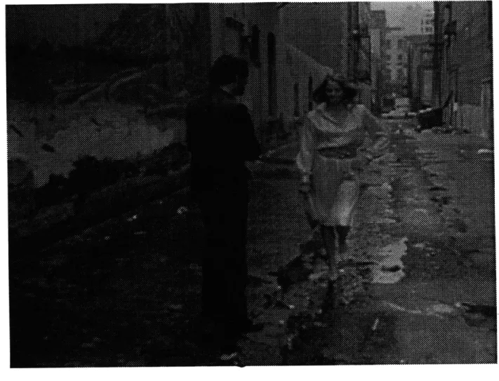
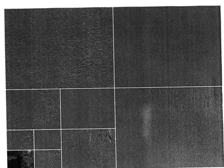
Figure2.8 is the original picture (frame 6 of second 4 of alley sequence ). and Figure2.9 illustrates the image characteristics of subbands in three level pyramid. The

j

top left, left .second from top, and the left third from top are HL bands corresponding to pyramid level 1, 2, 3, which contain the horizontal edges of the original image and some texture. The right one, two, three from bottom are LH bands corresponding to pyramid level 1, 2, 3, which contain the vertical edges of the original image and some texture. The one on the left corner is the LL band of pyramid level 3, which contains the basic shape of the original image, but blurred. The rest three subbands are HH bands from pyramid level 1, 2, 3, which contains the diagonal edges and some texture of the original image. All of the subbands here are spatial ones and no temporal

ones are shown here. From this image pattern separation, the irrelevancy reduction is obtained.

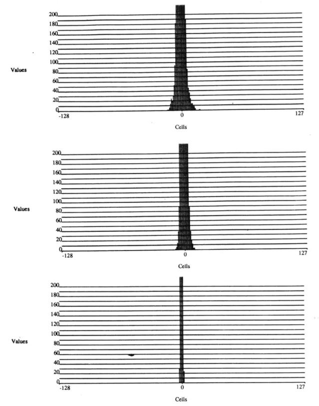
Figure2.10 contains three histograms from original picture (from frame 6 of second 4 of alley sequence), LL band of pyramid level 1, and LL band of pyramid level 3, respectively. It is easy to see that all of these three histograms have almost the same shape. It proves that the LL band in each pyramid level has the same distribution characteristic as the original image, that is relatively flat. The three histogram in Figure2.11 are from LH, HL, and HH bands of the first level pyramid, and in which the frequency value higher than 200 has been omitted. We can easily see that the variance

in these three bands is much reduced, especially, in the HH bands. Redundancy reduction has been achieved since the data with the same statistical characteristics

Figure 2.8: The original picture from frame 6 of second 4 of alley sequence.

Figure 2.9: Pyramid decomposition of the original picture in Figure 2.8.

has been localized into the same subband.

The subband analysis yields a desirable separation of the data. However, it does not provide any data compression. The data compression can be realized by non-linear quantization of subband data. This will be discussed in next section.

2.2

Vector Quantization

The technique of subband analysis/synthesis dealt with in previous section offers us subbands with desired energy distribution and visual characterization. However, a proper quantizer is still needed to reach our goal: data compression. Vector Quanti-zation(VQ) is a relatively new coding technique, but has many attractive features in image data applications, such as high compression ratios and very low decoding cost. Therefore, it has been widely used as the quantizer for the subband coding at low bit rate image communication.

5411 4876 43 379 .3 2709 Values 2167 108 541 0 127 255 Cells 1328 119 106 929 79 Values 531 39 26 1325 0 12725 Cells 69 2 5 43 Values 2 17 0 17 255 Cells

200 180 1601 140 100 60' 40 Cells Values -128 0 Cells 200 180 140 170 100 -128 0 127 Cells

Figure 2.11: Histogram for LH, HL, and HH bands of pyramid level one. Values

Now

2.2.1

_{An Overview on VQ}

Although VQ had been applied to speech already in the 1950's by Dudley [9], the use of VQ was stimulated mainly by the work of Buzo and Linde et al. in 1980 [26], who proposed a practical method for vector quantizer design based on learning, using a training set. Gray [16] discusses a large number of variations that are possible on the basic vector quantization scheme.

A quantizer is defined to be a system that maps a domain to a range in a many to one fashion. In terms of coordinate systems, a quantizer divides the domain space into regions and maps all points residing in each to a single representative value. In general cases, the term quantizer refers to the type of operation described above applied in one dimension (known as a scalar quantizer). Vector Quantization, also known as block quantization or pattern-matching quantization, is a direct extension from one-dimensional (or scalar) quantization to the quantization of multi-one-dimensional signals.

The basic VQ block diagram is shown in Figure2.12. The input X to the encoder is a vector of dimension k. In image coding application, X is a block of pixels from an image. The image is partitioned into contiguous, nonoverlapping, blocks. We chose square blocks for convenience, although nonrectangular blocks have been found

i

Figure 2.12: Vector quantization

to give slightly better performance. The encoder computes the distortion d(X, Y,) between the input X and each code vector Y, i = 1, 2,.. .,N from a codebook C. The

optimum encoding rule [26] is the nearest neighbor rule 2.6,

Y +-> d(x, yi) < d(x, yj),

j=

in which the index I is transmitted to the decoder if code vector Y yields the least distortion. We need log2 N bits to transmit the index if fixed length codewords are

employed. The quantity R = (1/k)log2 N is the rate of the coder in bits per pixel

(bpp). The decoder simply looks up the Ith code vector Y from a copy of the codebook

C, and the output X is is Y1. The performance of VQ is measured by the average

distortion D = E[d(X, X)], where the expectation is taken over the k-dimensional

An optimal vector quantizer is one which employs a codebook C* that yields the least average distortion D* among all possible codebooks. The design algorithm of an optimal codebook is not known in general. However, a clustering algorithm, referred to here as the LBG algorithm, is described in [26] which leads to a locally optimal codebook. LBG operates in the following manner. An initial guess for a representative (codebook) is made. The Euclidean distance between each input vector and each representative is calculated and the input vector is assigned to the representative that is nearest to it. After all input vectors are assigned to representatives, the aggregate error introduced by coding each input vector with the current codebook is calculated. Each vector in the codebook is then replaced by the centroid of the cluster of vectors that map to it and the procedure is repeated. The iteration will stop when the distortion reaches a minimum. However, it is impossible to bound the convergence time or to guarantee that the algorithm will converge at all. It is obvious that LBG is difficult to implement in real time.

2.2.2 - Tree Based VQ Codebook Design

Kd-tree (K dimensional tree), introduced by Friedman and Bentley [11], makes it possible to characterize multi-dimensional data as a binary search tree at the expense

of some constraints placed on the subdivision process. The application of kd-tree data structure in vector quantization is discussed in detail by Equitz [10]. In a normal binary tree, only a single binary decision may be made at any node. The kd-tree extends this in such a way that the dimension which is subdivided at each node may be different, even though there is still only one dimension chosen each time. This mechanism provides more freedom in codebook design, because a different splitting dimension may be chosen at each node according to different distortion specifications. (This will be discussed more in section 2.2.4). Since only local scalar partitions are used in kd-tree, the calculations are limited to only that node. This makes kd-tree based VQ codebook design much faster in comparison with LBG algorithm. and gives more potential for real time implementation.

Based on the above idea, Romano [22] put together the previous work done at Media Lab, MIT in his Master thesis to describe a tree structure based codebook de-sign, which partition the whole vector space into a set of unequally divided subspaces. Each of the subspaces has its local representative (code vector), the one which gives the smallest distortion among the vectors in the subspace. All of the representatives form the codebook and the elements of the codebook are linked by a k-dimensional tree data structure. Figure 2.13 depicts an arbitrary kd-tree with K = 2. The basic consideration for the design of the kd-tree based codebook are: on which dimension

i

Figure 2.13: Kd-Tree: A typical kd-tree (K = 2) shown as both a binary tree (left) and a subdivided 2 dimension space (right)

we split the. space; where on the selected dimension we split; and when we stop the subdivision.

The following control parameters are used in Romano's work

.0 Node/Dimension Selection: This parameter dictates how leaves are priori-tized for subdivision. Candidates for this include selecting the leaf (and dimen-sion within that leaf) based on the variance, cell extent, mean squared error (with respect to the representative), maximum error (with respect to the rep-resentative) or maximum number of constituents. With each iteration the leaf with the highest selection value becomes the candidate for subdivision. Note that this value is calculated for each dimension in the cell and the highest one is retained as the nodes actual selection value. The dimension that resulted in this maximum score is set to be the split axis should the leaf be selected for subdivision.

* Split Point Selection: This parameter determines how the split point along the chosen split axis is calculated. Candidates for this are the mean, median, mode or midpoint of the split dimension.

* Representative Calculation: This parameter describes the method used in

calculating the representative vector for a given cell. Candidate for this is the centroid of the cell's population in current work.

e Bounding Condition: This parameter sets the criterion which must be met before the subdivision process terminates. Candidates for this are the code book size, total distortion incurred by quantizing and Peak distortion incurred by quantizing. Note that the term "distortion" here can be replaced with any metric desired.

Even though there are 5 choices in dimension selection and 3 ways in split point selection, Romano did not explicitly explain how the combination of these parameters (up to 15 combinations) affect the output of the vector quantizer, or reconstructed images in his work [22].

Also, it should be noted that the three methods for split point selection: mean, median, middle, are identical in subband image coding practice, because all of the subbands except the lowest one have a histogram with Laplacian like distribution.

Some experiments are conducted in section 2.2.4 to examine how these parameters works.

the subdivisions. This shows a better cooperation with different distribution among subbands. However, the bounding condition here did not couple with any bit rate control. Since we are working on very low bit rate image coding, the bit allocation among the subbands becomes critical. We need to introduce a new bounding condition which can take the bit rate at each subdivision as the termination decision. This will make the explicit bit allocation in the tree based quantizer realizable.

2.2.3

Bit Rate Control in Tree Based Codebook Design

In Figure 2.12, the only information to be transmitted is the codebook index I, or codeword, if a global codebook is pre-stored in the decoder. However, some recent papers [2] [15] [17] [5] [22] suggest the advantages of codebooks which are tuned specifically for individual images or specific temporal neighborhoods. In other words, the codebooks must be incrementally updated to make the VQ useful for the low bit rate coding of images.

As shown in Figure 2.11, the peaky distribution characteristics of all of the sub-bands except the lowest one gives low entropy. In the review of noiseless source coding theory in chapter one, we know the entropy of the source data provides us a low bound

for encoding. Therefore, an entropy coding scheme should be considered in coding the vector index. As a matter of fact, this is one of the advantage of subband coding we should thereafter take.

Many practical algorithms exist that allow one to get close to, or even fall below, the theoretical limit such as Huffman coding, run length encoding and arithmetic coding [35] [36] [31]. The reason it is possible to out perform this lower bound is that some entropy coders exploit the joint statistics between samples of a signal. The entropy calculation described in Equation 2.7 only utilizes first order statistics.

Entropy, here in this thesis, is calculated from following equation:

N-1

Entropy =1 -p (xi) log2 p (xi) (2.7)

i=0

where p (xi) is the probability of the sample value x;. (This is N

=

The total number of bits used for transmission of the coded the images is given:

Our goal here is to use this total bits to terminate the subdivision process in kd-tree based codebook design. We first find out how to calculate the bits used for codebook and codeword respectively, and then apply it to the kd-tree subdivision termination.

Let us use M to denote the number of pixels in the image to be coded, and L to denote the vector dimension. Hence the total bits for codeword is:

BitScodeword = (M + L) x entropy (2.9)

In kd-tree case, p(x;) in 2.7 may be expressed as:

p(x;) number of vectors in the ith sub - space (leaf)

Total number of vectors in the whole vector space (2.10)

And N in 2.7 represents the number of subspace up to the current subdivision.

The total bits used for codebook..may by calculated as:

BitscoseNook = L x N x entropy . (2.11)

However, the entropy of the codebook is not as easily calculated as that of the code-word at each subdivision. In practice, the total bit rate of the codebook may be

calculated in either of the following two ways which approximate the bit rate by entropy calculation:

L

Bitscodebook = ceiling [log2(max[i] + min[i] + 1)] x N

Bitscodeok = ceiling log2

[n

+

(2.12)

(2.13)

A test is conducted here to see the difference of bit rate calculation of codebook among the ways represented in 2.11,2.12, and 2.13.

Table 2.1 shows the kd-tree parameter's combination used in the tests, which is also referred throughout the rest of the chapter.

Table 2.2 illustrates the test result. The test picture is the one in Figure 2.15. All of the test are terminated by error limitation at SNReak = 42db, and the total bits

used for codeword calculated by equation 2.9.

Test # Select Split

I Peak Error Mean

2 Peak Error Median

3 Peak Error Middle

4 Extent Mean 5 Extent Median 6 Extent Middle 7 MSE Mean 8 MSE Median 9 MSE Middle

10 MAX MSE Mean

11 MAX MSE Median

12 MAX MSE Middle

Table 2.1: Kd-tree Parameter's Combination

Test # Entropy Bit-added Bit-multi Error-added Error-multi

1 135398 154332 145758 0.1398 0.0765 2 118077 135468 127942 0.1473 0.0835 3 175474 200988 189822 0.1454 0.0821 4 142197 162252 153238 0.141 0.0776 5 128447 147168 138992 0.1457 0.0821 6 177597 203544 192236 0.1461 0.0824 7 210671 241740 228310 0.1475 0.0837 8 201333 231696 218824 0.1508 0.0869 9 244546 281952 266288 0.153 0.0889 10 193548 221796 209474 0.1459 0.0823 11 179678 205920 194480 0.1461 0.0824 12 216988 249336 235484 0.1491 0.0852

the second, third, and fourth column represent the total bits in which the bits for the codebook part are calculated in the ways shown in formula 2.11, formula 2.12, and formula 2.13 respectively. The fifth and sixth column shows the difference between the ways: formula 2.11 and formula2.12; formula 2.11 and formula 2.13. At the most, formula 2.12 requires about 15 percent more bits in total then formula 2.11 does, while formula 2.13 requires only about 8 percent comparatively. It is obvious that formula 2.13 offers a better approximation towards formula 2.11. Thereafter, formula 2.13 is employed in the thesis work.

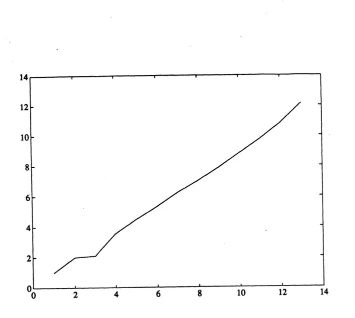
So far we have cleared the total bit calculation in kd-tree based VQ codebook design. However, there is still one assumption we need to prove before we can go ahead to apply this bits calculation method to control the termination in kd-tree subdivision. The entropy in formula 2.7 has to be monotonically increasing while N increases. To prove it mathematically is beyond the scope of the thesis. A test was run to show this assumption is generally true. The data from the picture in 2.15 is used to run the test. The X axis in Figure 2.14 represents the N in formula 2.7 in log2

scale, while Y axis shows the entropy correspondently. It seems true that entropy increases monotonically with N increasing.

14 12- 10- 8- 6- 4- 2-0 2 4 6 8 10 12 14

Figure 2.14: Entropy increasing monttonically with N in equation 2.7 increasing. The X axis represents N and Y axis represents entropy.

-current subdivision in kd-tree data structure. This provide us a possibility to realize the bit allocation scheme which is going to be discussed in Chapter 4.

The total bit rate controlled kd-tree works in a very simple iteration. The tree initially begins as a single node whose constituency is the entire vector space. The selection value, split point and representative vector are also calculated. The following loop is then executed until pre-set total bit rate is met:

1. Find the leaf with the maximum selection value.

2. Make the leaf a node and create two new leaves.

3. Calculate the selection value/dimension, split point and representative vector for both new children.

4. Calculate the total bit rate according to formula 2.8, formula 2.11, and formula 2.13.

2.2.4

Parameters in Tree Based Codebook Design

In kd-tree structure, the dimension and the point selected to do each iterative splitting are very important factors of the vector quantizer performance. A set of 12 test with different combinations of dimension selection and splitting point (Table 2.1) were run to evaluate how these combinations cooperate with total bit rate and image statistics.

Table 2.4 and Table 2.3 illustrate the experimental results from different kd-tree parameters selection combination using test picture 2.15 and 2.8 respectively. The tests use the entropy of the codeword to terminate the iterative kd-tree splitting and the entropy used here is 10.9 which is calculated by reconstructing the picture with

SNRpak = 42 db. The numbers in the first column are the tests with the kd-tree

parameters combination listed in Table 2.1. Column two gives the codebook size. Column three shows the signal to noise ratio between the original picture and the reconstructed one. Column four and five describe the total bits used by codebook and codeword respectively. Numbers in the last column are the maximum pixel value in the error picture, which is the difference between the original picture and the reconstructed one. Carefully examining the two extreme cases, the test 1 and test 8, we can easily draw some conclusions. First, test 1 uses the codebook size much smaller than the test 8, even though both of them turned out reconstructed pictures

Test # Codebook Size SNR Codebook Bits Codeword Bits Max MSE 1 3595 42.67 105080 207376 5 2 3835 41.12 111522 207362 8 3 4799 44.46 163562 207360 4 4 3971 43.25 161443 207360 8 5 4182 43.91 165556 207365 10 6 4848 44.57 177623 207364 5 7 5698 44.67 181840 207653 14 8 6117 43.71 139923 207379 24 9 6257 45.37 115795 207361 12 10 5193 44.41 121880 207363 1 1 11 5620 43.21 141366 207362 16 12 5553 45.08 165458 207361 8 13 5702 44.67 177945 207362 14 14 6105 43.71 181630 207371 24 15 6264 45.42 151038 207487 12

Table 2.3: Kd-tree Parameters Selection Tests for Picture 2.8

Test # Codebook Size SNR Codebook Bits Codeword Bits Max Error

1 4287 39.12 135398 209280 60 2 3763 36.57 118077 209281 62 3 5583 40.86 175474 209757 60 4 4507 39.05 142197 209317 60 5 4088 37.27 128447 209303 63 6 5654 40.93 177597 209438 60 7 6715 41.09 210671 209287 58 8 6436 39.27,. 201333 209284 68 9 7832 41.88 244546 209288 58 10 6161 40.88 193548 209299 60 11 5720 38.89 179678 209283 64 12 6926 41.71 216988 209284 58 13 6716 41.09 210697 209282 64

with almost. same SNR value. Second, the maxmum pixel value in the error image of test 1 is smaller than that in the error image of test 8. Here a question is raised: what does the test 8 spend more code vectors for? To find the answer, it should be recalled that a variable-rate system is used here, and, the reproduction vectors are assumed to be coded into binary strings of varying lengths according to their entropy. Thereafter, the third conclusion is that test 8 devotes more bits to the areas of discontinuity and fewer bits to areas of slowly varying intensity, while test 1 uses more bits for the slowly varying intensity such as background. In other words, test 8 favors infrequent vectors while test 1 favors frequent vectors.

One application of the above conclusions may be the consideration of right pa-rameters selection for the different subband with different energy distribution. For example, the parameters combination of test 1 may be good for the lowest subband because it has a relatively flat intensity distribution, while the parameters combina-tion of test 8 may be preferred for the higher subband which usually has a peaky energy distribution.

Figure 2.15 to Figure 2.21 are the pictures supporting the above conclusion. Figure 2.16 and Figure 2.17 have the same SNR, but Figure 2.17 used much more code vectors to code. Figure 2.18 and Figure 2.19 show that the parameters combination of test 1 in

jill

Table 2.1 perform better for the subband with a relatively flat intensity distribution, while the parameters combination of test 8 in Table 2.1 are more suitable for the subband with a peaky intensity distribution. Figure 2.20 and Figure 2.21 back up the same conclusion as the last pair of pictures do, but the image from LH subband of first level pyramid is used instead of LL band in the previous two.

Figure 2.15: The Original Picture of Flower Garden

Figure 2.16: The picture shows the error pixels of the reconstructed image from test 1 in Table 2.4. (The error image has been gainbiased by 10.) Error pixels are easily seen to concentrate in detailed regions.

Figure 2.17: The picture shows the error pixels of the reconstructed image from test 8 in Table 2.4. (The error image has been garnbiased by 10.) Error pixels appear more in the slowly varying intensity areas, like the trunk of the tree and the sky. Meanwhile, there are more peaky error pixels than that in 2.16. However, there are less error pixels in the area of flowers.

Figure 2.18: The picture shows the error pixels of the reconstructed image of lowest subband of the first level pyramid of the image 2.8. The parameters combination in test 1 of Table 2.1 is used with the codebook size = 3600. It shows much less error than next picture 2.19 which has the same codebook size but using the parameters combination in test 8 of Table 2.1. This proves that the parameters combination of test 1 is good for the subband with relatively flat intensity distribution.

Figure 2.19: The picture shows the error pixels of the reconstructed image of lowest subband of the first level pyramid of the image 2.8. The parameters combination in test 8 of Table 2.1 is used with the codebook size = 3600. It shows much more error than previous picture 2.18 which has the same codebook size but using the parameters combination in test 1 of Table 2.1. This proves that the parameters combination of test 8 is not good for the subband with relatively flat intensity distribution.

Figure 2.20: The picture shows the error pixels of the reconstructed image of LH subband of the first level pyramid of the image 2.15. The parameters combination in test 1 of Table 2.1 is used with the codebook size = 1450. It shows much more obvious errors than next picture 2.21 which has the same codebook size but using the param-eters combination in test 8 of Table 2.1. This proves that the paramparam-eters combination of test 1 is not good for the subband with very peaky intensity distribution.