Modeling ice growth on Canadian lakes using artificial neural networks.

Cllck Here

lq

Full

Article

WATER RESOURCES RESEARCH, YOL. 42, wl1407, doi:10.1029/2005WR004622. 2006

Modeling ice growth on Canadian lakes using artilicial neural

networks

o. Seidou,r T. B. M. J, Ouarda,r L. Bilodeau,2 M. Hessami.t A. St-Hilaire.r and

P. Bruneau2

Received 5 October 2005: revised 30 May 2006; accepted 7 July 2006; published l4 November 2006.

lrl This paper presents artiticial neural network (ANN) models designed to predict ice in Canadian lakes and reservoirs during the early winter ice thickness growth

period. The rnodels fit ice thickness measurements at one or more monitored lakes and

predict ice thickness during the growth period either at the same locations for dates

without measurements (local ANN models) or at any site in the region (regional ANN

model), provided that the required meteorological input variables are available. The input

variables were selected after preliminary assessments and were adapted from time series

of daily mean air telnperature, rainfall, cloud cover, solar radiation, and average snow

depth. The results of the ANN models compared well with those of the deterministic

physics-driven Canadian Lake Ice Model (CLIMO) in terms of root-mean-square error and

in terms of relative root-mean-square errors. The ANN models predictions were also

marginally more precise than a revised version of Stefan's law (RSL), presented herein.

They reproduced some intrawinter and interannual growth rate fluctuations that were not accounted for by RSL. The performance of the models results in good part from a

careful choice of input variables, inspired from the work on deterministic models such as

CLIMO. ANN models of ice thickness show good potential for the use in contexts

where ad hoc adjustments are desirable because of the limited availability of

measurements and where poor data nature, availability, and quality precludes using

deterministic physics-driven models.

Citation: Seidou, O., T. B. M. J. Ouarda, L. Bilodeau, M. Hesstrmi, A. St-Hilaire, and P. Bruneau (2006), Modeling ice growth on Canadian lakes using artificial neural networks, lYater Resour. Res.,42, Wll407, doi:10.1029/2005WR004622.

1. Introduction

[z] This paper investigates the capacity of artificial neural networks to simulate the growth of ice thickness on Canadian lakes. Although the growth of ice thickness can be modeled with nurnerical physically driven models, the lack of suffrcient and precise data is often a linritation to the applicability of this kind of models. On the other hand, extensive records of meteorological variables such as temperature, rainfall and snow on the ground are widely available over the Canadian territory, along with ice thickness measurements on a number of lakes. Neural network models are often proposed for situations where the physics of the involved processes may be cornplex or not fully defined, and where an extensive data sct is available for training a network while being incomplete from the point of view of deterministic physically driven models [e.g., Olsson et a1,, 2001; Cannon and Whitfield, 2002; Hewett,2003l.

[l] Several artificial neural network (ANN) models of lake ice thickness growth are considered in this study. One of these ANN models is regional in scope and is applicable

rCentre

Eau,'['ene et Ënvironnement, Institut National de la Recherche Scientifi que. Quebec, Quebec, Canada.

rHydro-Québec,

Montreal, Quebec, Canada. Copyrighl 2006 by the American Geophysical Union. 0043 - | 397 i 06 t2005WRO04622$09. 00

to any location in the country, while the others are specific fo the measurement station to which they were adjusted. The results of the ANN models are compared to those of a modified version of Stelàn's law and to published results of the detern.rinistic model CLIMO (Canadian Lake lce Model) lMenard et a\.,200?a.2002b; Dugualt et aL.,20031.

[+] The remainder of this paper is composed of six parts: an overview of ice growth rnodels based on thermodynamic principles (section 2), an introduction to artificial neural networks (section 3), the methodology for choosing input variables and rating results (section 4), the case study ofice growth on Canadian lakes (section 5), resr.rlts and discussion (section 6), and finally, conclusions (section 7).

2. Ice Growth Models Based on Thermodynamic Principles

[s] This section presents an overview of ice growth models based on thermodynamic principles. Special atten-tion is given to the formula known as Stefan's law, and to a modified formr.rla referred herein as the revised Stefan's law (RSL), as this formula is later used with the same data sets as the ANNs in order to compare their performances in predicting ice thickness.

[o] Formation and evolution of river and lake ice are govemed by heat fluxes in the water body, heat transfers at the interfaces of air-watcr, air-ice, water-bed, and water-ice, and by radiation exchanges with ahnosphere. The different

wI1407

components of the energy budget are not easy to quantifu since they are related to hydraulic conditions (turbulence and velocity distribution), turbidity (which has an effect on the absorption ofradiation energy), the albedo and the depth and compactness of snow above the ice cover.

[r] All numerical ice growth rnodels use a more or less simplified version of energy budget. Some of these models apply to a specific aspect of ice development such as the ice cover initiation lSchulyakovskii, 19661, border ice formation fMatousek,1984; Svensson et a\.,19891, frazil ice formation fomstedt, 1985a, 1985b; Svensson and Omstedt, i9941, and ice cover growth [e.g., B eltaos, 199 5; Schulyaknvskii, 1966; Lock, 19901. Other models are more complete and may sirnulate ice fonnation, transport, growth and decay lShen and Chiang,1984; Shen and Ho, 1986; Shen et al.,1990,

1e951.

[t] They all use energy balance to compute ice evolution. They differ from each other by the level of details used to describe ttre different aspects of the phenorncnon: hydrau-lics, heat transfer and radiation. Lake ice models are sirnpler since water velocity is low enough to justify the use of one-dimensional energy balance models [e.g., Stefan and Fang, 1997; Fang et al.,1996; Dugual, et aL.,20031. For Canadian Iakes, Ménard et al.12002a,2002b1 used a one-dimensional thermodynamic lake ice model called CLIMO (Canadian Lake lce Model) which computes vertical water temperature profiles by solving the heat equation taking account ofsolar radiation penetrating the water body, ice cover and snow on ice. CLIMO is a modified version of a one-dimensional sea ice model [Flato and Brov,tr,1996] and has been described in detail by Duguay et al. 120031. The inputs of the model are daily mean temperatures, wind speed. reiative humidity, cloud cover, snow depth on the ice and lake latitude. Outputs are dates offreeze/thaw and ice thickness. Mënard et al. l2002al used CLIMO to simulate ice growth at station YZF (Back Bay) for the years 1960-1991, and ir repro-dr.rced ice thickness with a mean quadratic error of 9 cm. They also simulated ice thickness for the years 1977 -1990 at station YFL (Fort Reliance) and obtained a root-mean-square elror of l8 crn.

[e] Another themrodynamic lake ice model was pre-sented by Fang et al. |9961 to compute ice thickness and dates of freezelthaw on lakes located in Minnesota, USA. The model solves the heat eqr-ration along a vertical axis and uses wind-triggered surface layer mixing and water temper-ature as criteria for predicting the ice cover formation date. Tlre mean quadratic error for ice thickness predictions was 2 cm (for a maximal observed thickness of 55 cm) when this model was validated on lake Ryan located in Minnesota, USA.

[to] This kind of model requires types of data that are not always available, unless there is a meteorological station close to the site. Consequently, in practice, simplified formulas are used based on air terrperature.

[rr] The simplest and the most widely used formula is the Stefan's law (SL) which could be derived by simpli-fying the equations obtained using energy balance [e.g., Lock, 19901:

t u : k J D , t

( l )

where 1{ is the ice thickness, Da is the sum of degree-days below the freezing point since the onset of the ice

SEIDOU ET AL.: ICE GROWTH ON CANADIAN LAKES w t t 4 0 7

cover in any given year, and fr is a constant. In practice É is used as an adjustable parameter with a value that is lower than the theoretical value to account lbr varying conditions of exposure and insulation; Michel ll97ll gives a range of values adapted for a variety of lakes and rivers.

[rz] The date of the onset of the ice cover is a basic parameter for using Stefan's law as it determines the date at which the accumulation of freezing degree-days is started for any given winter. For the majority of sites of interest in this study, this date is not known so that the normal usage of Stefan's law was not feasible. lt was therefore decided to use a "revised Stefan's taw" (RSL), which is based on Dn, the accumulation of freezing degree-days starting with the first day of below freezing air temperature in any given season. RSL presents one more adjustable parameter, C, the eflèctive number of degree-days to be subhacted from Dn in order to obtain D.1.

" , _ [ r J D * T , " f D r 2 C t ) \ l 0 { D r < C V r The parameter C will normally take on a positive value since the date of ice onset arrives several days or weeks after the occun'ence of the first day of freezing daily mean alr temperâture.

3. Artificial Neural Networks

[t:] An artificiai neural network (ANN) is a set of simple cornputational units or processing nodes grouped in layers and working in paraliel. It is ca11ed a neural network because the processing nodes mimic the behavior of biologic neurons. These nodes are also called neurons. In the nctwork, each layer makes an independent process-ing of the information and forward the results to the next layer. The information given to the network passes frorn the input layer to the output layer through optional intermediate layers (or hidden layers). An ANN model can have more than one hidden layer. However, research has shown that a single hidden layer is sufficient for ANNs to approximate any complex nonlinear function fCybenko, 1989; Hornik et al., 1989). A larger number of hidden layers can speed up the learning process, but many experimental results seem to confirm that one hidden layer is su{ficient for prediction and forecasting problems fZhang et al., 1994; Coulibafu and Anctil, 1999; Coulibaly et aL.,20001. Artificial neural networks have the ability to memorize empirical knowledge and make it available for use. The empirical knowledge relbrs here to the unknown relationship between observed data series. This ernpirical knowledge is acquired through the learning algorithm, which essentially modifies intemal tleuron parameters to fit the outputs of the neural network to the observed response variable. The acquired knowledge is mernorized in the synaptic weights, obtained by a training or adaptation process. Finally, this knowledge is restituted when the model is used to simulate the response variable on new input data sets. The use of ANNs is deemed to be particularly useful when the physical processes are com-plex and not fulty detined, when the model has many uncertainties (model coefficients andior input parameters), and when there is extensive data for trainins the network. 2 o f 1 5

w n 4 0 7 SEIDOU ET AL,: ICE GROWTH ON CANADIAN LAKES

LINEAR NEI}RON

\ry11407 rons in the hidden layer and a linear neuron iu the output layer lHagan, 19961:

antt : J:n+t (ilr^+t a^ + B'*t) m = 0, | (3) where, a0 is ttre network input, al is the output of the hidden layer, az is the network ouçut, /t and f2'are respectively sigmoid and linear transfer functions:

Figure l. Architecture of a tèed forward network with two neurons at the hidden layer and one neuron at the output layer.

It is a "black box" type of model for which the user has no control on the intemal behavior, and it can poorly perform when used for generalization especially when the number of neurons is too high for the complexity of the problem (overfitting). In hydrology, ANNs have been used for hydrologic data classification [e.g., Liang and Hsu, 19941, _{river discharge prediction le.g., Sham,seltlin,} 19911, evaluation and forecasting of \vater quality [e.g., Zhang et al., 1994], inflow forecasting for irrigation and hydroelec-tric darns le.g., Coulibaly et al., 20001, rainfall estimation [e.g., Xiao and Chantlrttsekar, 1997], and correction of streamflow under ice lOuarda et a1.,2003).

4. Methodology

[ta] The capabilities of RSL and ANNs to model ice growth on individual Canadian lakes are investigated. The performances of the ANN models are investigated as function of its input variables and their intemal structure, and a procedure is set up to select the best perfomting models.

[ts] Two kinds of ANN models were considered in this stndy: (l) site specific ANN models were trained and validated with ice thickness data from a single site and (2) a regional ANN model was also constructed in order to simulate ice growth for sites without field measurements of ice thickness. Each model is characterized by the set of its input variables (referred to as a combination of input variables), and the ANN architecnrre (defined by the num-ber of neurons on the hidden layer).

[te] Choosing the best set of input variables and assess-ing the performance of a model requires some performance criteria, some model validation procedures, and a method of picking the best model among all possible configurations. Since our models are data-driven, two validation procedures were used to ensure that the final ANN rnodels are properly hained and can be used with confidence for generalization purposes. These validation procedures are described at section 4.4.

4.1. Architecture of the Artilicial Neural Networks [n] The artificial neural network used in this resealch was a one-hidden-layer neural network with sigmoid

neu-.f'(r):#,

f , ( n ) : , ,

L/'"*t and, B'''L are network weights and biases

defined with the following formulas:

HIDOEN LAYÊR OUPW LAYER

(4) (5) which are

| 4'T'

w ^ r t : | , .

L

"t_:1.,

m : 0 , 1

where ,56 is the nr.rmber of input variables, Sr is the number of neurons at the first layer and 52 is the number of neurons at the second layer.

[ta] One-hiddenJayer neural nefworks with sigmoid ac-tivation function on the hidden layer and a linear acac-tivation neuron were shown to be able to approximate any bounded continuous function with arbitrarily small enor fCybenkn, 1989], provided the number ofneurons in the hidden layer is sufficient. Because of the neurons with sigmoid activation functions in the hidden layer, this ANN model is not a linear nrodel. Other architectures may have been chosen, br.rt there are no rules for choosing the number and the sizes of an ANN model. For instance, it is believed that increasing the number of layers can increase the learning capabilities of the model, but it also increases the number of parameters and thus the length ofthe series required to properly train it. For the onset of this study, the simpler and most popular architecture was chosen.

[rs] Figure I shows the architecture of a one-hidden-layer neural network with three input variables, two neurons in the hidden layer and one neuron in the output layer. The synaptic weights are obtained using a supervised training algorithm using Bayesian regulation lMackay, 1992, 199 51. In supervised training, both the inputs and the outputs are provided. The network then processes the inputs and compares its resulting outputs with the desired outputs. Emors are then propagated back through the system, cansing the system to adjust the weights which control the nefwork. [zo] An iterative trial and error process, described in more details in the rest of the paper, will be used to set tlre optimal number and nature of input variables as well as the number of neurons in the hidden layer.

4.2. Selection of lnput and Output Variables

[zr] ANNs are data-ddven models, so their performance for a given problem relies on the relevance of the inpuV output variables that are considered in the training process, and on the complexity of the relationship between inputs

/iij I

[àî*''l

,(-,-lrr.l

' 8""

:

_lru,;]

tu'

w11407 SEIDOU ET AL.: ICE GROWTH ON CANADIAN LAKES

Table l. Tested Combinations of Meteoroloqical Variables w l l 4 0 7 and outputs. As it is the case for physically driven models,

problem pararfieterization can dramatically change algo-rithm efficiency. The purpose of the ANN being the prediction of ice thickness, the formulation of its input and output variables was guided by these practicai consid-erations: (l) inputs should be rneaningful for the ice growth process and available at all ice measurement stations, (2) the sensitivity ofthe output variable to input variations should be as high as possible to enhance training efficiency, and (3) the sensitivity of the output variable to input variations should have the sane order of magnitude for all input variables.

4.2.1. Output Variable

lzzl At first, it seerned obvious hhat Hl the ice thickness, should serve as tlre output of the ANN. Early runs of the ANN showed however that the ANN relied almost exclu-sively on the sum of freezing degree-days and made little use ofthe other variables (presented below). The reason for this is that the influence ofthe sun offreezing degree-days on the output function was so strong that the training algorithm (which is basically a numerical optimization algorithm) was unabie to account for the effect of the otirer variables. Other variables closely related to the ice thickness were then sought with the intent of improving the fit between observations and predictions of ice tlrickness.

[z:] After some exploration, the output variable that was retained for this study is the parameter HilDl, which corresponds to the Stefan coefficient. Once a time serics ofthe growth rate ofthe square ofthe ice thickness has been computed, a time series of ice thickness is easily recon-structed. The parameter HjlDl is drawn directly from the classic Stefan's law and represents an instantaneous evalu-ation of the square of its constant Ë. Using this output variable led to a reduction of the weight of the degree-days input variable in the ANNs, compared to that of other input variables, and presnmably allowed the ANN to extract additional information from the other input variables. It was found that this choice of an output variable increased appreciably the precision ofthe ice thickness prediction and led to a better comprehension of the eftèct of the other variables in rrodeling the ice thickness.

4.2.2. Input Variables

[z+] In the present shrdy, selecting the input variables of the ANNs was a two step process. First, candidate physi-cally observed variables were identified. Then, ANN input variables were formulated using the physically observed variables. These physically observed variables were retained according to their availability and recognized significance for the heat budget involved in ice growth: (1) daily mean air temperatrre, (2) daily total solar radia-tion, (3) daily rainfall, and (4) daily snow depth on the ground (as measured at weâther stations). Longitude and latitude were also tested as additional parameters for the regional neural network model.

[zs] The preceding variables were used to construct a variety of variables, to be used singly or in linear combi-nations as input variables for the ANNs. When these variables are sums, the sumrnation starts on the first day of frost based on the daily mean air temperature and ends on the day assigned to the variable. The following variables were considered and computed for each winter: (1) the sum of freezing degree-days derived from the air temperature

Clombinations of

Meteorological Variables Variables' I 2 3 5 6 7 8 9 l 0 l l t 2 T J l 4 l 5 t 6 t 7 l 8 l 9 70 2 l 22 2 3 Da; Rad,,

Da; Rad,.. + 0.25 Rad,, Dd ; Rad'," + 0.50 Rad, Da; Rad,. +. 0.75 Rad" D1 ;Rad,,"+ Rad" D 6 ; R a d , . ; F g Da; Rad,,.+ 0.25 Rqd; Fls D1 ; Rad* + 0.50 Rad";I{ s Da ; Rad," + 0.75 Rad"; È g Dd; Rad^" + Rad"; H s D7; Rad^";R

Da; Rad,," + 0.25 Rad.;R Da; Rad,,. + 0.50 Rdd.;ll D,; Rad," + 0.75 Rad";R Da: Rad,," + Rodc;R Da; Rad,";H"; R Da ; Rad,. + 0.25 Rad; FI s I R Dd ; Rad^. + 0.50 Rad"; F! 3; R D d ; R a d , , . + 0 . 7 5 R a d c ; Ê 3 ; - R D6 Rgd," + r1o4;Às; F Da )_Hs DaiR D a ; H s ; R

'Note is used only for data preprocessing and posprocessing.

D"("Cdav), as was already described earlier in this paper, (2) the sum of solar radiation during the period of ice growth for days with precipitation (W daylm'), divided by the sum of degree-days ,Rad" (this quantity is a proxy to the quantity of solar radiation attemrated by cloud cover), (3) the sum of solar radiation during the period of ice growth for days without precipitation (W daylm-), divided by the sum of degree-days Radn", (4) the average daily rainfall (over time) during the ice growth period R (mm), and (5) the average on-ground snow depth (over time) during the ice growth period Hs{cm).

[zo] The sum of degree-days D, was used to compute HllD, on the calibration data set (preprocessing), and to reconstruct ice thickness time series from simulated series (postprocessing). It wiil be referred to as an input variable in the remainder of the text.

[zz] The sum of solar radiation was split into two parts because only the total amount that reaches the ground should be considered. Consequently, attenuation due to cloud cover has to be accounted for by multiplying Rad" by a positive factor * smaller than or equal to l. Five sets of combinations of Rad," and Rad. were considered: Radn., Radn,+025 Rad,, Radn. Rad., Radn"+0.75 Rad", Rad,,"+ Rad., corresponding lespectively to o : 0,0.25,0.50, 0.75 and 1. A total of 23 sets of combinations of meteorological variables (listed in Table 1) were tested as inputs for the artificial neural network models.

[zs] Other important variables for ice growth would have been variables based on lake morphology such as maxlmum depth, mean depth, surface area, perimeter length and other variables that could be derived from these. For most of the lakes considered, depth information could not be found within the scope of this study. Other parameters basecl on the surface area and lake shape ol1 maps were not used in the eird. It should be noted that this information is never-4 o f 1 5

w l l 4 0 7 SEIDOU ET AL.: tCE GROWTH ON CANADIAN LAKES w r 1 4 0 7

140 120 100 80 60 1,O 120 lm 80 Longitude (W)

Figure 2. Location of the 26 lake ice measLrrement stations.

theless considered to be relevant, particularly for the eval-uation of the date of freezeup. It is felt by the investigators that the use of morphological lake data could provide interesting avenues for the use of the ANNs ibr the modeling of lake ice in future studies. They would require a specialized focus on sources of data that could not be explored within the framework of the present study. 4.3. Performance Criteria

[zo] The performance of a given ANN model is evaluated using five performance criteria: root-mean-sqr.rare error

Table 2. Ice Thickness Measurernent Stations

(RMSE), relative root-mean-squal€ error (RRMSE), model

explained variance (l), Nash criterion (NASH), and bias

(BIAS). The criteria are defined as follows:

RMSE:

Gtr,

- uïf)'

(7)

RRMSE:

_{(;e e"!)')'}

, , -

c o v ( [ n ] . . . n ' l , l

t , . . . ,

^ ' l ) 2

.

'

v a r ( f v | , .

. . , n i l ) v a r ( i n

j ,. ,nf}"

B ' A S :

_{l i fal - rf)}

( r o )

t r - '

D@f - nf)'

N A S H : t - o i ( 1 r )

\ta'; - rt,1'

where .Hf,i : 1,..,n and nf,i : 1,...,n are observed and simulated ice thicknesses.

4.4. Validation Procedures

po] Two validation procedures were used: the leave-one-out cross-validation procedure to find the best combi-( 8 )

(e)

Station Code Station Name Water Body

Longitude, Latitude, H A 1 " L I ' I WFN' WIQ WLH" WHO WTL" YAH" YBK, YBT" YBX' Y E I " YGK" Y G M " YGV YIV" YKL' YNE YNI YPY" YQl' YVP, YYR" Y Z E YZF" YFL, 6 8 . 3 6 6 1 . 5 1 0 5 . t 5 109.93 86.09 7 3 . 6 9 8 8 . 1 1 I L . J O 95.96 1 0 0 . 3 I 5 6 . 8 I 99.09 / ) . J 9 5 . 0 1 6 3 . 8 8 9 3 . 3 1 6 5 . r 9 9 6 . 1 6 69.08 I I 0 . 8 3 8 8 . 7 8 6 7 . 5 3 5 9 . 5 8 8 l . 9 t 3 1 1 4 . 3 4 I 0 8 . 8 6 6 1 . 0 3 82.46 ) / . J J 54.76 52.21 46.03 5 3 . 8 r ) J . / O 64.3 5 7 . 8 6 5 1 . 4 5 6 1 . 1 1 44.7 5 0 . 6 1 50.29 5 3 . 8 4 5 4 . 7 8 5 3 . 9 8 5 3 . 1 8 5 8 . 7 48.43 5 8 . 1 1 5 3 . 3 3 45.54 62.45 6 2 . 7 0 Quaqtaq Alert Cree Lake Primrose Lake Lansdowns house Sainte agathe des monts Big trout Lâke La grande IV Baker Lake Brochet tslancMsablon Ennadai Lake Kingston G i n l i

Havre Saint Piene Island Lake Scheiferuille Noruay house Nitchequon l'ort chipewyan 'l'hunder bay Kuujjuaq (ioose bay South baynrouth Yellorvknife Quaqtaq Unnamed Lake Upper Dumbell Lake Cree Lake Primrose Lake Attawapiskat Lake Lac des sables Big trout Lake Lac la Tanière Baker Lake

Brochet bay of Reindeer Lake Lac à la Truite

Ennadai Lake Lake Ontario-Horsey Bay Lake Winnipeg Patterson Lake Tsland Lake Knob Lake Little Playgreen Lake Nitechequon Lake Lake Athabasca Thunder Bay Stewart Lake Tenington Basin Huron Lake (South Bay) Great Slave Lalie (Back Bay) Great Slave Lake (Fort Reliance) "Stations

with enoush data to calibrate local ANN models.

w 1 1 4 0 7 SEIDOU ET AL.: ICE GROWTH ON CANADIAN LAKES w l t 4 0 7

nation of input variables aud ANN structure, and the standard split sample procedure in which the data is split in two subsets, the first being used to hain the neural network and the latter being used to check the model performance.

[lt] The leave-one-out procedure aims to assess the generalization capability of a given ANN model. In the leave-one-out procedure, the data is divided in subsets. A subset is represented by all measuremeûts during a year (for local ANN models and RSL) or all measurements at a given site (for the regional ANN model). All subsets but one are used to train the neural network. Then the trained ANN model is used to simulate the subset that is left out. The same process is repeated so that every subset ofthe data is left out once. The performance indices are then computed using the observed and sirnulated values over the whole data set. The pair of input variables and ANN structure which best explain the data is then selected for the rest of the procedure. Unfortunately, the leave-one-out procedure does not give a final model since the neural network is trained several times (one time for eaclr subset) to compute the perflomrance indices.

pz] The objective of the split sample validation proce-dure is to have a trained neural network to use for the rest of the study. In this procedure. the data is repeatedly and randomly divided into two parts containing 80% and 20% of the observations. The first part is used to train the ANN and the other is used to rate it. The operation is performed twenty times and the pârameter set of the run which gives the srnallest RMSE is retained and completes the assembly of the rrodel.

4.5. Selection of the Best Combination of Meteorological Variables and ANN Structure

[r] First, all possible pairs composed of a set of input rneteorological variables (listed in Table l) and a network structure (defined by the number of neurons in the hidden layer) ale formed, given that the number of neurons on the hidden layer is constrained to be less than 10 for compu-tational purposes. For example, the pair (3, 7) rcpresents an ANN model with seven rleurons on the hidden layer and for which the inputs variables arc D4, Rad,,, + 0.50 Rarl.. The performance criteria of each pair are then rated using the leave-one-out procedure.

[l+] When some values of an input variable (such as surn of rain or snow on ground) are missing at a given site, the combinations of meteorological inputs containing that variable cannot be used. In this case, only a part of the 23 possible combinations of inputs ale tested when searching the best local ANN model. To avoid this situation with the regional ANN rnodel, it was trained and validated with tlie data of the measurement stations where the entire input variable were available.

psl The best pair is then chosen, and the cornbination of meteorological variables in this pair is considercd to be the one which best explains the data, while the number of neulons in the pair defines the best ANN structr-rre.

5. Case Study

5.1. Data

pol The data used in this study is of three types: (l) ice tlrickness data from the Canadian lce Service [2005],

E i;c t0: c[

f,

0 5I] 10ûr 150û 2ttû &Ê 3ù+l 35æ 4m i5m

Sum o, ljegre.Days

Figure 3. Identification of ice growth phase in the data sets at station YZF: (a) all observations and (b) ice growth phase.

(2) daily meteorological data obtained from Environment Canada, and (3) incident solar radiation at the top of atmosphere which have been computed as function of time and geographic location of the studied sites using the formulas presented in Appendix A.

pz] The data set contains ice tbickness and snow depth measurements on 53 sites located on Canadian lakes fLenormand et a1.,20021. Only 26 ofthese sites have years with enough measurements to calibrate Stefan's law and the local ANN. Eight of these stations were not used for calibration and validation of the regional ANN because of data availability issues that will be further explained. The 26 ice measurement stations are listed in Table 2, and their geographic locations are presented in Figure 2.

[:a] The weather data was provided by the national climatic archives of Environment Canada and contains the daily data of temperature, precipitation (snow and rain) and snow on the ground for more than 10,000 stations distributed all over the Canadian territory.

5.2. Proxy Variable for Solar Radiation at Ground Level

[:e] Solar radiation was considered as a relevant variable at the onset of tbis study because radiative fluxes were recognized to be a significant part of the lake energy by most authors [e.g., Lock, 1990; F'ang et a|.,1996; Menard et a1.,2002a, 2002b; Duguay et al., 2003). Howeveq solar

500 100û 150û :û0t 2gD 3u 35û)

Sum ûf0e0pe-0ays

wn407 a)

SEIDOU ET AL.: ICE GROWTH ON CANADIAN LAKES w l l 4 0 7 temperature on a given date at a given point is interpolated using the observed values at the nearby stations: a data processing program secks the nearest weather station suc-cessively in the northeast, northwest, southwest, and south-east quadrants. the temperature of the ice measurement site is computed as the weighted average of the temperatures at the weather stations. The weights are inversely proportional to the distances frorn the site of measurement to the weather stations. If historical measurements are not available at the ten closest stations in a quadrant on a given date, the data is considered missing. When a variable (such as rain, degree-days or snow) has missing values, the combinations of inputs containing this variable cannot be used. This may happen when weather stations are too far frorn the ice measurement station. In this case only part of the 23 possible combinations of input listed in Table I can be considered. At eight of the 26 lake ice thickness lneasure-ment stations, some irregularities were observed in the data (such as a long delay between first freezing air temper- 90-80. 50' 40" l w -110 124 1m 80 60 140 120 100 80 Longitudo (W)

b)

140 120 1oo 80

-'l1*"1ffi

120 1oo

Figure 4. Spatial variability of RSL

a) parameter C; b) parameter k.

BAKER LAKE YËK. CALIBRATIOI{

*- :tt iÀI

*+'*

{.*

+

2m 3m0 40m

BAKÉR I.AKË Y8K. VALIDATION

a)

300 æ0 1 ù 0

0

radiation measurements at the ground level were not avail-able in su{Iicient quantity since they are not measured at al1 weather stations. As an altemative, assumed ground level solarradiation was calculated using solar radiation on top of the atmospirere multiplied by a factor o; ci is equal to the unity on days without precipitation, and lower than the unity on days when rain or snow was observed. The values of solar radiation on top of the atrnosphere were calculated as functions of the date and the geographic location according to an algorithm giveir in Appendix A.

5.3. Spatial Interpolation of Weather Data

[.lo] As geographic positions of the ice measuring sites did not coincide with that of the weather stations. the air

*

*

+ jhFiÇF- ₊ + ObseP6d - Simulaled(revised 0 2m0 3000 40to Srm of 0egree-days 0 10ù 2ao s)l 400 5t0 6tl ?ff 80ù S u m o f D e q r e e - d a v c

Figure 5. Observed and simulated (RSL) ice thicknesses versus sum of degree-days at some ice measurement stations: (a) YBK (Baker Lake) and (b) YGK (Kingston).

250 I 3 t5o Ë too

E s u

8B 60 40 x BO E .-.. ! l N Ë 4 0 ; 2 0 0 0 80 parameters:

KINGSION YGK. CALIBRATIOI.I

KINGSTON YGK. VALIDATION

wl1407

Table 3. Performance Criteria tbr the Revised Stefan's Law

SEIDOU ET AL.: ICE GROWTH ON CANADIAN LAKES wll407

Calibration Validation

Station

k,

a'n 6-0.s oç-o.s I RRMSE

L , d ' c RMSE, cm B I A S , cnl R M S E . cm .2 _RRMSE BI,AS,_cm H A I L T I WFN WIQ VYLH woH WTL YAH YBK Y B T YBX YEI YCK Y G M YGV YIV YKL YN-E Ylit YPY YQ' YVP YYR YZE Y7F YFL Muimum Minimum Mean 1 4 . 0 6 4 6 . 1 6 90.23 2 3 1 . 5 0 33.67 60.66 14.72 6 2 . 7 3 1 5 4 . t 2 t 2 . 8 7 56.24 44.42 209.03 58.67 l 08.00 1 4 0 . 3 3 5 9 . 8 7 1 0 . 7 1 57.78 9 5 . 1 9 147.73 5 8 . 8 9 l 6 . 5 8 58.27 52.98 4 2 3 . 2 4 2 3 . 2 0 1 0 . 7 1 8 9 . 1 8 4.97 I 1 . 9 4 4 . 1 7 6 . 2 1 5 . 8 7 4.94 ),tr I 5 . 5 3 6.07 6.50 7.92 7.29 4 . 8 3 5.90 5 . t 5 5 . l 4 6 . 2 9 8 . 0 5 5 . 8 1 1 0 . 3 0 4 . t 9 6 . 2 4 7 . 8 0 5 . 7 5 6 . 5 7 1 5 . 2 4 t5.24 4 . 1 7 6 . 7 0 1 . 0 2 3 . 1 6 0 . 1 0 -2.94 - l - / o 0.73 0 . 4 9 - t . 9 9 4 . 2 7 -0.28 1 . 0 8 4.06 3 . 1 7 l - o J 1 . 2 4 0 . l5 0 . 8 3 2 . 8 8 2 . 1 7 | . 2 5 * 1 . 0 6 2 . 7 8 't.62 -0.92 2 . 2 1 - 0 . 3 0 --.2.94 0 . 9 8 9 . 8 1 30.29 14.84 8.49 9.34 8 . 4 r r 3 . 8 2 1 0 . 6 5 I 1 . 6 9 7.32 21.86 13.64 1 0 . 5 1 14.20 3 2 . 8 7 | . 2 2 l 1 . 3 8 9 . 2 6 9 . 4 1 l 3 . 8 3 lt.24 t t . 4 4 | 3 . 6 8 6.95 1 3 . 8 0 2 . 2 1 3 2 , 8 7 2 . 2 1 12.78 0.96 0.72 0.68 0.74 0 . 8 3 0 . 8 2 0.87 0 . 8 9 0.96 0.92 0.83 0.92 0.77 0.85 0 . 7 4 0.76 0 . 9 1 0 . 8 8 0 . 8 9 0 . 7 0 0 . 8 0 0.95 0.67 0.74 0 . 8 4 r 3.80 r3.80 0 . 6 7 1 . 3 2 - J . ) ô 4 7 . 3 0 -6.68 2.90 3 . 6 1 1 . 2 0 - 8 . 0 9 7.20 -4,22 - t . J ) t 9 . 1 2 2.94 8 . 3 1 , 9 . 8 1 28.97 1 . 7 8 - ô . ) _I 10.46 -5.44 8 . 6 5 5 1 . 1 0 6 . 2 8 3 . 0 5 2 . 3 0 0.27 0 . 2 7 5 1 . 1 0 - 9 . 8 1 6 . 1 6 2 . 8 0 2 . 5 7 1 . 5 4 1 . 8 4 t . 8 6 2.06 1 . 9 5 1 . 7 6 3.05 | . 6 4 2 , 9 1 2.70 2.70 2.22 2 . 5 ) 1 . 8 8 2.09 2 . t 2 1 . 7 5 1 . 8 9 3 . 1 3 2 . 5 3 2 . t 6 2 . 3 2 2 . 1 4 1 . 9 9 J . I J 1 . 5 4 2 . 2 3 0 . 9 8 0.90 0 . 8 6 0 . 8 4 0 . 7 0 0 . 6 9 0 . 9 1 0.93 0 . 9 7 0 . 8 6 0 . 7 2 0 . 8 1 0 . 7 1 0.60 0 . 8 7 0 . 6 9 0.92 0 . 8 0 0 . 9 2 0 . 5 5 0 . 7 4 0 . 8 6 0.'73 0 . 7 0 0 . 8 5 0 . 8 0 0 . 9 8 0 . 5 5 0 . 8 0 0.05 0 , 1 2 0 . 0 7 0 . t 7 0 . 1 0 0.08 0 . 0 8 0 . 1 0 0 . 0 6 0 . l l 0.23 0 . 0 8 0.40 0 . 0 7 0 . l 0 0 . 0 8 0.07 0 . 2 1 0 . 1 I 0 . 2 6 0 . 0 8 0 . 0 8 0 . 1 6 0 . l 3 0 . 0 9 0 . 0 9 0 . 4 0 0 . 0 5 0 . t z 0.09 0 . l 9 0 . l 6 0 . 2 8 0 . 1 4 0 . t 8 0 . l 5 0 . l 6 0 . l 0 0 . t 4 0.50 0 . l3 0 . 9 1 0 . 1 5 l . l 3 0 . 1 9 0 . 1 5 0 . 1 7 0 . 1 3 0 . 2 9 0.92 0 . 1 2 0 . 1 9 0 . 1 6 0 . l 6 0 . l 6 l . l 3 0.09 0 . 2 7

atures and the ice growth starting period, or nrissing values in some of the interpolated weather variables) so only the 18 remaining stations were used forthe construction ofthe ANN models. These stations are indicated in Table 2. 5.4. Elimination of the Period of Thinning at the End of the Winter in the Data Set

[ar] The model developed in the present study is appli-cable to the growth phase ofthe ice thickness. It is therefore important to eliminate the period of ice thinning which happens at the end of winter. For this purpose, we use an empirical iterative procedure: starting from the end of the data series and moving toward its beginning, all measure-ments are successively considered for eventual rernoval. All the dates when the measured ice thickness happened to be higher than the average ice thickness of the remaining subsequent rneasurements. Previously elirninated values are not accounted for when cornputing the average ice thickness of the remaining subsequent measurements. When a given measurement is removed, all subsequent ûleasure-ments are also rernoved. This practical procedure insur.es tirat the thinning period, and part of the period when the thickness stagnates are eliminated. The rcsults of the appli-cation of such a procedure to station YZF are illustrated in Figure 3. Figure 3a presents the wbole set of measurements including the thinning period and displays several step drops on the ice thickness which would have affected the training of the ANN models. The retained nleasuremenrs after application ofthe proposed procedure are illustrated in Figure 3b. These results corespond to what was expected

when designing the procedure and were used for subsequent analyses.

6, Results and Discussion

[+z] The data sets described in section 5 were used to calibrate the RSL, and to train the local and regional ANN models. ANN training and simulations were performed using the Neural Networks toolbox of Matlab fThe Mathvorks, 20051. The training function (trainbr function in the Matlab environment) uses Bayesian regulation p4ackay, 1992, 19951 to enhance generalization capabili-ties. The maximum number of epochs is set to 1000, and the minirnum gradien^t (for minimization of the objective function) to I x l0-'". The training algorithm also uses an adjustable parameter p-u which controls how far the next values of the parameters will be searched during the optimization process. lr,max was set to its default value in M a t l a b . i . e . - 1 x 1 0 ' " .

6.1. Comparison of RSL ând Local ANN Models [+:] The spatial variations of RSL parameters are illus-trated ûr Figure 4, and no trend could be found with respect to geographical location. It was found that RSL l'epresents an excellent ice growth model when it is calibrated for a given site. Observed and sinnrlated data are represented tbr sorne of the ice thickness neasurement stations in Figure 5. The pararneters of Stefan's law are obtained by the least squares method using 80% ofthe data. There is a very good agl€ement befween simulated data and observations. with a 8 o J ' 1 5

wil407

Number of RMSE Best Neurons on the (Stefan), Station Combinâtion Hidden Layer cln

SEIDOU ET AL.: ICE GROWTH ON CANADIAN LAKES

RRMSE R2 (ANN), / (Stefan) cm (ANN) Table 4. Performance Criteria for Revised Stefan's Law and Local ANN Models"

\ry11407

the Stefan's law except at two stations: the station YBK (Baker Lake: Figure 5a) and station YGK (Kingston: Figure 5b). The data of YBK (Baker Lake) present very little variabilify and the two models had quasi equal performances. The data of the second station come from Lake Ontario, one of the Great Lakes with an average depth of 91 m and it comes as no surprise that the growth of the ice starts rather late comparatively to all the others (degree-days of about 200).

[as] The number of cornbinations for which ANN models perform better than the Stefan's law vary from two at station YBT (Brochet lake) to more than 120 at station YAH (La Tertière Lake). The best combinations (in terms of RMSE) for eacb station are given in Table 4. The best combination is different for each station, but 86% contain the proxy for radiation, 550/o contain snow on the ground and 33Yo contain rainfall. The dominating factor aparl from the degree-days in the ice growth process is then solar radiation, followed by snow and rainfall.

[.to] Once the best combination of variables for a given station selected, the local neural network model for this station is obtained following the procedure described in section 4.4. The perfornrance indices of the retained local ANN models are listed in Table 5.

[ar] The variation of the ice thicknesses simulated with both the local ANN and RSL at station YGM when performing the leave-one-out procednre are presented in Figure 6. Figures 6a and 6b both correspond to a case where a year of data has been excluded. It can be seen that the ANN rnodel follows data variations more closely than RSL. The ANN model adapts well to the intrawinter and inter-annual variations of the ice growth regime while RSL is always represented by a single curve that tends to follow an average interannual regime.

6.2. Comparison of the Retained Local ANN Models With ANN Models With Sigmoid Oufput Function and Multiple Linear Regression

[+s] In this study, the choice of one-hidden-layer neural nehvorks with linear output funct'ions and signoid neurons H A I WFN WLH WTL YAH YBK Y B T YBX YEI YGK YGM YIV YKL YPY YVP YYR YZF Y F L l 0 5 2 3 o 22 l 5

()

l 0 7 9 l 0 I l l 2 0 t 4 t 0 5 t 0 I 9 3 2 9 9 7 9 2 t 0 8.94 0.95 I 1 . 5 9 0 . 7 1 t4.s4 0.59 1 0 . 5 4 0 . 8 5 8 . 9 6 0 . 8 1 I L59 0.96 8 . 5 3 0 . 8 6 1 3 . 6 3 0 . 6 6 1 5 . 5 5 0 . 8 6 9 . t 6 0 . 7 4 14.70 0.59 12.03 0.69 9 . 7 2 0 . 8 9 1 9 . 9 8 0 . 5 4 t 3 . 2 2 0 . 8 8 12.86 0.69 13.73 0.83 1 7 . 1 0 0 . 7 4 8.02 0.96 I 1 . 0 7 0 . 7 4 r I .28 0.'7 6 r 0 . 5 0 0 . 8 5 7.97 0.85 n . 7 2 0 . 9 6 8 . 5 2 0 . 8 6 r 3 . 0 3 0 . 6 9 t4.27 0.88 1 3 . 4 3 0 . 4 7 1 0 . 9 9 0 . 7 7 n . 4 7 0 . 7 2 9 . 3 6 0 . 9 0 1 9 . 8 8 0 . 5 5 12,25 0.90 I l . 9 l 0 . 7 4 t 2 . 4 8 0 . 8 6 1 6 . 7 8 0 . 7 5 "Best

combination ancl optimal number of neurons on the hidden layer

and perfomrance indices obtained during the leave-one-out cross-validation

procedure.

rnean RRMSE of 0.12 fbr the calibration set and 0.27 for the validation set (Table 3)- Hence RSL may be an excellent rnodel for engineering purposes when errors of a few ceutimeters do not matter. However, its major drawback is that parameter values are variable ltom lake to lake. It is thus difficult to determine which values to apply for a lake without observations, unlike the legional ANN model developed in this paper which can readily be used tbr such lakes.

[a+] Table 4 illustrates the performance of the local ANN rnodels and the revised Stefan's law when using the leave-one-out cross-validation procedure. It tumed out that it is always possible to find a combination of meteorological variables such that the neural networks perform better than

Table 5. Perfonnance Criteria of RSL and the Retained Local ANN Models' Combination of RMSE Meteorological (RSL), Station Variables cm RMSE (RNA), c m r (RSL) I RRvsn (A]\rl\i) (RSL) RRMSE (Ar.rN) N A S H(RSL) BIAS BIAS NASH (RSL), (ANIù), (AI.IN) cm cm HAI WF'N WLH WTL YAH YBK YBT Y B X YEI Y G K Y G M Y I V YKL YPY YVP YIR YZF YFL l 0 . l l 7.84 5 . 3 0 u . 8 5 7 . 3 5 7 . 5 9 8 . 3 1 I 1 . 8 2 1 4 . 5 l 1 . 3 6 t4.42 8 . 3 3 1 0 . 1 8 t 8 . l l I 0 . 8 0 9.64 9 . 5 0 I J . J O 5.00 7 . 7 6 4 . 7 | 7 . 3 6 6.99 7 . 2 8 7 . 3 8 9 . 6 3 I t . 7 7 t0.27 6 . t 4 9 . 6 6 t 7 .5 7 7.40 9 . l - 5 8 . 0 0 1 À < 0 . 9 8 0 . 8 5 0.93 0.93 0.93 0 . 9 8 0 . 8 8 0 . 7 6 0 . 8 8 0.92 0 . 6 4 0 . 8 8 ('t.92 0 . 6 9 0.94 0 . 7 7 0 . 9 3 0 . 9 3 0.99 0 . 8 5 0 . 9 6 0 . 9 3 0 , 9 3 0 . 9 9 0 , 8 9 0 . 8 3 0 . 9 3 0 . 9 1 0 . 9 3 0 . 9 0 0 . 9 2 0 . 7 0 0 . 9 6 0 . 8 1 0 . 9 4 0 . 9 5 0 . 1 I 0 . 1 3 0 . 1 | 0 . 1 3 0 . 1 4 0 . 0 6 0 . 1 4 0 . 2 4 0 . 1 6 0 . ? 7 0 . 1 8 0 . l 5 0 . 1 4 0 . 3 1 0 . 1 3 0 . 1 4 0 . 1 3 0 . 1 8 0.05 0 . 1 3 0 . 1 0 0 . 1 I 0 . 1 3 0.06 0 . t 2 0 . 2 0 0 . l 3 0 . 3 1 0.08 0 . 1 3 0 . 1 1 0 . 3 0 0.09 0 . 1 4 0 . 1 I 0 . 1 0 0 . 9 1 0 . 8 3 0.90 0.90 0 . 8 7 0.98 0 . 8 5 0 . 7 1 0 . 8 7 0 . 8 6 0 . 6 3 0 . 8 4 0.90 0 . 6 7 0 . 9 0 0 . 7 7 0.92 0 . 8 3 0 . 9 8 0.84 0.92 0.93 0 . 8 8 0.98 0 . 8 8 0 . 8 1 0 . 9 1 0.72 0 . 9 3 0 . 8 7 0 . 9 1 0.69 0.95 0 . 7 9 0 . 9 4 0.94 l 0 5 L 5 9 2 2 l 5 9 4 l 0 1 9 t 0 I l l 20 l 4 l 0 5 - 8 . 4 5 - 3 . 6 5 r . 5 5 2 . 1 0 3 . 0 3 - 2 . 8 2 4 . 5 4 1 . 3 3 4 . 6 3 4 . 1 7 0 . 2 8 0 . 2 1 - 1.93 0 . 2 6 4 . 2 0 3 . 3 2 3 . 7 2 3 . 2 1 3 . 7 6 - 3 . 3 5 0 . 8 3 0 . I 8 3 . 7 9 r . 8 0 3 . 8 3 2 . 4 7 0 3 2 - 2 . 0 4 5 . 4 5 1 . 3 0 - 0 . 5 8 _{2 , 6 1} - 4 . 2 5 - 2 . 1 9 9 . 4 5 3 . 1 5 "Data _{sets randomlv snlit in ti0-20% subsets,}

wl1407

a)

n L- 0 1000 150û 3um of Deqree-days 5m 5m 1000 15æ ætO Sum of Degree-days

Figure 6. Comparison of local ANN models and RSL at station YCM (leave-one-out procedure) for (a) 1977 and (b) 1980.

on the hidden layer was due to the demonstrated value of this kind of architecture. In theory the capability of an ANN model to leam the hidden logic in a data set is not supposed to heavily rely on the shape of the activation function unless there is a major incompatibility between the range of the output function and the range of the training data sets (e.g., binary data and continuous activation ftrnction for the output neuron). To investigate this point, previously described local ANN models (with sinusoidal activation ftinction for hidden neurons and linear activation function for output neuron) are compared to local ANN models with a sigmoid output activation function for all neurons. The comparison exercise was also performed for multiple linear regression (with an additional intercept parameter). The same procedures for the selection of explanatory variables were applied and the best models were selected for each site. The change of RMSE (negative when the new model is better; positive when the new model is worse) due to the use of these two nerv rnodels at the ice measurement sites is plotted in Figure 7. 'fhe use

w l t 4 0 7

of a sigmoid activation function resulted in RMSE reduc-tions of up to 10% at some sites, and an increase of RMSE ofup to 15% at others (Figure 7, top). In general, the use of a sigmoid activation function for the output neuron gives slightly better results. On the other hand, the use of multiple linear regression always resulted in an increased RMSE (Figure 7, bottom), confirming the non linear nature of the ice growth process.

6.3. Influence of the Data Sets Characteristlcs on the Best Performing Solutions

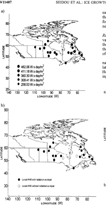
[+o] The retained combinations of explanatory variables for the local ANN models are very different from site to site. Consequently, it is important to investigate whether the characteristics of the input variables have an effect on the best perfbrming variables. Figure 8a presents the mean snow depth on the ground for the ice measurement stations listed in Table 4. Figure 8b presents the list of sites where the best combination of explanatory variables includes snow Similar results are presented lbr rainfall (Figure 9a and 9b) and radiations (Figure 10a and lOb). As for the parameters of the revised Stefàn's law, there seems to be no clear relationship befween the magnitude of a variable, and whether or not it is chosen as an explanatory variable. Figure I I presents the maximum ice rneasurements (Figure 11a) as well as the RMSE of the regional model at these sites (Figure I 1b). The RMSE of the regional model seems to be constant all over the territory. The bias of the regional model is presented on Figure 12. It can be seen on Figure 12 that the regional rnodel slightly underestimates ice thicknesses in the northwestem part of the country where ice thickness is generally large. Conversely, it slightly overestimates ice thickness in the southwestern part of the country, where ice thickness is smaller.

6.4. Limited Comparison of Local ANN Models and Deterministic Model CLIMO

[so] The deterministic model CLIMO was Mënard et al. 12002b) to simulate ice growth at

Figure 7. Increase in RMSE when switching from local ANN with sigmoid activation function for hidden neurons and linear activation function for the output neuron to (top) ANN model with sigmoid activation function for all neurons and (bottom) multiple linear regression model. SEIDOU ET AL.: ICE GROWTH ON CANADIAN LAKES

Ë

o

';

a E o J ',! c o

b )

150

È

Y E l m o _g r * o 1 n

Ë

û 1 m 3 8 û c E d J 6 .to used by . stations E I g a Sum of Degree-days , + + + | , r ' * * - g [ r Sum c,f Degree-dayg nrfrô Ë l.l + 0bseflÉd Srmulaied (ANN) SimulslÊd . r + l ' n n L l ' _Obæryrd û Simulated (ANrl) . * + , t + F h n n J - ' _Y * Srmulaied

Lccal Al.lf.l trodel with sigmoid output function

3 E

Ë

È

I r i îoi 5i, 0;-i . l o i .

'-ral-.-l--l----r

1 0 o f 1 5

w l l 4 0 7 a)

w l l 4 0 7

the local ANN rnodel respectively gave an RMSE of

14.10 and 14.31 cm, which is l3o and 15% higher than

CLIMO. Both models performed better than CLIMO

when simulating ice growth at station YFL (Fort Reliance)

on the data of years 197 7 - I 990. The RMSE was I 7. I 0 crn for

revised Stefan's law and 16.78 cm for the local ANN model,

slightly lower than the 18 cm obtained with CLIMO. Despite

the much higher complexity of the deterministic model, its

performance is comparable to those of the local ANNs and

RSL. I 40.61 cm i 31,45cm a 22.æcm r 13.13cm . 3.97cm 140 130 120 110 100 90 80 r-orcrruoe (W) ê - . < - + ' ' È

a locrlANtl $ih smw fr il* grflnd âs inplt

il LùralANN wiltro{tr sw m ihe Eolld âs inpll

110 100 q) 80 uolcrruoe (W)

Figure 8. Effect of the statistical characteristics of input variables on the best performing solution: (a) mean snow depth on the ground during the ice growth period and (b) usage of snow depth on the ground as explanatory variable by local ANN models.

YZF (Great Slave Lake-Back Bay) for the years 1960-i991, and at station YFL (Great Slave Lake-Fort Reli-ance) tbr years 1977 -1990. They obtained an RMSE of 9 cnt at YZF and 18 cm at YFL. Since those stations are included in our database, the results of the two studies were compared. It can be seen in Table 4 that RSL gives a RMSE of 13.73 cm (12.48 cm tbr the local ANN model) using the "leave-one-out" method on the data of the years 1958-1996 and 2002-2003 at station YZF. When sirnulated on the same period than CLIMO (years 1960 1991) using the leave-one-out procedure, RSL and

SEIDOU ET AL.: ICE GROWTH ON CANADIAN LAKES

u ts tr J u t F

)

70 U o ts J | 1 . 7 4 m m | 1.33 mm a 0.92 mm r 0.5'1 mm , 0.10 mm g 3 ts F J 120 110 100 90 80 rolcruoe (W) 70 60 140 130 120 110 100 90 80 7a 60 r-ollcrruoe M)

Figure 9. Eftbct of the statistical characteristics of input variables on the best perfbrming solution: (a) mean daily rainfall during the ice growth period and (b) usage of rainfàll as explanatory variable by local ANN models. ...^-,Érf .-È;s

11*>:::3q

.1 --À'-.r-i1 {

.t*.*"1e;"H,

? -,"..

a tilâIANN $!ith rsidËtr âs iqlt (j LedANllwithodfrinlsll6inp0t

130 1n 110 1m 90 80

lorcrruoe (W) 70 60

140 130 120 "0,-oJfr"oJ?*,

*

70 60

Figure 10. Effect of the statistical characteristics of input variables on the best perfonning solution: (a) mean sum of solar radiation during the ice growth period and (b) usage of radiation as explanatory variable by local ANN models.

6.5. Regional ANN Model

[sr] The perfomance criteria for the five best combina-tions forthe regional ANN model are given in Table 6. The best combinatiorl (in terms of RMSE) to explain ice growth at tlre regional level is cornbination 1-5 (D"; Rad,,"+ Rad,;R) lollowed closely by combination 20 (Du: Rad,,"+ Rad"; H., R). The optirnal number of neurons on tle hidden layer was found to be one (as indicated earlier, ANN structures with 1 to 10 neurons on the hidden layer were tested, but only one is retained corresponding to the best perfonnance). The regional model is thus relatively parsimonious since it uses only six palameters: one bias and one weight parameter for

w l l 4 0 7 each ofthe connections ofthe inputs (Rad,"+ Rad" and R) to the hidden neuron, and olle bias and one weight parameter for the connection of the hidden neuron to the output neuron.

[sz] The radiation parameter for the regional model is Radn" + Rad" (a: 1), but the choice to split the radiation value into two parts is justified by the fact that for sorne of the local ANN models, the optimal value of o is lower than l. For example, for station WTL, the optimal value of o was fotrnd to be 0.75 (see Tables 4 and l).

[s:] It was also noticed when rating the different combi-nations of input variables for the regional ANN model that latitude and longitude do not have an influence on the result. However. geographic location has a direct influeuce on all input variables. In other terms, geographic location has an

a) | ffi.fficm | 234.ffi cm | 178.00cm r 12200cm . 66.m cm 2 0 t | . . . . . 1 . . . . . . . . . . l

-rm

1oo tio 11b ioo-'.so-..

60

LONGITUOE W) b) 90. 70 ô0 | 2009cm | 1 9 . 1 8 c m ) 18.27 cn | 17.36cm | 16.45 cm )(\t '

T50

100

50

LoNcrruoE (w)

Figure ll. (a) Maximum ice thickness and (b) RMSE of the regional ANN rnodel.

SEIDOU ET AL.: ICE GROWTH ON CANADIAN LAKES

U ts J | 462.06Wxdav/m2 o 411.1BWxdai/m2 | æ0.æwxaay/m1 o 309,tt Wxday/mj o 258,53Wxday/mr u E F J x t i

i

i

I U : l u our

3 soi

i 40r l <t ll I

:3ib.*;

It t

ù\f

1 2 o f 1 5

\ry11407 | 1.75cm o 0.78 cm " -0.20 cm i2 -1.18cm {,* -2.16cn 140 130 LoNGtruoE (w)

Figure 12. Bias of the regional ANN model.

influence on the range of input variables, but not directly on ice growth relationship to input variables.

[sa] An unexpected result in this study is that snow depth on the ground was not identified as an important parameter at the regional level for lake ice growth. This is probably due to the great variability of this parameter in space, which was estimated by interpolation from the weather stations located at several kilometers.

[s:] To illustrate the ability of the regional ANN model to reproduce ice growth dynamics simulated ice thickness (using the regional ANN) at station YZF (Great Slave Lake-Back Bay) is presented in Figure 13. It can be seen that the agreement is excellent.

7. Conclusions

[se] It is shown in this paper that artificial neurai networks can be valuable altematives to complex thermo-dynamic lake ice growth models, especially when dala is not available in sufficient quantity and quality. The performances of tlre proposed ANN models were fairly good when compared to that of the deterministic Cana-dian Lake lce CLIMO. They also offered much more flexibility than the Stefan's law and were able to trans-pose information on ice growth dynamics from monitored

w l t 4 0 7

sites to unmonitored sites or periods using only six weight and bias parameters. They also reproduced various ice growth pattems with a t'ew easily obtained meteoro-logical data.

[sr] The methodology presented in this paper is of the greatest importance for Nordic hydrologists since no oper-ational model of lake ice growth exists for ungauged sites. This gap needed to be addressed for several reasons: a practical rnodel of lake ice growth can help assess the impact of climate change on lake ecosystems, which is a topic of great concern nowadays. It can also be used to estimate the arnount of water that is lost as ice left on the banks of hydroelectric reservoirs during winter operation, which may be important for large annual reservoirs in northem countries.

[sa] The main limitation of the work presented in this paper is that it applies only to the ice growth period. In other empirical rnodels, a combination of freezing degree-days and n.relting degree-degree-days have provided good results in modeling the whole duration of the ice cover [e.g., Thompson et al., 2005). The extension of the developed rnethod to the whole duration of the ice cover using a single ANN rnodel is a challenging problern because of the differences in the two processes to be rnodeled. The leaming perfonnance of the ANN may hence be reduced. A possible alternative solution is to train an ANN model for the growth phase and another one for the decay phase.

Appendix A: Solar Radiation at the Top of Atmosphere

[:::::::::::::::::::::::::::::::::::::::::::::::::::::::::::::::::::::::::::::::::::::::::::::::::::::r] These relations are obtained from the Solar Radia-tion Monitoring Laboratory [2004]. On average extrater-restrial inadiance is 1367 W/m2. This value varies ly t3Yo as the earth orbits the sun.

( A l )

where Ào, is the average Sun-Earth distance, R is the actual Sun-Earth distance depending on the day of the year, and Z the zenith (the angle of the sun relative to a line perpendicular to the Earth's surface) which depends on the declination of the Earth, latitude and solar tirne. If one notes n the Julian day, Eq, (equation of time) the variation in minutes of the solar time (f.,1,,.) compared to the standard time (76,) during the year. w the solar hour angle (in radians), Longç,.o1the longih,rde of the cenhal meridian line SEIDOU ET AL.: ICE GROWTH ON CANADIAN LAKES

U F F

1 : 1 36?(*)'*.o,(Z) _{KW lm2}

Table 6. Perl'omrance Criteria of the Resional Model for the Five Best Combinationso

Combination of Meteorological Vari ables RMSE (RSL), cm (RSL) RMSE (ANN), cm RRMSE (ANN) NASH (RSL) N A S H (ANN) r, RRMSË (ANN) (RSL) BIAS BIAS (RSL), (ANN) cm cm l 5 20 l 9 1 4 l 8 2 5 . 0 8 2 5 . 0 8 2 5 . 0 8 2 5 . 0 8 2 5 . 0 8 0 . 6 5 0 . 6 5 0.65 0.6-5 0 . 6 5 1 8 . r 5 I 8 . 1 7 1 8 . 1 7 1 8 . 1 9 18.24 0 . 8 2 0 . 8 2 0 . 8 2 0 . 8 2 0 . 8 2 0 , 4 2 0 , 4 2 0 . 4 7 0 . 1 2 0 . 4 2 0 . 4 3 0.43 0 . 4 3 0.43 0.43 0 . 6 5 0.65 0 . 6 5 0 . 6 5 0 . 6 5 0 . 8 2 0 . 8 2 0 . 8 2 0 8 2 0 . 8 1 - 0 . 1 5 0 . 6 5 * 0 . 15 0 . 5 6 - 0 . 1 5 _{0 . 1 2} - . 0 . _{1 5 t . 2 3} 0 . 1 5 - 0 . 4 8

uOne _{neuron on the hidden layer and perfomrance indices obtained during the leave one out cross-validation procedure. Note longitude and latitude are}

not listed as explanatory variables because it was fbund that they have no intluence on the output ofthe regional model.

\ry11407 SEIDOU ET AL.: ICE GROWTH ON CANADIAN LAKES

1 8 o l

.

g

rl1

lfff{ff{ruli${riif$r|$iigsrfi#iis

1958 1964 1970 1976 1982 1988 1994 [-;ô;;--- ; sili;bd iÂNNt :

Figure 13. Simulated and observed ice thickness at station YZF.

of the tirne zone and Lon5g,n, the longitude of the point of calculation, we have the following approximations:

f & ) ' - l . 0 0 0 l l + 0 . 0 3 4 2 2 1 * . o r l ' z n ' \ + 0 . 0 0 1 2 8 0 \ R , / \ l 6 s / - s i n ( z ' 3 ) + 0 0 0 0 7 1 e * . o . ( + o 3 ) F 0 . 0 0 0 0 7 7 \ J ô ) / \ J 6 5 / . L n \ + s r n ( 4 ; r * I ( ^ 2 ) \ J O ) / c o s ( Z ) : s i n ( / ) s i n ( d ) * c o s ( / ) c o s ( d ) c o s ( u , ) ( A 3 )

tt:23.45."i"(2"?!ff)

_tool

. . . _ _ * ( t 2 T , , a , . ) l 2 , . E q t . ,

T,uru, - Tlocal *;0 * (Long,n, - Long1,,,.,1)/15

Notation

e'n ANN output vector of the mth layer. B^ ANN bias vector of the connections fonn the

(m-l)th layer to the (m)th tayer.

C bias parameter of the rnodifred Stefan's law.

C,, heat transfer coeffrcient from ice to air.

Da sum of degree-day from the date of ice cover fomration.

Ds sum of degree-day from the first below zero remperarure.

ANN transfer function of the mth laver. ice thickness.

rnean ice thickness.

kth ice thickness in the data set.

estimate of the kth ice thickness in the data set. on-ground snow depth.

lnean on-ground snow depth. coefficient of Stefan's law.

average rainfall during the ice growth period. snm of solar radiation of days with precipitation (snow or rainfall).

Rad," sum of solar radiation of days without precipitation (snow or rainfall).

(A5) [l''n ANN weight vector of the connections form the (m-l)th layer to the (m)th layer.

[oo] lcxnowledgments, The financial support provided by the l A f r \ N a t u r a l S c i e n c e s a n d E n g i n e e r i n g R e s e a r c h C o u n c i l o f C a n a d a \'--l _{(NSERC), Hydro-Quebec, the GEOIDE network, and the Nodhem Study}

Center (CEN) at Laval University is gratefully acknowledged. This researclr was partly carried out while the second author was on sabbatical leave at the National Engineering School of Tunis (Tunisia). The authors would like to thmk the associate editor and three anony-mous reviewers whose comments helped improve the quality of the original manuscript.

(47) References

Beltaos, S. (1,995'1, River lce Jarnr, Water Resour. Publ., Highlands Ilanch,

Colo.

Canadian [ce Seruice (2005), Ice thickness data sets, http:/iice-glaces. ec.gc.ca, Ottowa.

Cannon, A. J., and P. H. Whitfield (2002), Downscaling recent streantllow conditions in British Columbia, Canada using ensemble neural nehvork models, -/. Ilydrol., 25.9, 136- 151.

Coulibaly, P., and F. Anctil (1999), Real time short tem natural walers inflow forecasting using recurrent neurel networks, in Proceedings of

lntenntional Joint Conference on Neural Networks, 1999. IJCNN '99,

vol. 6, 3802-3805, {EEE Press, Piscataway, N. J.

Coulibaly, P, F. Arctil, and B. Bobée (2000), Daily reseruoir inflow fore-ca-sting using artificial neural networks with stopped training approach, .1. I'lvdrol., 2 3 0, 244 -757. 1 4 o f 1 5

4t

H r 1-Hi Hi

Us

H S

k

Â

Rad. I i ^ t -/ n + 7 \ - l a . 2 s i n [ n - ) t 3 n < t 0 6 + . o r ; n ( o n - l o 6 ) ' o t . n < t 6 6 \ 5 e ) -- 6 . 5 s i n (^ ' . ] u u ) t 6 7 < n < 2 4 6 \ 8 0 / * / n - ) 4 7 \ t 6 . a s i n ( n * ) 2 4 7 < n < 3 6 5

wt 1407

Cybenko, G. (1989), Approximation by superposition ofas sigmoidal func-tion, Math. Control Signals S.)rt, 2, 303-314.

Duguay, C. R., G. M. Irlato, M. O. Heffries, P Ménard, K. Morris, and W. R. Rouse (2003), lce covers variability on shallow lakes at high altitudes: Model simulation and obseruations, IIydrcl. Processes, 17,3465-3483. Fang, X., C. R. Ellis, and H. G. Stefan (1996), Simulation and observation

of ice formation (lieeze-over) in a lake, Cold Reg. Sci. Technol., 24, t 2 9 - 1 4 5 .

Flato, G. M., and R. Brown (1996), Variability and climate sensitivity of land fast arctic sea ice, J. Geophys. Res., 101,25,767-25,771. Hagan, M. 1l (1996), Neural Nehuork Dargn, I'WS, Boston.

Hewett, R. (2003), Data mining for generating predictive models of local hydrology, Appl. Intell., 19, 157 -170.

Homik, K., M. Stinchcombe, and H. White (1989), Multilayer feed-fbrward neural networks are universal approximators, Neural Networks, 2, 359-366.

Lenormand, F,, C. R. Duguay, and R. Gauthier (2002), Development ofa historical ice database for the study ofclimate change in Canada, Hydrol. Processes. I 6. 3707 -3'122,

Liang, R. H., and Y. Y Hsu (1994), Schedulilg ofhydroelectric generation using artilicial neuml networks, lEE Proc., Part C, 145,452-458. Lock, G. S. H. (f990), The Grou,th ond Deca1, oflce,CarnbndgeUniv.

Press, New York.

MacKay, D. J. C. (1992), Bayesian interpolation, Neural Comput., 4, 4 t 5 - 4 4 7 .

MacKay, D. J. C. (1995), Bayesian non-linear modeling with neural net-works, reporl, Cambridge Programe for Ind., Cambridge, U. K. Matousek, V (l 984). Regularity of the freezing up ofthe water surface and

heat exchange between water body and water surface, paper presented at IAHR lntemational Synrposium on lce, Int. Assoc. ofHydraul. Eng. and Res. Hamburg, Germany'.

Ménard, P., C. R. Duguay, G. M. Flato, and W. R. Rouse (2002a), Simulation of ice phenology on Great Slave Lake, Northwest Teritories, Canada, llydrol. Prccesses, 1 6, 3691 -3706.

Ménard, P, C. R. Duguay, G. M. Flato, and W. R. Rouse (2002b), Simula-tion ofice phenology on a large lake in the Mackenzie Rivc'r basin, Proc. Annu. Meet. Eastem Snow Conf., 59th(3),12.

Michel, B. (1971), fiiinter Regime ofRiters and Lakes, Cold Reg. Res. and Eng. Lab., Hanoveq N. H.

Olsson, J., Cl. B. Uvo, md K. Jinno (2001), Statistical atmospheric dowr-scaling of short-tem extreme minfall by neunl networks, Phys. Chent. Earth. Part B. 26.695-700.

Omstedt, A. (1985a), On supercooling and ice lbmation in turbulent sea-water. J. Glar:iol. 31.272-280.

Omstedt, A. (1985b), Modeling fizil ice and grease ice fomation in the upper layers of the ocean, Cokl Reg. Sci. Ibchnol., l I , 87 -98. Ouarda, T. B. M. J., H. Gingras, S. Hamilton, H. Ghedira. and B. Bobée

(2003), Estimation of streamflow under ice, paper presented at the l2th

w l l 4 0 7 Workshop on the Hydraulics of Ice Covered Rivers, Committee on River lce Processes and the Environment, Canadian Geophysical Union (CGU-HS), Edmonton, l9-21 June.

Schulyaliovskii, L. G. (Ed.) (1966), Manual oJ'lce-Fornotion Forccasting for Rivers and Inland Lakes, Isr. Prog. for Sci. Trmsl., Jerusalenr. Shamseldin, A. Y. (1997), Application ofneural network technique to

rain-1àll-runoff modeli ng, J. IIy dro l., 1 9 9, 27 2 - 29 4.

Shen, H. T., and L. A. Chiang (1984), Simulation ofgrowth and decay of river ice cover, J. Hydraul. Eng., 110,958-971.

Shen, H. T., and C. F. Ho (1986), 'lwo-dimensional simulation of ice cover fomation in a large riveq paper presented at IAHR Ice Symposium, lnt. Assoc. of Hydraul. Eng. and Res., Iowa City, lowa.

Shen, H. T., H. H. Shen, and S. M. Tsai (1990), Dynamic transport ofriver ice, J. Hydruul. Rcs.,28,659-671.

Shen, H. T., D. S. Wang, and A. M. W. Lal (1995), Numerical simulation of river ice processes, J. Cold Reg. Eng., 107, 107-118.

Solar Radiation Monitoring Laboratory (2004), Solar radiation basics, re-port, Univ. ofOreg., Corvallis. (Available at http://solardat.uoregon.edr/ SolarRadiationBasics.html),

Stefan, H. G., and X. Fmg (1997), Simulated climate change effects on ice and snow cove$ on lakes in a temperate region, Cold Reg. Sci. Technol., 25, t37 -t52.

Svensson, U., and A. Omst€dt (1994), Simulation ofsupercooling and size disnibution offtazil ice dynamics, Cold Reg. Sci. Technol.,22,221 -233. Svensson, U., L. Billfalk, and L. Hammar (1989), A mathematical model of border-ice îomation in rivers, Cold Reg. Sci. Technol., 16, 179-189. The lr{athrvorks (2005), Neural Nehvork Toolbox. user's guide, version 5.

Natick, Mass. (Available at http:,//www.mathworks.com./accessftrelpdesk/ help/pdf docÂrnet/nnet.pdl;

'lhompson,

R., et al. (2005), Quantitative calibration ofremote mountain-lake sediments as climatic recorders of air temperature and ice-cover dumtion. lrct AntarcL Alp. Res., 37(4),626-635.

Xiao, R., and V. Chandræekar (1l997), I)evelopment of a neuml network based algorithm for rainfall estimation from radar observation, lE f Trqns. Geosci. Remote SeLt., JJ, 160-171.

Zhang, S. P. H. Watanabe, and R. \hmada (1994), Prediction ofdaily water demand by neuml networks, in Stochastic and Stotistical Melhods in Hydrologt and Environmental Engineering,tol- 3, edited by K. W Hipel et al., pp. 217 *227, Springer, New York.

L. Bilodeau and P Bruneau, Hydro-Québec,855 Ste-Câtherine Street

East, l2th Flooq Montreal, QC, Canada H2L4P5.

M. Hessami. T. B. M. J. Ouarda, O. Seidou, and A. St-Hilaire, INRS-ETE, 490 me de la Couronne, Quebec. QC. Canada GIK 949. (ousman [email protected])

SEIDOU ET AL.: ICE GROWTH ON CANADIAN LAKES