A behavioral simulation model of forecasting and production scheduling in a datacommunications company

HD28

.M414 Dewey

WORKING

PAPER

ALFRED

P.

SLOAN SCHOOL

OF

MANAGEMENT

^A

BEHAVIORAL SIMULATION MODEL OF FORECASTING AND PRODUCTION SCHEDULING

IN A DATACOMMUNICATIONS COMPANY,^ by John D.W. Morecroft WP-1766-86

MASSACHUSETTS

INSTITUTE

OF

TECHNOLOGY

50

MEMORIAL

DRIVE

CAMBRIDGE,

MASSACHUSETTS

02139

D-3807

^A

BEHAVIORAL SIMULATION MDDEL OF FDRECASTING AND PRDDOCTION SCHEDULING

IN A DMACOMMUNICATIONS COMPANY

^

by

Jolin D.W. Morecroft WP-1766-86

D-3807

A

BEHAVIORAL

SIMULATION

MODEL

OF

FORECASTING

AND

PRODUCTION

SCHEDUUNG

IN

A DATACOMMUNICATIONS

COMPANY

by

John D.W. Morecroft

System

Dynamics

Group

Sloan School of

Management

Massachusetts Institute of

Technology

Cambridge

MA

D-3807

A

BEHAVIORAL

SIMULATION

MODEL

OF

FORECASTING

AND

PRODUCTION

SCHEDUUNG

IN

A

DATACOMMUNICATIONS

COMPANY

Abstract

The

paper

describes a behavioral simulation

model

of forecasting

and

production scheduling in a datacommunications

company.

The

model

allows

you

to think about the different 'players'

whose

choices

and

actions

regulate orders

and

production.

There

are business planners (who provide

forecasts), factory schedulers, expediters,

customers

and

account

executives.

You

step into their shoes.

You

examine

their responsibilities, their goals

and

incentives

and

the sources of information that attract their attention -- _{all with the intention of understanding the logic behind}

their choices

and

actions.

Then

you

stand

back

from the detail and, with the help of diagrams

and

simulations, you explore

how

the players interact

and

cooperate,

and

how

the factory balances supply

and demand.

D-3807

INSIDE

THE

FACTORY

Imagine youself as the

manager

of a factory that

produces

workstations,

PBXs,

key

systems and

other datacommunications equipment.

Your

factory

has

been

criticized recently for slow deliveries.

The

delivery interval of

workstations ranges from six

months

to

one

year,

much

longer than major

competitors.

The

problem

is not improving.

You

begin searching for an

explanation.

Many

ideas

come

to mind.

One

could argue that the factory's long delivery intervals are

due

to errors in the sales forecast.

You

could obviously run the factory better

and

make

deliveries on time if you

were

given accurate

forecasts. But

you

realize that forecasts will

never

be

accurate,

particularly in the

datacommunications

market

where

technology is

causing products

and

prices to

change

rapidly. Alternatively,

one

could

argue

that the factory's long delivery intervals are

due

to inflexible

suppliers

who

can't expedite parts

and

materials if the factory suddenly

needs

more. But, on reflection,

even

this

argument

is not entirely

convincing.

Suppose

for

example

that a large

shipment

of parts

and

materials arrives unexpectedly,

enough

to

make

50

extra workstations.

What

would

you

do

with workstations,

where would

you

send

them?

Let's

say there are

100 customers scheduled

to receive a workstation this month.

On

average

they've waited say eight

months

for delivery, but

now

their

machines

are in the shipping dock, ready to

be

loaded onto a delivery

despite the eight

month

delivery interval, the factory cannot ship the 50

extra workstations,

because

the order

book

doesn't

show

another 50 customers

who

are expecting to receive a workstation this month. Instead

it

shows

100 customers

who

are expecting delivery this month,

and

several

hundred customers

who

are expecting delivery during the next twelve months. It's not a simple matter to ship the extra workstations

early -- _customers

_{must be}

_{informed of early deliveries, so}

_must

_{the sales}

and

field support organization. Moreover, the factory has to adjust the

production schedule to account for early deliveries.

As

you

think about it, the factory's

problem

is not with late deliveries (since

most customers

receive their workstations

on

the promised date) but, instead, with slow deliveries -- _{workstations are shipped on time,}

but the

agreed

delivery interval is too long!!

You

seem

to be gridlocked.

How

does

the factory get out of this delivery situation, and, perhaps

more

important,

how

does

it avoid

extended

delivery intervals in the first

place?

To

help explore these questions a simulation

model

has

been

developed of a

factory, customers

and

account executives.

The

model

allows you to think

about the different 'players'

whose

actions

and

choices regulate orders

and

production.

There

are business planners

(who

provide forecasts), factory

schedulers, expediters,

customers

and

account executives.

You

step into their shoes.

You

examine

their responsibilities, their goals

and

incentives

D-3807

and

the sources of information that attract their attention -- _{all with the}

intention of understanding the logic behind their choices

and

actions.

Then

you

stand

back

from the detail and, with the help of

diagrams and

simulations, you explore

how

the players interact

and

cooperate,

and

how

the factory balances supply

and demand.

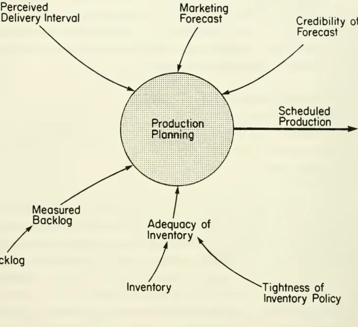
Production Planning

and

Factory Scheduling

Consider

first production planning, which is a multilayer process that

consolidates information from forecasters, from product

managers

and

from the factory. Figure 1

shows

the information entering the production

planning policy.

An

important input is the market forecast

based

on the marketing staff's

business plan.

The

business plan starts from an estimate of total industry

volume

for all classes of

datacommunications

equipment.

From

historical

data

and

various business

assumptions (new

product introductions, price

changes,

competitor actions,

expected

delivery intervals), forecasters

compute

the

company's expected

share of industry sales. Then, they

multiply industry

volume and

expected share to generate the

company's

sales forecast by product line over a two-year planning horizon.

The

forecasting process is a logical exercise in gathering

and

_processing market information. But as the forecast enters the factory, to be

used

in

production scheduling, it is modified by its

own

credibility (its reputation for accuracy in the factory), by pressures from inventory, delivery interval

Perceived Delivery Interval

Measured

Backlog

Backlog

Marketing

Forecast

Adequacy

of Inventory Credibility of Forecast

Scheduled

Production Inventory

Tightness

of Inventory Policy ^-3Z3'=\B

D-3807

and

backlog. Let's consider

each

of these factors in turn in order to identify the people

most

responsible for modifying the forecast

and

their

rationale for doing so.

Let's begin with the forecast credibility. It is quite

common

in

datacommunications companies

for market forecasts to lack credibility at

the factories.

The

reasons are easy to understand.

The

datacommunications market is in flux.

New

products are introduced almost daily, prices

change

frequently,

new

competitors spring up. Factory

managers

feel that

forecasters simply don't

know

the sales potential of a given product line

(despite their elaborate forecasting methods)

and

therefore, forecasts are often pared-down, to

be

'on the safe side',

and

particularly to avoid the

very visible inventory costs resulting from

excess

production.

What

if the forecast is inaccurate?

How

does

the factory

know

of the

error,

what

source of information

would

reveal the error,

who

would be

responsible for adjusting the production schedule

and would

they

have

the incentives

and

appropriate information to

make

the correct adjustment?

Now

we

are getting into the heart of factory scheduling, stepping into the

shoes

of the schedulers themselves.

The

production schedule is defined over a rolling six-month horizon.

One

can

envisage a planning chart, with

boxes

marked

across

a

page.

The

(say workstations) scheduled for production in the current

month

(in fact

the schedule

may

be

expressed in

weeks

or

even

days, but it

makes

no

difference for this discussion).

The

extreme

right-hand

box

shows

the

number

of units scheduled for production six

months

from now.

The

boxes

in-between

show

monthly scheduled production for

months

2 through 5.

Each month

the planning chart is updated, the current month's

box

"drops off the left-hand side of the chart,

and

a

new

box

'rolls in' on the

right-hand side, rather like the steps on

a moving

escalator.

The number

in the

new

box is the forecast of customer orders six

months

hence.

The

scheduler assigns incoming customer orders to the appropriate box.

To

understand the process, imagine that the factory is trying to deliver on a

three

month

interval.

A

new

customer

order is received (say an order for a

workstation) which is

due

for installation

and shipment

in three

months

time.

The

scheduler looks in the planning chart for the box corresponding

to

month

3.

He

finds a workstation that is scheduled for production

and

assigns the

customer

order to it.

That

particular workstation is

now

'earmarked' for a customer and cannot be assigned again.

The

process

works

smoothly as long as the original forecast

was

accurate.

But

what

happens

when

the forecast is low? Again the factory is trying to

deliver on a three

month

interval.

Based

on the forecast, 1 00 workstations

have

been

scheduled in the time slot three

months

hence. But orders for

D-3807

exactly as before, until the entire box is assigned.

Then

he assigns the

remaining 'unexpected' orders to the next available

box

-- _{in other}

_words

to a later time slot. Having

done

so, he then informs the salesforce that

workstations are available only on an extended delivery interval.

Because

of the long production planning horizon, schedulers can almost always find an

open

production slot for a

new

customer order.

When

a

customer

order

has

been

assigned a production slot, the scheduler has

done

his job.

So

schedulers,

who

are 'close' to the

customer

order backlog,

and

therefore the first people in the

company

to

see

when

the forecast is too low,

have

no incentive to argue for higher production, as long as production slots

remain open.

The

same

logic

works

in reverse.

When

the forecast is optimistic

and

production is scheduled in excess of

customer

orders, schedulers begin to

find early time slots for

new

customer

orders.

So

a

scheduler might

receive an order for

a

workstation

due

in three months, but finds he can

assign it to an

open

production slot only two

months

hence.

The

scheduler

has

done

his job, so again, although he

knows

the factory is producing the

wrong

amount

(too

much)

he has no

incentive to

argue

for a lower

production plan.

However,

in this case, pressure to reduce the production

plan will eventually

come

from finished inventory. If

customers

are unable

to take

an

early delivery , then products awaiting

shipment

will

accumulate

in finished inventory

and

signal a factory

manager

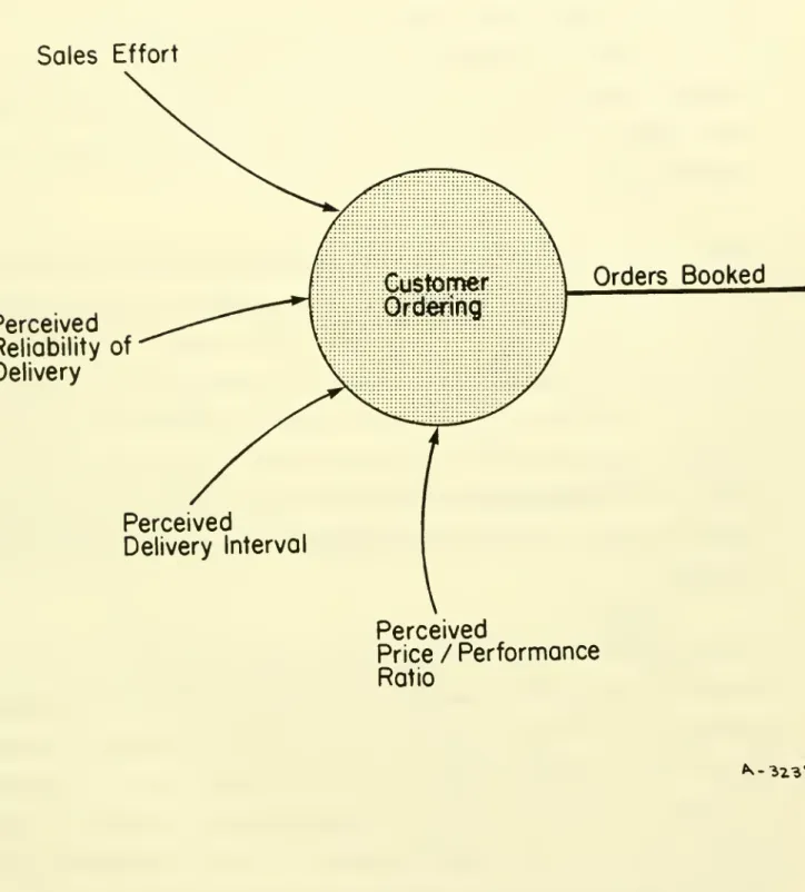
to curtail

Customer

Ordering

Figure 2

shows

the influences on

customer

ordering. Sales effort is the

principal influence,

because customers must

learn about the

company's

products before they will

even

consider purchase. Then,

once

the customer is

aware

of the product, traditional factors such as price/performance

and

delivery interval

become

important.

Let's

suppose

for the

sake

of simplicity that the price/performance of a

given product line is constant,

and

that sales effort (which you can think of

as

the

number

of hours per

month

the salesforce

spends

with

customers) is constant.

How

do customer

orders vary with

changes

in

delivery interval? Think

about

this question from the perspective of

account executives as they contact potential customers.

Suppose

that

account

executives

have

been

selling workstations on a three

month

delivery interval.

Then

factory schedulers

announce

that the interval

must

be

extended

to five months.

Account

executives can still sell workstations

on the five

month

interval, but they will take longer to find a

customer

who

is willing to wait the extra

two

months.

The

net effect is that

customer

orders decline as the interval rises,

and

conversely, that

D-3807

11 Sales Effort Perceived Reliability of Delivery Perceived Delivery Interval

Orders

Booked

Perceived

Price /

Performance

Ratio ^-^Z3tB

DYNAMICS

OF

PRODUCTION

SCHEDUUNG AND

CUSTOMER

ORDERING

If

one

accepts that customers, planners

and

schedulers

behave

as

described above, then

how

do

they interact?

To

answer

this question let's first visualize the feedback loops connecting the 'players'.

There

are two

important loops.

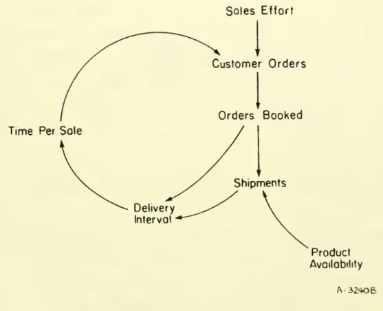
Figure 3

shows

a negative feedback loop connecting customers' ordering to

the

company's

deliveries. Consider the loop's operation if product suddenly

becomes

less available (the factory shuts

down,

or there is a

transportation strike).

Shipments

decline, causing delivery interval to

rise.

When

the delivery interval rises it takes

more

time for salespeople

to

make

a sale, so that, for any given sales effort,

customer

orders decline

and

the total

number

of orders

booked

stabilizes.

Here

is a self-regulating

demand

mechanism

that brings customer orders into an exact balance with

shipments.

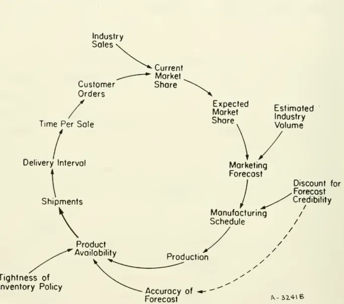
Figure 4

shows

a positive feedback loop connecting cutomers' ordering to

forecasting, production scheduling

and

shipping. This loop can readily

generate

self-fulfilling forecasts,

as

the following

argument

shows.

Suppose

that production declines

due

to a previously inaccurate forecast.

A

decline in production quickly curtails

shipments (assuming

that the factory

keeps

very little finished inventory).

When

shipments

fall, the

delivery interval rises, time per sale increases

and customer

orders fall.

D-3807

13

Time Per Sale

Delivery Interval Sales Effort Customer Orders Orders Booked Shipments Product Availability

Figure 3: Negative

Feedback Loop

Connecting Customers'

Industry

Sales

Customer Orders

Time Per Sale

Current Market Shore Expected Market Stiare Estimoted Industry Volume Delivery Interval Shipments Product Availability Tightness of Inventory Policy Marketing Forecast Discount for Forecast Credibility Manufacturing / Schedule / / / / / Production y' k- 51+lB Accuracy of -*-Forecast

Figure 4: Positive

Feedback Loop

Connecting Customers'

D-3807

15

market share, as it is

based

largely on historical data.

Because

expected share falls, the marketing forecast is further reduced

and

so too is the

production schedule

and

the production rate.

The

initial product shortage

therefore feeds

back

to reinforce itself.

In the real

system

the two loops are combined.

We

can use simulation to

understand

how

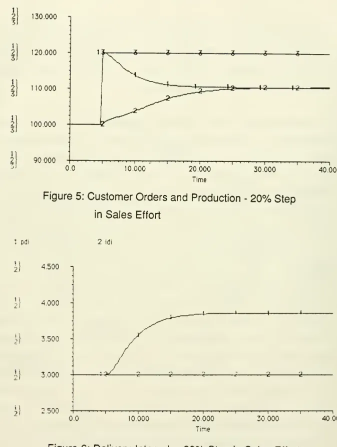
they operate. Figure 5

shows

the system's response to a

one

time twenty percent increase in sales effort (the reader should note

that, in the factory model, sales effort is 'exogenous' -- the

modeler

is free to set sales effort at any value he thinks appropriate. In this case,

we

know, from the sales planning

and

control

model

described in D-3806, that

sales effort in a datacommunications

company

can vary widely

depending

on the terms of the compensation

scheme.

So

a simulation experiment that

assumes

a large, twenty percent, increase in sales effort is certainly plausible).

The

model

starts in equilibrium, with

customer

orders (-1-)

and

production (-2-) of 100 units per month.

When

sales effort increases,

orders (-1-) increase correspondingly to a

peak

of

120

units per month.

However,

as time

goes

by, orders (-1-) are gradually

eroded

until they

settle at a

new

equilibrium of

110

units per

month

--

_an

_{increase of 10}

units a month, but only half the possible increase.

Meanwhile

production

(-2-) increases slowly

and

steadily until it exactly equals

customer

orders (-1-). But

why

are orders permanently

depressed?

As

figure 6

shows, the

immediate cause

is delivery interval (-1-) which rises from 3

120.000

no000

100.000

90 000

Time

Figure 5:

Customer

Orders

and

Production -

20%

_Step

in Sales Effort 40.000 1 pdi 2 idi 2} 4.500 4000 3,500 3.000 ^} 2 500 40 000

D-3807

17

willing to place an order

when

the interval is extended.

But

why

doesn't the interval fall

back

to three

months once

the surge of

orders has

passed?

To

answer

this question

we

need

to look closely into

the 'mechanics' of forecasting

and

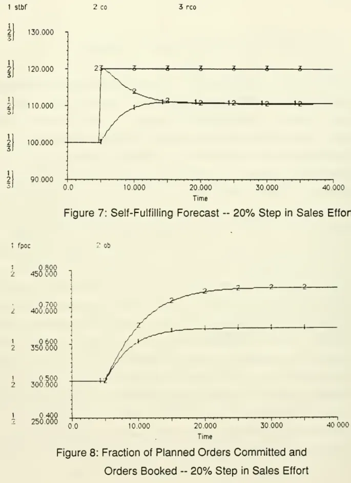
scheduling. Figure 7 provides part of the

story.

When

orders increase unexpectedly, the forecast increases too, but only gradually.

As

customer

orders (-2-) decline (due to increased delivery

interval), the forecast (-1-)

changes

course. Instead of continuing

upward

toward reference

customer

orders (-3-), (the value that

customer

orders

would

achieve if delivery interval

were

fixed at three months) it

homes

in

slowly on the final

and depressed

value of orders. In other words, the

forecast is self-fulfilling.

The

only

way

out of this trap is to schedule

production in

excess

of the forecast. But there is

no

pressure on the factory schedulers to do so. Figure 8

shows

why.

When

customer orders are

unexpectedly high, the schedulers simply assign the

excess

orders to the earliest convenient slot in the pre-planned manufacturing schedule.

So

the

surge of orders is

absorbed

by

consuming

a larger proportion of the

pre-planned schedule (-1-) instead of expanding the schedule by adding

the

excess

orders to the forecast.

As

a

result, orders

booked

(-2-) rise

too high

-

higher than they should if deliveries are to remain competitive -- _{yet, at the}

same

_{time, the illusion exists in the factory that the}

customers

are satisfied, since

each

customer

order is

assigned

a

1 2 3J 130.000 120,000 10.000 100.000 90.000 0.0 2J

_N

4^ ^ 10 ID 10.000 20.000 Time -p-i r— 1 1 1 1 p 30.000 40.000

Figure 7: Self-Fulfilling Forecast --

20%

_{Step in Sales Effort}

1 Tpoc 2 Ob 2 800 ^ 450 000 1 0,700 400.000 t 600 2 350 000 1 0.500 2 300.000 400 250.000 10.000 20.000 Time 30 000

Figure 8: Fraction of Planned Orders

Committed

and

Orders

Booked

--

20%

_{Step in Sales Effort}

D-3807

1

9

agreed to.

The

illusion is easily sustained,

because

the factory

keeps

the

salesforce up-to-date

on

the earliest time slots available in the

production schedule, so salespeople tend to find

customers

who

are

satisfied with the factory's schedule.

SELF-SUPPRESSING

DEMAND

The

simulations

above

show

that the factory's forecasting

and

scheduling

policies fail to regulate delivery interval

-

instead they allow the

interval to drift

upward

whenever

the forecast is too low.

As

a result, the factory can inadvertently suppress orders for its growing product lines.

To

understand

how, consider the

case

of a

new

product line

which

is

attracting a growing proportion of sales effort. Think

back

to simulations

of the sales planning

and

control

model

in D-3806.

Customer

orders can

grow

very quickly.

They

can double in six months, not

because

customers

are

stampeding

to buy, but instead

because

the salesforce is anxious to

sell! With

such

rapid salesforce-induced growth it's

easy

for the sales

forecast to

be

too low, not just for a

week

or a month, but for six

months

or a

whole

year. With a low forecast, the factory's scheduling policies

allow delivery interval to drift upward.

The

interval will continue to drift

upward

until it is high

enough

to deter

customers

from buying

and

salespeople from allocating still

more

time to selling the product.

Customer

orders will therefore stop growing.

So

the interaction of factory

scheduling

and

salesforce time allocation will suppress

demand

for the

POLICIES

TO

CONTROL

DELIVERY INTERVAL

To

prevent the problem of self-suppressing

demand

the factory

needs

to

manage

the delivery intervals of its different product lines, to ensure the intervals remain competitive.

The

idea of

managing

intervals here

means

more

than

implementing

a special interval reduction program.

Such

programs

typically occur only

when

intervals are so high that they attract

senior

management

attention.

By

then the

image

of extended intervals is

already well-established with

customers

and

with the salesforce,

and

many

potential orders

have

been

lost.

Managing

intervals

means

establishing a routine policy, at the level of schedulers

and

planners, that rapidly detects systematic bias in the forecast

and

compensates

for it by

scheduling production in

excess

of the forecast.

Two

possible interval control policies are described

and

simulated below.

Monitoring

and

Control of Excess Orders

The

first policy requires schedulers to monitor

excess

orders

and

use

them

to adjust the forecast.

An

example

is helpful to explain.

Suppose

the factory is planning production of workstations over

a

six-month horizon

and

is

now

delivering workstations with

an

interval of three

months

(competitive for the industry). In the current

month

the factory receives

120

orders for workstations,

due

for delivery three

months

hence.

The

scheduler looks at planned orders three

months

into the planning horizon.

He

finds only

100

workstations scheduled for that

month

-

100 being the forecast of orders generated three

months

ago, at the start of the planning

D-3807

21

process. With the present procedure the scheduler puts the 20

excess

orders into next month's time slot

and

then informs the salesforce of the

schedule change. With the

proposed

system

the scheduler would, in addition, count-up all excess orders (all orders

whose

scheduled delivery

date is greater than three

months

--

20

in this case)

and

communicate

the

number

to production planners.

Each month

the planners

would add

the excess orders to the current month's forecast. ( This procedure

may seem

to result in double scheduling

because

the schedulers first assign the 20 excess customer orders

and

then the planners

add 20

units of production to

the forecast. But in fact a customer order is scheduled once,

and

once

only,

by the scheduler.

The

planners use the

20 excess

orders as a guide for

increasing the forecast. Their concern is with planning the

volume

of

future production, not with scheduling individual

customer

orders).

The

same

procedure could also be

used

to reduce the production plan to

compensate

for a high forecast. In this

case

the scheduler would count-up

all planned orders in the time slots before

month

three that

have

not

been

assigned a

customer

order.

He

would

then

communicate

this

number

of excess planned orders to production planners.

The

planners would subtract the

excess

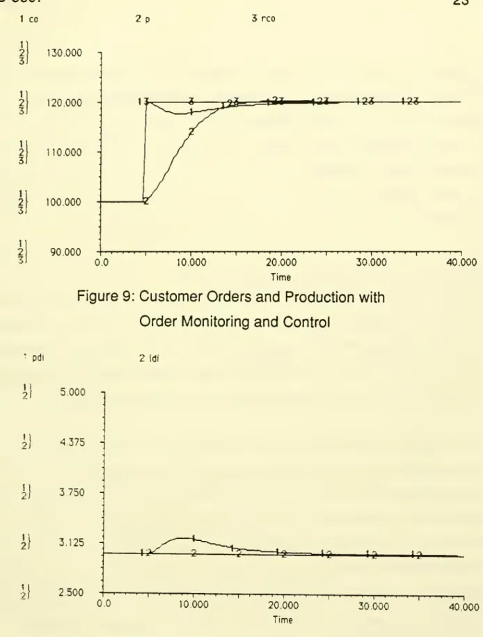
orders from the current month's forecast.

Figure 9

shows

a simulation of the order monitoring

and

control policy,

with

a 20

percent increase in sales effort.

The

reader should

compare

figure 9 with figure 5.

As

before,

when

sales effort increases,

customer

orders (-1-) increase correspondingly to

a

peak

of

120

units per month.

After the

peak

however, orders (-1-) decline only slightly,

and

then settle

at an equilibrium of

120

units per month. Meanwhile, production (-2-)

increases slowly until it exactly equals

customer

orders.

Figure 10 shows, that with the

new

policy in operation, delivery interval

(-1-) stays close to three months, despite the surge of orders.

So

the

factory

no

longer

suppresses

demand

due

to

extended

intervals.

The

improvement

in delivery performance occurs

because

planners

expand

the

production schedule

more

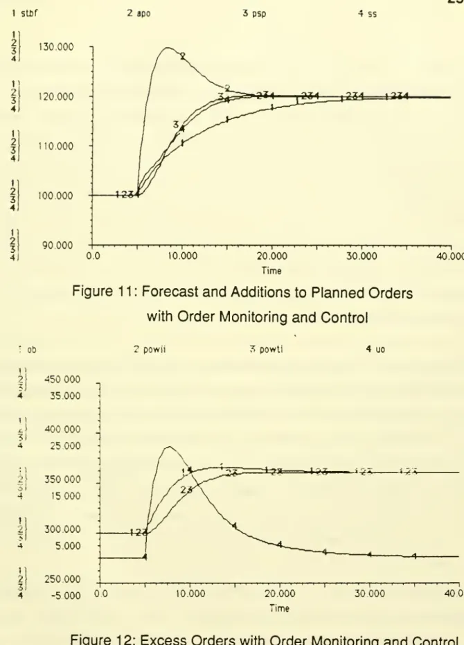
quickly than the forecast alone would suggest.

Figure 1 1

shows

what

is happening.

From

month

to

month

5, the forecast

(-1-) is steady at

100

units per month. In

month

5 (the time

when

customer

orders increase) the forecast (-1-) starts to rise, but only

gradually

because

forecasters

do

not anticipate (by assumption) the step

increase in sales effort that is causing the extra

demand.

By month

10, the forecast (-1-) has risen to 110 units per

month

(in other words, in

month

10, forecasters are saying that, six

months hence

-- _in

_month

_{16, orders}

will

be 110

units per month). But production planners are planning to

produce

130

units per

month

in

month

16 (-2-) --

much

_more

_{than the}

D-3807

₂₃

1 CO 2p 3 rco \ 130.000 120.000 10,000 100.000 2 90.000 8T <aT 4^2 1-2«-0.0 10.000 20.000 30.000 40.000 Time

Figure 9:

Customer

Orders

and

Production with

Order Monitoring

and

Control

pdi 2 idi 5.000 2} 4375 2} 3 750 J) 3.125 21 2.500 0,0 ' ' I '

—

I

—

<-10 000 -**

^

IH —1 I

—

'

—

I

—

I

—

I

—

I

—

1

—

I

—

I

—

I

—

1

—

I

—

r—n

—

1—I— , 20.000 30.000 40,000 Time

plans (-2-) continue to

exceed

the forecast up to

and beyond month

_20,

though the discrepancy gradually diminishes. But

how

can the planners be

confident they are

making

the correct decisions? Figure 12 provides the

answer. Schedulers are tracking

excess

orders (-4-)

and

reporting

them

weekly

to the planners. In

month

10 the schedulers report

more

than 20

excess

orders (-4-).

So

the planners increase the monthly production

schedule (-2- in figure 1 ₁₎ by

20

units

above

the forecast.

More

Finished Inventor/

and

Inventorv Control

The

factory can also regulate delivery interval by holding a

comprehensive

finished inventory (or nearly-finished inventory)

and

sending information

on the inventory level to production planners.

The

inventory is to be used as a buffer, to allow the factory to ship promptly regardless of whether weekly

customer

orders correspond exactly to weekly production.

You

might think that the idea of a buffer inventory

comes

straight from

the textbook. But in fact it

does

not.

The

crucial difference is that the

proposed

buffer inventory is

used

as

a source

of information to tell

production planners

when

customer

orders deviate systematically from

the forecast. Traditional buffers are not

used

to detect systematic error in the forecast,

because

planners

assume

that the difference

between

customer

orders

and

forecast is

random

-- so a glut of orders this

month

(relative to forecast) will be balanced by a corresponding shortfall next

D-3807

1 SU)f 2 apo 3 psp 4 ss 1 2 3 4J 130.000 120.000 no.ooo 100.000 90000 10.000 20.000 Time 30.000

Figure 1 1 : Forecast

and

Additions to Planned Orders

with Order Monitoring

and

Control

1 Ob powii ?> powli 4 uo 450 000 4 35 000 i 400 000 4 25000 ;1 2[ 350000 4 15 000 300.000 5.000 250 000 -5 000 10.000

25

40.000 30000 40,000 Time

systematic) error, then they install a buffer inventory to cover the

most

extreme

glut of orders

and

use the forecast alone for production planning.

But in the fast-moving

datacommunications market

it's quite

easy

for

forecasts to

be

systematically low or high for

months

or

even

years at a

time. In this situation,

movements

in the buffer inventory are crucial

indicators of

whether

the factory's forecasts are optimistic or

pessimistic.

The

inventory level is monitored frequently (say weekly),

compared

with a standard (perhaps three

months

worth of the average mix

of shipments)

and

the discrepancy reported to production planners.

The

planners should

add

a fixed proportion of the discrepancy (say

one

half) to

the

base 6-month

market forecast.

Holding three

months

of finished inventory might

seem

like an expensive

proposition. But

one

should

remember

what

the investment is intended to

buy

-

timely information on

whether

demand

(potential

customer

orders)

is

exceeding

supply (planned production),

whether

demand

is in exact

balance with supply, or

whether

it is lower than supply. For a product-line

that is growing faster than expected, information from

changes

in the buffer inventory can prevent the

company

from suppressing its

own

orders.

In this case the inventory's value to the

company

(per year) is equal to the

product line's profit margin multiplied by potential annual growth in

volume

of sales.

A

numerical

example

will illustrate. Let's

suppose

the

product line's profit margin is

$1000

(on a

$5000

unit), that the industry

D-3807

27

sales

volume

is

1000

units per year. If the

company

had

invested in

finished inventory to stabilize its delivery interval, its orders

would

keep

pace

with the industry trend,

and

reach

1500

by year-end. Without the inventory, the factory inadvertently

suppresses

demand,

so

customer

orders remain static at

1000

units per year.

The

presence of the inventory

creates

500

extra orders,

each

worth

$1000

in profits, for a total benefit

of $0.5 million over the year.

The

carrying cost of the inventory (assuming

3

months

(0.25 years)

coverage

and

a 10 percent interest rate) is only $0,125 million -- _{a quarter of the benefit! Of course}

_one

_{would want}

_to

look

more

closely at the benefits

and

costs in a real situation -- _{but the}

simple calculation

above

gives the flavor. If self-suppressing

demand

is a real possibility for

a

product-line with high growth potential

and

high

margin (high growth

and

margin tend to

go

together) then it is quite easy for a return on finished inventory investment to

be

100,

200

or

even 300

percent per year. (As a matter of interest, there is a general formula for

calculating return

on

inventory

investment

in situations

where

self-suppressing

demand

is possible. If g is the industry growth potential,

ppm

is the percent profit margin on the product-line, c is the inventory coverage

-

expressed as a fraction of a year,

and

i the interest rate, then

the return on inventory investment is (((g*ppm)/(c*i))-1)*100).

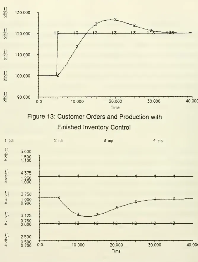
Figure 13

shows

a simulation of the finished inventory monitoring

and

control policy, with a

20

percent increase in sales effort.

The

reader

1] 2 11 2 3J 2 3J 1) 2 3 3) 130.000 120,000 110 000 100.000 90 000 H I

—

I I '

—

I

—

I

—

'

—

I >

—

I—'

—

' ' ' I

—

''-I

—

' I

''''

I • • 1 0.0 10.000 20.000 30.000 40 000 Time

Figure 13:

Customer

Orders

and

Production with

Finished Inventory Control

1 pdi i) 3 4 i] 3 4 I] 3 4

2 idi 3 aqi 4 eis

41 4 5.000 1.500 1.100 4.375 1 250 1.000 3.750 1 000 0.900 3.125 750 0.800 2500 500 . 0.700 00 -Hj--\

—

'—'

—

'

—

I •~ 10.000 -4-^2 1-3 i^

«

1^ 1-3-20.000 Time — 1 1 1 1 1 1 . r— 30.000 40.000

D-3807

29

increases,

customer

orders (-1-) increase correspondingly to 120 units

per month.

Now

tnowever, orders (-1-) remain constant rather than

declining. Meanwhile, production (-2-) increases slowly until it equals

customer

orders in

month

12. Production (-2-) continues to grow,

peaks

at about 125 units per

month

then gradually declines until it balances exactly

with orders.

The

production overshoot enables the factory to re-build its

depleted finished inventory back to 3

months

worth of shipments.

Figure 14

shows

that the

new

policy holds delivery interval (-1-) rock

steady at 3

months

--

_because

_{there is}

_adequate

_{inventory on}

_hand

_to

prepare

and

ship all

customer

order in three

months,

despite the unexpected surge of orders. In other

words

the finished inventory acts as a

buffer to insulate

shipments

from production. Figure 15

shows

how

inventory also acts as a source of planning information for production planners. In

month

5

(when customer

orders step-up) inventory (-1-)

declines,

because

shipments

exceed

production. At the

same

time

authorized inventory (-2-) begins to rise,

because

shipments

are

now

higher

and

the factory

needs

more

finished inventory in order to maintain

3

months

coverage

of shipments.

The

difference

between

authorized

inventory (-2-)

and

actual inventory (-1-) is the signal that planners use to increase the production plan

-

it's the analogy of excess orders in the

order control policy. Planners

add

half the inventory discrepancy to the

six-month forecast in order to

compute

planned production six-months ahead.

The

simulation

shows

that the planners' correction to the forecast

(-4-) rises to a

peak

of

20

units per

month

by

month

12, declines to zero

by

month 27 and goes

slightly negative

between

months 28 and

40. With

the inventory control policy in effect, planners

expand

the production

schedule

more

quickly than the forecast alone

would

suggest -- _{just as}

they did with the order control policy. Figure 16

shows

what

is happening.

As

before, the short-term business forecast (-1-) rises slowly from

100

to

120

units per month. In

month

10, forecasters are predicting that

customer

orders will be

110

units per

month

in six

months

time. But in

month

10, planners are preparing to produce 125 units per

month

(-2-) by

month

16.

They

justify the extra planned production on the basis of the

finished inventory shortfall. In fact, the shortfall tells

them

to plan

above

forecast all the

way

from

month

5 to

month

25

of the simulation.

The

D-3807

31

1 n 2 ai 3 cpi 4 cpoi

1

DOCUMENTATION OF THE

SALES

AND

PRODUCTION

SCHEDUUNG MODELS

Policy Structure of the Sales

and

Production Scheduling

Model

STELLA

Diagram

of

Customer

Ordering

and

Forecasting in the

Base

Sales

and

Production Scheduling Model (saps_base)

STELLA

Diagram

of Delivery Interval in the

Base

Sales and Production Scheduling Model (saps_base)

STELLA

Diagram of Production Scheduling

and

Expediting in the

Base

Sales

and

Production Scheduling Model (saps_base)

STELLA

Equations forthe

Base

Sales

and

Production Scheduling Model (saps_base)

STELLA

Diagram of Order Monitoring, Production Scheduling

and

Expediting

in the Sales

and

Production Scheduling

Model

with

Order Monitoring

and

Control (saps_ordmon)

STELLA

Equations for the Sales and Production Scheduling Model with

Order Monitoring

and

Control (saps_ordmon)

STELLA

Diagram of

Customer

Ordering

and

Forecasting in the

Sales

and

Production Scheduling Model

with Finished Inventory Control (sapsjnvcon)

STELLA

Diagram

of Finished Inventory Control

and

Shipping in the

Sales

and

Production Scheduling Model

D-3807

33

DOCUMENTTATION

OF

THE SALES

AND

PRODUCTION SCHEDULING

MODELS

-

_CONTINUED

STELLA

Diagram

of Delivery Interval in the

Sales and Production Scheduling Model

with Finished Inventory Control (sapsjnvcon)

STELLA

Diagram of Order Monitoring, Production Scheduling

and

Expediting

in the Sales and Production Scheduling Model with Finished Inventory Control (sapsjnvcon)

STELLA

Equations forthe Sales

and

Production Scheduling Model

with Finished Inventory Control (sapsjnvcon)

Description of

New

Structure

and

Equations to Convert

- .::::: Monufocturinq ; ;Production :::::::::::::::: irrrrrrT::::::: P'onninq _::;;:: ':::::::::::::::::::::::::::: _Horizon ••••• EXPEDITING ::::::::::::::: :::::: Ai-ilite R

Figure17: Policy Structure of the Sales

and

D-3807

35

Figure 18:

STELLA

Diagram

of

Customer

Ordering

and

Forecasting in the

Base

Sales

and

Production Scheduling Model (saps_base)

\r\rrr\ pVannt A orderi

Figure 19:

STELLA

Diagram

of Delivery Interval in the

D-3807

37

Figure 20:

STELLA

Diagram of Production Scheduling

and

Expediting in

INIT(fpo) = stbf»mph 0.0 -> 0.800

Ob = Ob + CO - s 0.500 -> 0.850

INIT(ob) = 300 1.000 -> 1.000

n

pdi = pdi cpdi 1.500 -> 1.150

INIT(pd1) = idi 2.000 -> 1.350

D

stbf = stbf + cstbf 2.500 -> 1.550 INIT(stbf) = CO 3.000 -> 1.825 aporstbf 3.500 -> 2.150

O

CO = se/ts 4.000 -> _2.500

O

cpdl = (edi-pd1)/tpdi 4.500 -> _2.900

O

cse = .2 5.000 -> 3.500 cstbf = (co-stbf)/taf

O

d1 = ob/p

O

edi = (ob/fpo)*mph

O

fp = .3

O

fpoc = ob/fpo

O

idi = 3

O

ise = 7500 niph = 6 nts = 75 P = ss*fp+psp*(1 -f_p)

O

powil = fpo*(id1/mph) psp = fpo/mph rco = se/nts

O

rdi = pdi/idi s _{= p}

se = IF TIME <5 THEN ise ELSE (ise»(1+cse))

O

ss = ob/pdi

C

taf = 6

O

tpdi = 1

ts = nts*edits

STELLA

Equations for the

Base

Sales

and

Production Scheduling Model (saps_base)

D-3807

39

Figure 21:

STELLA

Diagram

of Order Monitoring, Production Scheduling

and

Expediting in the Sales

and

Production Scheduling

Model

with Order Monitoring

and

Control (saps_ordmon)

fpo = fpo p + apo INIT(fpo) = stbf»mph lj Ob = ob + CO - _s INIT(ob) = 300 Lj pdl = pdi + cpdi INIT(pdl) = idi stbf = stbf + cstbf INIT(stbf) = CO apo = stbf+(uo/tcuo) CO = se/ts

O

cpdi = (edi-pd1)/tpdi cse = .2 cstbf = (co-stbf)/taf

O

cwos =

O

di = ob/p

O

edi = (ob/fpo)*mph

O

fp= 3

O

fpoc = ob/fpo

O

idi = 3

J

ise = 7500

O

iwos = "j _{mph = 6}

O

nts = 75

C

OS = fpo*fpoc

O

p = ss*fp+psp*(l-fp)

O

powii = fpo*(idi/mph) C-' powti = fpo*(pd1/mph)*(1-wft)+fpo*(idi/mph)*wft

C

psp = fpo/mph

O

rco = se/nts

O

rdi = pdi /idi

rpo = os*wos+powti*(1-wos)

1 s = _p

STELLA

Equations for the Sales

and

Production Scheduling Model

D-3807

41

se = IF TINE <5 THEN ise ELSE (ise*(1*cse))

Q

ss = ob/pdi

O

taf = 6

O

tcuo = 1

O

tpdi = 1 ts = nts*edits

O

uo = ob-rpo

O

wft = 1

O

wos = IF TIME < 40 THEN iwos ELSE (iwos*(1+cwos))

edits = graph(rdi) 0.0 -> 0.800 0.500 -> 0.850 1.000 -> 1.000 1.500 -> 1.150 2.000 -> 1.350 2.500 -> 1.550 3.000 -> 1.825 3.500 -> 2.150 4.000 -> 2.500 4.500 -> 2.900 5.000 -> 3.500

STELLA

Equations Continued -- _{for the Sales}

_and

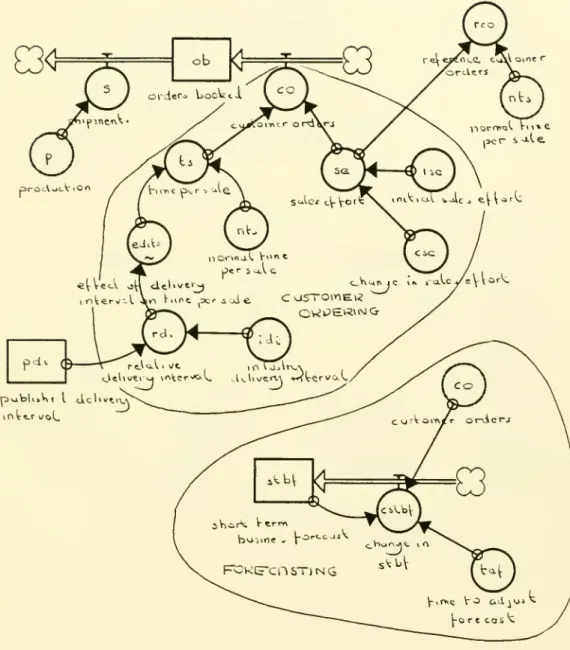
_Production

Figure 22:

STELLA

Diagram of

Customer

Ordering

and

Forecasting

in the Sales

and

Production Scheduling

Model

with Finished Inventory Control (sapsjnvcon)

D-3807

43

Figure 23:

STELLA

Diagram

of Finished Inventory Control

and

Shipping

in the Sales

and

Production Scheduling

Model

Figure 24:

STELLA

Diagram

of Delivery Interval in the

Sales

and

Production Scheduling

Model

D-3807

45

INIT(asl) = si

Hj fi = fi + p - si

INIT(fi) = co*8ic

Cj fpo = fpo + apo

-p

INIT(fpo) = stbf*mph ob = Ob + CO - _s INIT(ob) = 300

Lj pdi = pdi + cpdi

INIT(pdi) = idi

n

slbf = stbf + cstbf INIT(stbf) = CO

O

9i = asi*aic

O

aic = 3 apo = stbf+(uo/tcuo)+(cpoi*wic)

O

aqi = fi/(ss*aic)

O

casi = (si-asi)/tas

O

CO = se/ts

O

cpdi = (edi-pdi)/tpdi

O

cpi = (ai-fi)/tcip

O

cpoi = (ai-fi)/tcis cse = .2

C

cstbf = (co-stbf)/taf ''_ _{cwos =} di = ob/si

O

edi = (ob/fpo)*mph*(1-wdi)+di*wdi

C

fp = -3 ;~; _{fpOC = Ob/fpO}

C

idi = 3

O

ise = 7500 iwos = 1

O

mph = 6

O

nts = 75 ~; OS = fpo*fpoc

STELLA

Equations forthe Sales

and

Production Scheduling Model

1^ I

D-3807

47

O

p = (ss+cpi)*fp+psp*(1-fp) powii = fpo*(icli/mph) powti = fpo*(pdi/mph)*(1-wft)+fpo*{id1/mph)*wft

O

psp = fpo/mph

O

rco = se/nts rdi = pdi/idi

O

rpo = os*wos+powti*(1-wos) '.0 s = si

se = IF TIME <5 THEN ise ELSE (ise*(l+cse))

si = ss*eis ss = ob/pdl

C

taf = 6

C

tas= 12

O

tcip = 2 tcis = 2 tcuo = 1

O

tpdi = 1

O

ts = nts*edits I

J

uo = ob-rpo C' wdl = 1 wft = wic = 1

wos = IF TIME < 40 THEN iwos ELSE (1wos*(1*cwos))

edits = graph(rdi)

!

eis = graph(aqi)

0.0 -> _0.800 0.0 -> 0.0 0.500 -> 0.850 0.200 -> 0.950 1 000-> 1.000 0.400 -> 0.980 1.500 -> 1.150 0.600 -> 1.000 2.000 -> 1.350 0.800 -> 1.000 2.500 -> 1.550 1.000 -> 1.000 3.000 -> 1.825 1.200 -> 1.000 3.500 -> 2.150 1.400 -> 1.000 4.000 -> 2.500 1.600 -> 1.000 4 500 -> 2.900 1.800 -> 1.000 5.000 -> 3.500 2.000 -> 1.000

STELLA

Equations Continued -- _{for the Sales}

_and

_Production

DEFINITION

OF

VARIABLE

NAMES

ai authorized inventory (systems)

aic authorized inventory coverage (months)

apo additions to planned orders (systems/month)

asi average shipments from inventory (systems/month)

aqi

adequacy

of inventory (dimensionless)

casi

change

in average shipments from inventory

(systems/month/month)

CO

customer

orders (orders for systems/month)

cpdi

change

in perceived delivery interval (months/month)

cpi correction to production from inventory (systems/month)

cpoi correction to planned orders from inventory (systems/month)

cse

change

in sales effort (dimensionless)

cstbf

change

in short-term business forecast

(systems/month/month)

cwos

change

in weight for orders scheduled (dimensionless)

di delivery interval (months)

edi estimated delivery interval (months)

edits effect of delivery interval on time per sale (dimensionless)

eis effect of inventory on shipments (dimensionless)

fi finished inventory (systems)

fp flexibility of production (dimensionless)

fpo firm planned orders (systems planned)

fpoc fraction of planned orders committed (dimensionless)

id! industry delivery interval (months)

ise initial sales effort (hours/month)

iwos initial weight for orders scheduled (dimensionless)

mph

manufacturing planning horizon (months)

nts normal time per sale (hours/system)

ob orders

booked

(orders for systems)

OS orders scheduled (systems planned)

p production (systems/month)

pdi published delivery interval (months)

D-3807

49

DEFINITION

OF

VARIABLE

NAMES

-

_CONTINUED

powti planned orders within target interval (systems planned) psp production suggested by plan (systems/month)

rco reference

customer

orders (orders for systems/month)

rdi relative delivery interval (dimensionless)

rpo reference planned orders (systems planned)

s shipments (systems/month)

se sales effort (hours/month)

si shipments from inventory (systems/month)

ss scheduled shipments (systems/month)

stbf short-term business forecast (systems/month)

tat time to adjust forecast (months)

tas time to average shipments (months)

tcip time to correct inventory for production (months)

tcis time to correct inventory for schedule (months)

tcuo time to correct unexpected orders (months)

tpdi time to publish delivery interval (months)

ts time per sale (hours/system)

uo unexpected orders (orders for systems) wdi weight for delivery interval (dimensionless)

wft weight for fixed target (dimensionless)

wic weight for inventory correction (dimensionless)

DESCRIPTION

OF PARAMETER

AND

STRUCTURAL

CHANGES

FOR

SIMULATION

SCENARIOS

Base

Run

(Model saps_base)

The

base

run is described on

pages

15 through 19 of the report.

The

base

run uses the

model saps_base

-- _{a version of the}

_model

_{in which there is}

no feedback to production planning from orders booked,

and

in which there

is no finished inventory.

The

production plan (more specifically, additions

to

planned

orders) is therefore equal to the forecast.

The

forecast is

assumed

to

be

an exponential

smoothing

of

customer

orders, with a smoothing constant (time to adjust the forecast taf) of 6 months.

Monitoring

and

Control of Excess Orders (model

saps_ordmon)

The

model

saps_ordmon

is the

same

as the

base

model, but with

new

equations to represent a policy of monitoring

and

control of excess orders.

Simulations of the

model

are described on

pages 20

through

24

of the

report.

The

new

equations are described below.

a). Additions to Planned Orders

apo

= stbf + uo/tcuo 1

tcuo = 1 2

where:

apo

additions to planned orders (systems planned/month) stbf short-term business forecast (systems/month)

uo unexpected orders (orders for systems)

D-3807

51

In the

base

model, the additions to planned orders (apo) are equal to the

short-term business forecast (stbf). In other words,

when

planners

add

new

production orders to the production schedule, they

add

the

number

of

orders called for by the forecast (stbf). But,

when

they adopt the order monitoring

and

control policy they also

add

a proportion of the unexpected

orders (uo) on top of the forecast.

When

the forecast is innaccurate, or

more

specifically,

when

it is biased

downward,

unexpected

orders

accummulate

which are factored into the production plan as

shown

in

equation 1

.

b). Unexpected Orders

But

what

are unexpected orders

and

how

do

schedulers recognize

them?

Equations 3 through 9

show

how.

where:

uo = ob - rpo

rpo =

os*wos

+ powti*(1-wos)

OS = fpo*fpoc fpoc = ob/fpo

wos

weight for orders scheduled (dimensionless)

powti planned orders within target interval (systems)

pdi published delivery interval (months)

idi industry delivery interval (months)

mph

manufacturing planning horizon (months)

wft weight for fixed target (dimensionless)

The

equations contain two switches -- _{weight for orders scheduled (wos)}

and

weight for fixed target (wft)

which

allow

one

to

make

different

assumptions

about the effectiveness of the order monitoring

and

control

policy.

The

simulations described in the report

were

obtained by setting

wos

=

and

wft = 1 -- a combination of switches that results in very

effective order monitoring

and

control. With this combination, the

equation for reference planned orders (rpo) reduces to:

rpo = fpo*(idi/mph)

So,

we

are saying in equation 3 that schedulers recognize

unexpected

orders (uo) by comparing orders

booked

(ob) with reference planned orders

(rpo),

and

that they take as their reference point only the planned orders

scheduled

for production within the industry's delivery interval (the

quantity fpo*(idi/mph).

If the parameter, weight for orders scheduled (wos), is set to 1, then the

model

saps_ordmon

becomes

equivalent to the

base

model.

Under

this

condition, the equation for reference planned orders (rpo) reduces to:

rpo = OS

But, as equations 5

and

6 show, orders scheduled (os) are those planned

orders that

have been

assigned to

customer

orders -- _{in other words,}

D-3807

53

and

in equation 1 additions to planned orders (apo) are equal to the

short-term business forecast (stbf) -- _the

same

_assumption

_used

_{in the}

base

model.

(One

might ask,

why

take the trouble to write equations for

reference planned orders (rpo) if the numerical value of reference planned

orders (rpo) is zero.

The

answer

is that the equations

show

the process by

which schedulers

and

planners recognize excess orders -- _{the information}

they use to assess whether customers have ordered

more

than expected. It

turns out that in a

system

where

schedulers

have

the

freedom

to assign

customer

orders to

any

open

production slot (a slot-planning system) it's

difficult to recognize

excess

orders because, if the planning horizon is

long enough, schedulers can always find

open

production slots).

Finished Inventory Control (model

sapsjnvcon)

The

model

sapsjnvcon

is the

same

as

saps_ordmon,

but with equations

added

to represent finished inventory, production for inventory, shipping

from inventory (in

saps_ordmon

shipping is equal to production)

and

finished inventory control.

The

new

equations are described below.

a). Finished Inventory

and

Shipping

ufi = fi + p - si 1

INIT(fi) = co*aic 2

si = ss*eis 3

eis = graph(aqi)

4

where:

fi finished inventory (systems)

p production (systems/month)

si shipments from inventory (systems/month) CO customer orders (orders for systems/month)

aic authorized inventory coverage (months) ss scheduled shipments (systems/month)

eis effect of inventory on shipments (dimensionless)

aqi

adequacy

of inventory (dimensionless)

Equation 1 states that finished inventory (fi) is increased by production

(p)

and reduced

by

shipments

from inventory (si).

So

production

and

shipments are no longer identical as they

were

in the

base

model and

in

saps_ordmon,

but can

move

(somewhat)

independently

because

they are

separated by a level of inventory.

Equations 3 through 5 describe shipping. If there is

adequate

finished

inventory then

shipments

from inventory (si) are equal to the shipping

schedule (ss).

The

factory can ship according to schedule

because

there is

adequate

product available -- _{in other words, the effect of inventory on}

shipments (eis) is neutral (takes a numerical value of 1).

The

key to the

success

of the finished inventory control policy is for the factory to hold

enough

finished inventory that stockouts of high-volume items never

occur.

By

preventing stockouts, the factory can maintain constant delivery intervals

and

so avoid the possibility of inadvertently suppressing

customer

orders.

The

following parameter values represent a no-stockout

D-3807

55

authorized inventory coverage aic = 3

months

effect of inventory on shipments eis = graph(aqi) such that

when

adequacy

of inventory

aqi = eis = aqi = 0.2 eis = .95 aqi = 0.4 eis = .98 aqi = 0.6 eis

=1.0

aqi = 0.8 eis = 1.0 aqi = 1.0 eis = 1.0 aqi = 1.2 eis = 1.0 aqi = 1.4 eis = 1.0 aqi = 1.6 eis = 1.0 aqi = 1.8 eis = 1.0 aqi = 2.0 eis

=1.0

It is important that the effect of inventory on shipments (eis) remains at

the value 1, or very close to 1, over a wide range of values of finished inventory,

because

then the factory is always able to ship acording to

schedule. If you study the graph function for the effect of inventory on

shipments

you'll

see

that

when

adequacy

of inventory is 1 --

when

the

factory's finished inventory is exactly equal to the authorized inventory,

which is three

months

of

shipments

-- _{then the effect of inventory on}

shipments (eis) is also 1.

When

the

adequacy

of inventory (aqi) falls

--when

the factory's inventory is less than authorized -- _{the effect of}

inventory on shipments (eis) stays very close to the value 1 . Only

when

the

adequacy

of inventory reaches the value .2 --

when

_{the factory's is only}

one

fifth of the authorized --

_does

_{the effect of inventory on shipments}

some

product lines

and

therefore unable to ship according to schedule.

The

reader should be

aware

that

one

cannot arbitrarily specify the

shape

of the effect of inventory on shipments (eis).

The

shape

depends

on the

authorized inventory

coverage

(aic)

and

on the diversity of products the factory produces

and

holds in finished inventory. If the factory produces

many

different products then it should plan to hold a lot of finished inventory (in other words, the authorized inventory coverage will be high,

say 3 or 4

months

of shipments) to be sure of avoiding stock-outs,

and

therefore to be sure that the effect of inventory

on

shipments remains

close to the value 1.

On

the other hand, if the factory produces only

one

product line, a stock-out can occur only

when

finished inventory is zero.

So

the effect of inventory on shipments (eis) will remain at the value 1

even

if the factory's authorized inventory coverage (aic) is only

one month

or

one

week

of shipments.

So,

when

using the

model

sapsjnvcon,

it is important to think carefully

about the

shape

of the effect of inventory on shipments (eis)

- how

it

changes

depending on the factory's authorized inventory coverage (aic) and

on the assumptions

one

makes

about the factory's

number

of product lines.

For example, if

one were

to rerun

sapsjnvcon

with authorized inventory

coverage reduced

to only

one

month, instead of three, (and with the

assumption

that the factory

produces

several, say 10, different product

D-3807

57

shipments (eis) slope

more

gradually

upward

from the (0,0) point.

One

would

find that, the

more

gradual the slope, the less effective the

inventory control policy

would

be in regulating delivery interval

--because

the factory would stock-out

more

easily.

b). Finished Inventory Monitoring

and

Control

To

use

the finished inventory effectively for production planning, the

factory's

warehouse

must

monitor the difference

between

finished

inventory

and

authorized inventory

and

report the difference to schedulers

and

planners.

The

schedulers

and

planners use the information to adjust both current production

and

the production plan.

The

equations to represent

the monitoring

and

control of finished inventory are

shown

below:

apo

= stbf + (uo/tcuo) + (cpoi*wic) 6

cpoi = (ai - _fi)/tcis 7

p = (ss + cpi)*fp + psp*(1-fp) 8

cpi = (ai - fi)/tcip 9

where:

apo

additions to planned orders (systems/month) stbf short-term business forecast (systems/month) uo unexpected orders (orders for systems)

tcuo time to correct unexpected orders (months)

cpoi correction to planned orders from inventory

(systems/month)

ai authorized inventory (systems)

fi finished inventory (systems)

tcis time to correct inventory for scheduling (months) p production (systems/month)

cpi correction to production from inventory

(systems/month)

fp flexibility of production (dimensionless)

psp production suggested by plan (systems/month)

tcip time to correct inventory for production (months)

Equation 6 states that

when

planners

make

additions to planned orders they

add

to the short-term busines forecast (stbf) a correction to planned

orders from finished inventory (cpoi).

They

make

a correction

whenever

there is a reported difference

between

authorized inventory (ai)

and

finished inventory (fi) as

shown

in equation 7. (They also

add

to the

short-term business forecast (stbf) a correction for

unexpected

orders

(uo)

-

but in the simulations

shown

in the report,

unexpected

orders are

always zero

because

reference planned orders (rpo) are equal to orders scheduled (os)).

Equation 8

and

9 state that schedulers

make

a correction to production

(cpi)

based

on the reported difference

between

authorized inventory (ai)

and

finished inventory (fi). If finished inventory (fi) is lower than

authorized (ai) they

add a

portion of the difference to scheduled shipments in order to

consume

the schedule of planned orders

more

quickly

and

so