Congestion Control in the context of Machine Type Communications in Long Term Evolution networks

(1)

HAL Id: dumas-00636132

https://dumas.ccsd.cnrs.fr/dumas-00636132

Submitted on 26 Oct 2011

HAL is a multi-disciplinary open access

archive for the deposit and dissemination of sci-entific research documents, whether they are pub-lished or not. The documents may come from teaching and research institutions in France or abroad, or from public or private research centers.

L’archive ouverte pluridisciplinaire HAL, est destinée au dépôt et à la diffusion de documents scientifiques de niveau recherche, publiés ou non, émanant des établissements d’enseignement et de recherche français ou étrangers, des laboratoires publics ou privés.

Congestion Control in the context of Machine Type

Communications in Long Term Evolution networks

Ahmed Amokrane

To cite this version:

Ahmed Amokrane. Congestion Control in the context of Machine Type Communications in Long Term Evolution networks. Networking and Internet Architecture [cs.NI]. 2011. �dumas-00636132�

(2)

ENS Cachan, Britanny extension University of Rennes I

Research Master in Computer Science, Networks and Distributed Systems

Master thesis internship report

Congestion Control in the context of Machine Type

Communications in Long Term Evolution networks

Work done by : Ahmed Amokrane ahmed.amokrane@ens-cachan.fr Supervisors: Adlen Ksentini adlen.ksentini@irisa.fr Yassine Hadjadj-Aoul yassine.hadjadj-aoul@irisa.fr Dionysos team

Irisa / Inria Rennes Bretagne Atlantique

(3)

Abstract

Machine Type Communications (MTC) are automated applications which involve machines or devices that communicate through a network without any human intervention. They can be used today in almost everyday life applications from military to civil applications, such as: transportation, health care, smart energy, supply and provisioning, city automation... Those devices are generally spread in a wide area and should communicate through widely deployed networks. A good candidate to play the role of such a network could be cellular mobile networks. In fact, Cellular networks have been already deployed and offer a large coverage. Such a deployment is beneficial for both mobile network Operators (i.e. more revenues) and the application developers (i.e. more opportunities). Furthermore, LTE networks are all-IP networks and offer a good support for MTC. However, cellular networks are not designed for MTC applications. Consequently, such a deployment is challenging and rises new problems. The most important of them is congestion. In fact, in MTC, a huge number of devices are deployed. This leads to contention and congestion in the the different parts and nodes of the network when a lot of devices communicate at the same time. In the present work, we propose a novel Congestion-Aware Admission Control solution, which deals with the congestion in LTE networks. Our solution, which is based on control theory, effectively allows avoiding the core network congestion while saving the wireless scarce resources. We show its effectiveness through network simulations carried on the ns-3 simulator. In fact, the obtained results show that our solution is robust against different traffic patterns and accommodates huge amount of devices as expected in this particular case of MTC applications. It assures a targeted utilization of the resources in the network. Furthermore, it is completely compliant with the actual protocols and standards.

(4)

List of Figures

1 A general architecture of a M2M application . . . 6

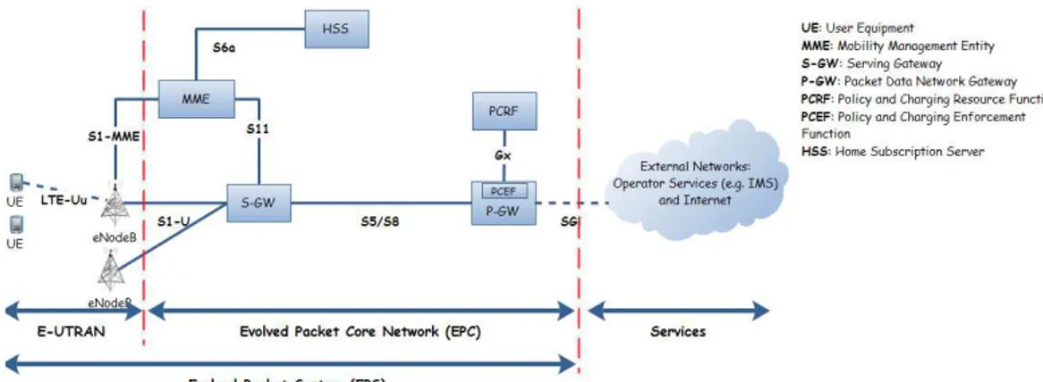
2 The LTE Global architecture . . . 7

3 Sequence Diagram for signaling and data in case of Event Driven and Time Driven

applications . . . 9

4 Sequence Diagram for signaling and data in case of Query Driven applications . . . 9

5 PID controller, general diagram . . . 10

6 The impact of the gains (Kp, Ki and Kd) on the output value [1] . . . 11

7 The congestion problem in LTE network in the context of MTC applications . . . 12

8 LTE Network Architecture . . . 15

9 General Overview of the Solution . . . 18

10 LTE Network Testing Topology . . . 21

11 The Signaling traffic generated by the MTC Devices in case of bursty traffic . . . . 22

12 The Reject Factor evolution in the MME and the Reject Probabilities in the

dif-ferent eNodeBs in case of Bursty traffic . . . 23

13 The Reject Factor evolution depending on the signaling traffic received and the

queue length in the MME in case of Bursty traffic . . . 23

14 Comparison between the case where a PID queue and drop tail queue are used in

the MME in the case of Bursty traffic . . . 24

15 The Signaling traffic generated by the MTC Devices in case of Uniform traffic . . . 25

dif-ferent eNodeBs in case of Bursty traffic . . . 26

queue length in the MME in case of Uniform traffic . . . 26

the MME in case of Uniform traffic . . . 27

19 The Signaling traffic generated by the MTC Devices in case of Uniform traffic with

bursts . . . 28

dif-ferent eNodeBs in case of Uniform traffic with bursts . . . 29

queue length in the MME in case of Uniform traffic with bursts . . . 29

the MME in case of Uniform traffic with bursts . . . 30

23 The Signaling traffic generated by the MTC Devices in case of Random traffic . . . 31

dif-ferent eNodeBs in case of Uniform traffic with bursts . . . 32

queue length in the MME in case of Random traffic . . . 32

(6)

1 Introduction

Machine Type Communications (MTC) (also called Machine-to-Machine (M2M)) are automated applications which involve machines or devices communication through a network without any human intervention. They can be used today in almost all everyday life applications from military to civil applications, such as: transportation, health care, smart energy, supply and provisioning, city automation, and manufacturing. The communicating devices can be embedded in different environments like cars, cell towers, vending machines...etc. They are generally spread in a wide area and should communicate through widely deployed networks. A good candidate to play the role of such networks could be the cellular mobile networks.

Cellular mobile networks offer different network technologies for M2M communications. There are strong realistic predictions stating that M2M will be leveraged over cellular mobile networks. In fact, such integration represent many advantages for both Mobile Network Operators (MNO) and application developers. It will provide MNO with more revenues and the applications devel-opers with more opportunities. Therefore, efforts are being conducted to enable such deployment.

The 3rd Generation Partnership Project (3GPP)1

[2] is working on specifications to standardize the deployment of M2M applications in 3GPP networks (UMTS and LTE). However it is chal-lenging and not trivial. In fact, cellular networks (among them LTE) are designed for Human-to-Human (H2H), Human-to-Machine (H2M) and Machine-Human-to-Human (M2H) applications, which are different from M2M. Thus, MNO should accommodate their networks to support the M2M applications which involve a huge amount of autonomous devices. One of the most important problems posed by that deployment is congestion. Congestion concerns all the parts of the net-work, both the radio and the Core Network. It is due, mainly, to the fact that MTC devices are deployed in a huge number and are generally synchronized (more likely to send data at the same time). This may lead to peak load situations and may have a tremendous impact on the operations of the mobile network, penalizing both MTC and non-MTC devices. For instance, if many devices detect an event at the same time, they send their alerts toward a central server at the same time, leading to congestion in the different nodes of the network.

In the present work, we propose a novel solution to handle the congestion in LTE networks in the particular context of MTC applications. Our solution is implemented at the network level (IP) and doesn’t impose any constraint on the applications. It combines the actions of both a Congestion Control and an Admission Control: it uses an queue monitoring based on a Proportional, Derivative and Integrative (PID) controller implemented in each Core Network node to detect congestion while enabling Admission Control which rejects traffic in the radio part. Practically, the core network nodes monitor congestion and define the parameters of the Admission Control in the radio part.

Furthermore, we give some numerical results on the simulations performed under the ns-3 [3] simulator. The results concern the context of MTC applications through traffic load and patterns that are more likely to be those of MTC. We show the effectiveness of our proposal through the obtained results. In fact, we succeeded to reduce the amount of signaling, to reach a targeted

1

3GPP is a collaboration between groups of telecommunications associations that aim to standardize the 3G and the 4G Mobile systems to come through LTE and LTE advanced. It is composed of European Telecommunica-tions Standards Institute (ETSI), Association of Radio Industries and Businesses/Telecommunication Technology Committee (ARIB/TTC, Japan), China Communications Standards Association (CCSA), Alliance for Telecom-munications Industry Solutions (ATIS, North America) and TelecomTelecom-munications Technology Association (TTA, South Korea).

(7)

utilization of resources in the core network part and to avoid losses (overflow in the queues). Note that our proposal is completely compliant with the existing standards and existing architectures. The remainder of this document is organized as follows. First, Section 2 presents a gentle overview of M2M, LTE networks and PID controllers. The problem of congestion as well as the related works are, also, presented in this section. Section 3 presents a general and detailed description of our proposed solution. The proposed solution is, then, evaluated in Section 4 through simulations and discussions on the results. Then, Section 5 discusses our proposed solution. Finally, Section 6 concludes the document.

2 Background and related works

In this section, we briefly present some generalities on MTC, LTE networks and the Proportional, Integrative and Derivative (PID) controller we are using. Then the congestion problem we are tackling is presented as well as the related works in literature.

2.1 Overview of Machine Type Communications

MTC or M2M is, usually, a form of data communication which involves one or more entities that do not necessarily need human intervention [4]. In a practical scenario, a common M2M application uses a device (sensor, meter...) to capture an event (temperature, inventory level, etc.) by converting analog measurements to digital data, more precisely IP packets. The digital data is sent through a network (wireless, wired or hybrid, UMTS, LTE..., depending mainly on the

required QoS [5] and the cost) to an application (software program) called a server2

. The latter translates it into meaningful information (data stored, threats detected...) [6, 7]. Afterwards, answers could be sent back to the devices.

The devices involved in a M2M application and having the required functionalities, consisting in replaying to requests and/or sending data by themselves, are called M2M devices (or MTC devices) [4].

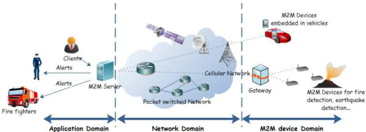
A generic and simple architecture of a MTC application is illustrated in Figure 1. The architecture is mainly composed of mainly three parts: M2M Device Domain containing the MTC devices, Network Domain which transports the messages between the MTC devices and the servers located in the Application Domain, giving data to business applications the devices are deployed to. The network domain could be UMTS or LTE as we will see it in details later.

MTC applications are different from H2H, M2H and H2M applications. In fact, they should behave and assume their roles without any human intervention. Furthermore, they are char-acterized by some properties that make them a bit more different. The main properties are [4]:

• Large number of devices: Typical applications require a lot of devices deployed in the same area leading to high density or distant leading to a large spread.

• Devices can send and/or receive frequently or infrequently small amounts of data (low data rates).

2

(8)

Figure 1: A general architecture of a M2M application

• Low mobility for devices meaning that they don’t move, move infrequently or move in a predefined region.

• Reduced costs as these applications are used in everyday life and may involve a large number of devices.

• Devices may be grouped into Groups. This is interesting for charging, policing and multicast (toward a group).

• Devices should require ultra low power consumption.

• Time tolerant (generally), since data can be usually delayed. However, real-time transmis-sion should also be considered for some applications.

• Time controlled as the devices may send and receive data only at certain periods of time. • Security of exchanges between the devices and the server.

2.2 MTC applications taxonomy

It is worth to start by making things clear. MTC applications as they are thought in the context of sensors and servers (the typical cases we introduced in the previous paragraph), should be classified to make their study easier. We propose the classification of MTC applications into three main classes. Note that this is our classification we propose in the context of MTC. It comes from the data reporting way in Wireless Sensor Networks [8]. The criterion upon which we classify them is the traffic (signaling and data) and its origin. Note that a fourth class combining the three previous ones can exist.

1. Event Driven applications: The MTC devices send messages when an event occurs in the sensed area. For instance, messages are send when an intrusion is detected in a common application of security. Generally, this is considered to have more priority than the rest of the applications. However, the amount of data they send is small since the message to signal the event is generally short.

(9)

Figure 2: The LTE Global architecture

2. Query Driven applications: This is a common interactive application. Generally, the client sends a query to the server (see the temperature in the office). The server then sends the query to the sensor responsible to monitor the area concerned by the query (The sensor inside the office). The answer is then given by the MTC-Device. Note that the actuators are query driven applications since they behave in the same manner, i.e: they act according to the orders coming from the server.

3. Time Driven applications: The MTC-Devices send their messages (reports, sensed val-ues...) to the server at regular rates (each hour for instance). The server is generally responsible for the rest of the treatment concerning the data.

2.3 Overview of the Long Term Evolution (LTE) networks

The LTE networks are the next generation of the deployed 3GPP networks. Their main target is a simplified architecture in comparison to its predecessors (UMTS) and the rates of 50 Mbps in uplink and 100 Mbps in downlink. They are under heavy standardization efforts led by 3GPP.

The global architecture of an LTE network is illustrated in Figure 2. It is composed of two main parts: the E-UTRAN (Evolved UMTS Terrestrial Radio Access Network) and a EPC (Evolved Packet Core Network). Furthermore, LTE networks are all-IP networks. This means that all the traffic that is transported in the network is IP packets. Moreovere, traffic is divided into signaling and data. Signaling is the messages a UE (User Equipment) sends to connect to the network and data is the useful messages that the UE send. For instance, in a voice call, the signaling is the messages sent by the UE to connect to the network and ask for the call, while, the data is the voice call when connexion is established.

1. E-UTRAN part: It is composed of the UEs and the eNodeB. eNodeB are the Base Stations that integrate functionalities like radio management.

2. EPC part: It is the Core Network part in the LTE network. It is responsible for the overall control of the UE and the establishment of bearers between the UE and the PDN Gateways (For simplicity, a bearer is a packet flow or tunnel between a UE and the P-GW. It is IP-only network. It comprises five logical nodes :

(10)

• Packet Data Network Gateway (P-GW): It insures the connexion with the IP Network of the operator. It is responsible for allocating IP addresses for UEs. It, also, filters downlink packets into bearers of different QoS and destinations (UEs). Furthermore, it is the anchor point for internetworking with non-3GPP networks such as CDMA2000 and WiMAX.

• Serving Gateway (S-GW): It serves as an anchor for data bearers when UE moves from eNodeB to another (handover). It also holds data of downlink bearers when UE is in idle state (turned off to save power, to release the radio bandwidth it uses for others...) and while the MME re-establishes the bearer with the UE. Similarly with P-GW, it serves also as an anchor, but this time, for internetworking with 3GPP networks (UMTS, GPRS...).

• Mobility Management Entity (MME): It is a key element in the LTE architecture as it is responsible for processing signaling between UE and the Core Network. It assumes functions related to both bearer management (establishment, maintenance and release) and functions related to attachment and connection management (establishment of the connection and security between the network and UE, authentication). It helps, as well, to reduce the overhead in the radio network by holding informations about UEs, which ensures a continuity when the UEs are in idle sates. These functions are handled by the Session Management Layer in the Non-Access Stratum (NAS) protocol [9]

• The Policy Control and Charging Rules Function (PCRF): It is responsible of the policy control decision making and the management of the flow based charging functionalities in the Policy Control Enforcement Function (PCEF). The latter resides in the P-GW. It provides the QoS authorization (QoS Class Identifier (QCI) and bit rates) that decides how a certain data flow will be treated in the PCEF (by the P-GW) and ensures that this is in accordance with the user’s subscription profile.

• The Home Subscriber Server (HSS): It is like a database of the users. It contains informations about the users subscriptions. It could be the QoS profile or any access restriction for roaming. It holds also the PDN to which user can connect as well as dynamic information such as MME to which the user is currently attached or registered.

2.4 MTC applications in LTE networks

Mobile Network Operators (MNO) have already a large coverage deployed infrastructure for transporting users data. Hence, they can play a more direct role by carrying the data exchanged between remote devices and servers for MTC applications [7]. The benefit is for both MTC applications and MNO [5]. In one direction, M2M applications over cellular networks will create much more revenue opportunities for MNO. In the other direction, M2M applications will take benefit of an already and widely deployed infrastructure with rich services avoiding a cost of deploying a dedicated one. This is benefit for M2M applications that require mobility and high data rates with easier installation, especially for short time deployments [10]. Furthermore, it will also open new perspectives for device manufacturers and application developers [11].

According to the classification of MTC applications we gave in section 2.2, we present the simplified traffic patterns (through sequence diagrams) in case of deployment in LTE as follows:

(11)

Figure 3: Sequence Diagram for signaling and data in case of Event Driven and Time Driven applications

Figure 4: Sequence Diagram for signaling and data in case of Query Driven applications The sequence diagram is illustrated in Figure 3. Each time an event occurs in the monitored area, the MTC devices connect to the network (Attach procedure) to send the alert messages to the server. During the rest of the time, the Devices remain in idle states and detached from the network. In idle state, a UE (MTC Device) is not connected to the network and has neither radio bearers nor S1 bearers.

2. Query Driven applications

In Query driven applications, the pattern is slightly different as illustrated in Figure 4. In fact, the requests for MTC devices interrogation come from the server. It is much more like a voice call received from another UE. The paging request is sent from the MTC server toward the MTC Device. The latter launches the attach procedure before sending data. 3. Time Driven applications

This is more or less the same as the Event Driven traffic pattern. In fact, the MTC Devices send data every hour for instance. During the rest of the time, they go into idle states. They have the same traffic pattern as Event Driven Applications. The sequence diagram is illustrated in Figure 3.

2.5 Overview of PID controllers

PID stands for Proportional, Derivative and Integrative controller. It is the most commonly used feedback controller in control theory. It is used to “correct” the behavior of the controlled process, mainly an industrial process. It has a simple principle: it computes an error as being the difference between the measured process variable and a desired setpoint we call the reference.

(12)

Figure 5: PID controller, general diagram

Then it attempts to reduce the error by adjusting the controlled process inputs. The general diagram of a PID controller in a closed loop is illustrated in Figure 5

The general equation of the PID controller is as follows (Note that other forms exist):

c(t) = Kpe(t) + Ki Z t 0 e(τ ) dτ + Kd d dte(t) (1)

where e(t) is the instantaneous error, c(t) the input of the controlled process, Kp, Ki and Kd

are the Proportional, Integrative and Derivative gains respectively. The three actions of a PID controller are:

• Proportional: in terms of time, it represents the present error. It is pondered by the

Proportional gain we note Kp. It provides an instantaneous response to the error.

• Integrative: in terms of time, it represents the past cumulated errors (the sum of the instantaneous error over time) and gives the accumulated offset that should have been

corrected previously. It is pondered by the Integrative gain we note Ki. It is used to

accelerate the reach of the reference and to reduce the error in the steady state.

• Derivative: in terms of time, it represents the future predicted error. It is pondered by the

Derivative gain we note Kd. It is used to reduce the overshoot produced by the integral

component. However, it slows the transient state response of the controller.

In the last few years, the usage has reached the computing science. In fact, many approaches based on control theory have been introduced. Therefore, designing discrete controllers to adapt to the discrete nature of informatics is needed. Hence, a study of discrete PID controllers has been carried out. One of its results is the general discretized equation given by :

c(k) = c(k − 1) + Kp(e(k) − e(k − 1) + KiTse(k) +

Kd

Ts

(e(k) − 2e(k − 1) + e(k − 2)) (2)

where :

• k is the kth _{sampling instant}

(13)

(a) Impacts of Kp (b) Impacts of Ki (c) Impacts of Kd

Figure 6: The impact of the gains (Kp, Ki and Kd) on the output value [1]

• Ts is the sampling period

It is obtained by mean of z-transformation of the continuous equation in 1.

The problem in PID controllers is the parameters’ setting. These parameters are the different

gains Kp, Ki and Kdand the sampling period Ts. The latter is generally chosen according to the

nature of the process to control. However, the gains define the way the controller behaves and

impacts the controlled process. For instance, high values of Ki lead to short time to reach the

reference value but introduces oscillations around the reference in the steady state. Some of the effects of the parameters are illustrated in Figure 6.

Therefore, some methods are used. However, no optimal method exists. For instance, static methods have been proposed that use the pole placement if the controlled system transfer func-tion is known. The most practically used are those methods based on empirical tuning of the parameters: the Proportional gain is set to a value so as to have an output value that approaches the reference even if the oscillations are big. Then, the oscillations are reduced by tunning the Integrative and then the Derivative gains.

Other methods for using more powerful and dynamic techniques have been proposed. In fact, methods based on neural networks are proposed in [12] and [13]. Approaches based on fuzzy logic have been proposed in [14] and [15], and others using a mixture of both fuzzy logic and neural networks in [16].

PID controllers and control theory in general have been widely used in computer science, in distributed systems [17] and to control the behavior of web servers [18], [19]. They have been also used in congestion control. In fact, [20], [21] and [22] proposed AQM based on PID controllers. The parameter setting of the controller is done using fuzzy logic [20], genetic algorithms [22] and genetic and neural networks [21]. Note that other works on the same topic of control theory applied congestion control exist. The list is not exhaustive and other examples are summarized in [23].

In the context of our work, The PID controller is used to adjust the behavior of an AQM. The reference value is given by the value of the queue length we seek to have and the output is given by the instantaneous queue length as explained in more detains in Section 3.

(14)

2.6 The congestion problem

MTC applications are different from H2H, M2H and H2M applications. In fact, MTC Devices have to communicate without any external intervention. Furthermore, they are characterized by the fact that they involve a huge number of cheap and low-power devices which generate small amounts of traffic. These properties make MTC applications different and challenging in terms of deployment and management.

Furthermore, congestion is the core problem of LTE and all networks today. “It is not about speed but capacity”. This means that manufacturers are developing devices with high data rates, boosted by enhancements introduced in the radio access technologies. In the context of M2M applications, the problem is posed differently. Indeed, the applications are mainly characterized by a huge amount of devices that communicate frequently or infrequently by small amounts of data. These devices, for a given application, are deployed in a small area (home automation for instance). Thus, they are on competition in the same nodes of the network (eNodeB, MME, S-GW, P-GW, HSS). Consequently, a lot of devices trying to connect at the same time (generally application dependent) is frequently happening in M2M applications. This leads to bursts in signaling and data. This can penalize the non M2M devices.

In the context of MTC applications, congestion is due mainly to the big number of MTC devices as well as the global synchronization. The latter means that the devices attach and send data at the same time. This rises the problem of congestion at different levels and part of the network. The general scheme of an MTC application in LTE networks as well as the congestion points are illustrated in Figure 7.

Figure 7: The congestion problem in LTE network in the context of MTC applications Regarding the location, congestion can occur:

• in the radio network part: It appears commonly in eNodeBs where a lot of devices are con-nected to the same eNodeB and consequently use the same channels, leading to contention. • in the Evolved Packet Core Network (EPC) part: It appears in the different nodes of the network, mainly in MME responsible of managing the attachment of devices, S-GW in charge of carrying the traffic and the P-GW (a lot of devices will send and receive traffic through the same P-GW). It can also concern the HSS responsible for managing the subscriptions, since each attachment of a device requires a procedure that involves the HSS, leading to congestion when a lot of devices have registered to the same HSS. Another problem is caused by the overhead of managing bearers between UE and the P-GW. A lot

(15)

of devices means a lot of bearers used for small periods of time, leading to an overhead for managing them by the MME mainly.

Regarding the nature of the traffic and the cause of congestion, we can mainly distinguish two classes: Congestion in the user plane and in the control plane. This separation is motivated by the fact that those planes (user and control) are separated in the EPC in LTE (Figure 7).

• Data traffic congestion (Data plane): It is caused by the amount of data sent and received by devices. In the context of MTC, this happens rarely since devices send and receive small amounts of data. But it may frequently happen that a lot devices send their data at the same time leading to a congestion mainly in the EPC part. Even if the amount of data per MTC device is small, the sum of many of them can lead to congestion.

• Signaling congestion (Control plane): It appears in all the architecture. It is mainly due to the fact that the devices continuously generate signaling traffic to attach to the network, when triggering from the server, send data, send alerts, bearer management... Note that even if the devices send small amounts of data, they generate normal amounts of signaling. This causes overhead and congestion in MME mainly, and in all the other nodes.

In the context of our work, we are more interested in the Core Network Part. This doesn’t mean we ignore the radio part but what we propose is a complementary solution to a solution dealing only with the radio part. Moreover, our solution reduces implicitly the contention in the radio part.

2.7 Related works

MTC applications in LTE networks is a new topic. Therefore, studies have started few time ago and the efforts toward standardization are also carried out. The problem of congestion in LTE networks has been cited by the ETSI [24] and 3GPP[25] whose efforts are conducted toward the standardization. However, some works dealing with congestion in LTE networks in general exist in literature. We classified them into three classes.

The first one is the contention management in the radio part. The goal of those approaches is a better usage of the radio resources while supposing that the core network is enough sized to handle all the traffic. They propose scheduling algorithms in the radio part and channel reservation [26, 27, 28] or even pricing policies [29]. However, as we explained in section 2.6, the congestion can appear and is mostly observed in the Core Network part. Hence, the radio part alone is not sufficient.

The second class proposes end-to-end congestion control. It is done by modifying the transport protocols. For instance, TCP-FIT, a modification in TCP for the context of LTE networks has been introduced in [30]. However, these techniques are not precise and fall to handle the problem of signaling congestion or do not treat it at all.

From an organizational point of view, the third class of techniques proposes application level manipulations to reduce the amount of data and signaling. For instance, the authors in [31] introduce a clustering technique based on bluetooth to gather data in a cluster head. The latter sends it to the network. Note that this Group based technique is biased with report to the Group

(16)

based concept introduced by 3GPP [2] since it is build in an Ad-Hoc manner, using Bluetooth technology for communications between the devices belonging to the same group. Moreover, is not interesting for operators since the modifications are done at the application level.

The most interesting of those works are the efforts of ETSI and 3GPP toward the standard-ization. Since release 8 [4, 32, 2, 33, 9, 34], specifications of the architecture evolution to enable deployment of MTC applications in LTE networks have been proposed. However, those specifi-cations are still theoretical and no study on their efficiency (analytical, numerical...) have been published.

Not directly related to MTC applications (but in the context of cellular networks), some congestion control approaches have been proposed. For instance, [35] propose IP level congestion control mechanism. However, they are dedicated to separate the radio part from the CN part and not always adapted in the case of MTC.

Our work is considered as a complementary for those solutions that deal with congestion in the radio part only. In fact, the CN congestion control and admission control we use can be combined with a technique like [36] to make a full Congestion and Admission Control solution. Furthermore, we are interested in the IP level which is more practical for LTE networks since they are all-IP networks. Moreover, it is interesting from operators point of view. In fact, it does’t introduce modifications at the application level but uses only the IP level. More details and comparisons are presented in the next section.

3 Our proposal: “Congestion-Aware Admission Control”

In this section we present our efforts to organize and propose a solution to the problem. We start by giving our classification of MTC applications and then the solution we propose to handle congestion.

3.1 Introduction

The solution propose combines both Congestion Control and Admission Control. The idea is quite simple. Each Core Network (CN) node (MME, S-GW, P-GW, HSS) will act as a probe to detect congestion and inform the eNodeB to reduce the traffic it sends to it. In a natural language, each CN node will signal congestion to the upstream nodes telling them: ”Hey there, I want you to reduce the traffic you are sending me because I am congested”. The strategy behind the idea is to reject the traffic as soon as possible, meaning that this is done in the radio part. In fact, the messages of reducing traffic will move from the CN nodes to the radio part (eNodeB). The latter then rejects traffic (Admission Control) to help the CN nodes.

The congestion metric we choose is the queue length at the IP level. This is motivated by the fact that LTE networks are designed to be all-IP networks. This means that both signaling and data, for either video, voice or any data are transported on IP as illustrated in Figure 8 describing the protocol stack in LTE networks. Thus, performing a classification of the incoming packets according to the high type (signaling or data) as well as application type will help us to detect congestion in both signaling and data and for different application types.

(17)

Figure 8: LTE Network Architecture

Type Priority Details

Non MTC 1 The traffic belonging to non MTC devices

Event Driven Application 11 This is the most prioritized traffic of MTC

.. .. ..

Table 1: Priority and Traffic classification

according to the quality of services we provide for each of them. This is not new in LTE networks. In fact, a LTE network does this by marking the packets according to the QCI (QoS Class Identifier) and ARP (Allocation and Retention Priority) of their corresponding bearers in the CN (let’s recall that a bearer is a tunnel with QoS). In our approach, we are to use the same technique by enhancing it to include MTC traffic with different levels of priority. For instance, the packets from an Event Driven application are marked in the same way and differently from Time Driven ones. In the intermediary nodes used to probe congestion, we implement Weighted Fair Queuing to schedule packets from different queues. Each queue represents a level of priority of the traffic. How the mapping could be done well as the different classes are illustrated in Table 1.

It is worth to note that in this work, we are exploring the possibility of using such a marking to implement our congestion control mechanism. However, the mapping for non MTC applications according to the QCI and ARP of the established bearers is specific to each operator and is left as future work. As well, the combination with the priorities and the type of applications we propose is also left as future work.

The main goals of our proposed solution are as follows:

• Avoiding non MTC traffic starvation when a lot of MTC devices try to connect at the same time.

• Ensuring a high utilization of the resources in the different nodes of the LTE network. This will increase the benefit of the MNO and the users satisfaction. In fact, one solution could be the blocking of a large amount of traffic but this results in an underutilization of the resources in the network. However, making a high utilization of resources in the CN part will lead to over-utilization of resources and hence overflows, lost packets in queues... as we see it in section 4.

(18)

• Ensuring robustness in the case of bursts. In fact, MTC applications have the tendency to send a lot of traffic at the same time and no traffic for long periods (See Section 4). They send traffic at the occurrence of an event which is detected by a lot of MTC devices or every synchronized periods. Therefore, our solution should be robust in case of bursts while insuring a high utilization of resources.

• Ensuring protection for non-MTC applications. This is targeted in the 3GPP standard (see [34], section 6.35). This holds, also, for the bearers of GBR (Guaranteed Bit Rate) where packet losses are not tolerated [37].

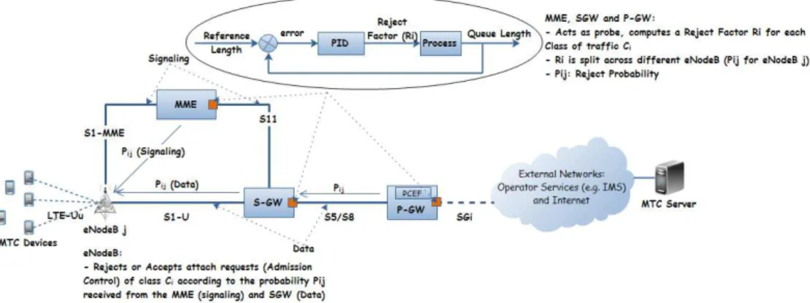
Practically, we use a queue monitoring technique based on a PID controller. The PID con-troller in a queue detects congestion and defines the Admission Control parameters. These pa-rameters have to be applied (in the input of the system) to get the desired value of the queue length. In fact, the PID controller will take as an input the current queue length and a reference value. It produces the control variable which is a Reject Factor. The Reject Factor represents the sum of the amount of traffic to be rejected in comparison to the actual traffic to reach the reference value of the queue (the incoming traffic is the input of the system). The traffic to reject is the traffic that causes the system (the queue) to deviate from the reference value. This controller is implemented in every CN node (MME, S-GW and P-GW).

In congestion controller we used to see in literature, the focus is made on TCP mainly. This means that the traffic reducing is done by mean of the TCP congestion windows or any TCP-friendy mechanism for UDP. In the context of our work (LTE networks), the congestion reducing is done by mean of rejecting connexions in the radio part when congestion is experienced at any level of the network. This means that congestion is quantified in a probe system (the Core Network nodes). Then, decisions (congestion or not, the level of congestion) is sent back to inform about the state. The scheduling nodes (eNodeB) and the UE use the received information to reduce the number of connexions, the amount of traffic (eNodeB) and the signaling by rejecting traffic before reaching congested nodes. Moreover, UE are sent to idle states.

In literature, congestion controllers for networks in general have been proposed. For instance, Random Early Detection (RED) has been proposed by Sally Floyd et al. [38] and its variants Gentle RED [39] and Adaptive RED [40], and BLUE [41]. These congestion controllers focus on reducing the load while tolerating underutilization of resource (queue going down after congestion is experienced). The controller we propose is based on control theory. It insures a targeted utilization of the resources in the network while preventing losses. Some results and comparisons between the of PID congestion controllers and the previously cited ones are given in [20].

3.2 Congestion metrics

The congestion detection will be done in the different CN nodes (MME, S-GW and P-GW). In all the nodes, the congestion could be observed in the output links or while processing. The most noticeable is the fact that it is mostly observed in the output links. This means that the processing is generally done much faster than the capacity of forwarding to the next node. For instance, user data is forwarded from the S1 bearer to the S5 bearer (in the S-GW) after changing the encapsulation (at GTP-U level) and sent back to the IP layer.

Consequently, a congestion is materialized by a queue which is full or whose length is greater that a certain threshold. Furthermore, it is a measure of the resource utilization. In fact, a queue

(19)

which is always full and that loses packets (overflow) means that the resource (a link for instance) is over utilized, while, a queue always empty means that the resource is underutilized (if there are entities requesting the resource).

Let’s note that the congestion controller we propose, as we will see it in more details in the paragraphs to come, could be used at different levels of the protocol stack where data is enqueued for processing or after being processed. In fact, the considered metric is queue length whatever the enqueued elements are.

One question could be why queue length and not the delay. In fact, the queue length is the most utilized in literature. For instance RED [38] and its variants Gentle RED [39] and Adaptive RED [40] and many others (BLUE [41]...) use the queue length as congestion metric. However, they use the average values of queue length (see [38] for examples). In our case, when combined with the PID controller, we use the evolution of the queue through the time.

In our case, we are interested in congestion in the Uplink direction. This means the traffic from the MTC Devices to the Core Network. In fact, most of the data is sent from the MTC Devices to the servers periodically, at the occurrence of an event or after a user query. Furthermore, The signaling is generated in the Uplink direction for attach requests. This doesn’t mean that we ignore the downlink. The point is that congestion is mostly observed in the uplink direction in the context of MTC in contrary to non-MTC traffic (for instance, video streaming).

Furthermore, in the context of MTC applications, MTC Devices generally go to idle sates (EMM IDLE) (EMM holds for EPC Mobility Management). In fact, it is done in respect to the property of low energy consumption. When they need to send or receive data and/or signaling, they attach to the network. Therefore, the signaling congestion is quantified in the eNodeB and MME by the lengths of the queues of the corresponding packets. During the rest of the time, they go to idle state.

The signaling congestion is the most to be observed than the data congestion. In fact, since each data sent follows a signaling attach procedure, we are to observe a lot of signaling from MTC Devices than the Data. This is the opposite of the non MTC Devices where the amount of data is very important (voice call, video conference) in comparison to the amount of signaling.

3.3 Congestion-Aware Admission Control (CAAC)

As we presented earlier, and applied in the context of MTC applications, we define 3 kinds of applications classified in the rising order of priority: Time Driven, Query Driven and Event Driven. We handle congestion at the IP level. The first thing to do is to define a schema for packet marking. This means that according to the type of the application, the packets are marked by setting for instance the ToS (Type of Service). Then, according to the priority, the packets are scheduled in the core network part (MME, S-GW and P-GW). Our congestion controller

will prevent congestion by computing a Reject Fractor Rrej. Rrej depends on the packet class.

The advantage with this approach is the fact that congestion is well defined (queue length) and accessible for measurement. The congestion notifications are sent back to the downstream nodes. This is for instance from the S-GW to the eNodeB. Practically we send a Reject Probability according to the congestion experienced in the node. The whole approach is illustrated in Figure 9.

(20)

Figure 9: General Overview of the Solution

connected to the same MME, S-GW and P-GW. Both of the MME, S-GW and P-GW receive the traffic coming from the n eNodeB. It is worth to recall that all traffic is IP, both data and signaling. All what differentiates it is the marking we use (the ToS (Type of Service), port number,...). We summarize in the following what happens in each node. Lets take the example of the MME in case of signaling.

In the MME, a PID controller is implemented for each queue of class of traffic Ci. This means

that for each class, the corresponding packets are enqueued in a separate queue. A queue moni-toring technique using a PID controller is implemented for each class of traffic (the corresponding

queue). It computes the Reject Factor we call Ri as follows :

Ri(k) = Ri(k − 1) + Kp(e(k) − e(k − 1) + KiTse(k) +

Kd

Ts

(e(k) − 2e(k − 1) + e(k − 2)) (3)

where : Q(k) : the queue length at the kth _{sampling instant (t = k ∗ T}

s)

Qref : the reference queue length we are targeting

e(k) = Q(k) − Qref

Ts: Resampling period

Kp : Proportional Gain, Ki : Integrative Gain, Kd: Derivative Gain

Ri(k) ∈ ] − ∞, +∞[

However, a negative value of the Reject Factor have no significance in our case. Therefore, it is set to 0 if bellow as follows:

Ri(k) = max (Ri(k − 1) + Kp(e(k) − e(k − 1) + KiTse(k) +

Kd

Ts

(e(k) − 2e(k − 1) + e(k − 2)) , 0) (4) Then, according to the sources or what we called the downstream nodes (eNodeB in this case),

a dedicated Reject Probability Pi,j (for eNodeB j) is computed as follows:

where n is the number the downstream nodes

(21)

As Pi,j is a probability, it is set to 1 if above. This gives : Pi,j = min( traf f ici,j Pn k=0traf f ici,k .Ri,1)

Finally, Pi,j depends on time since Ri does. it is given by:

Pi,j(l) = min(

traf f ici,j

Pn

k=0traf f ici,k

.Ri(l), 1)

By doing so, we ensure a fairness between nodes and non-starvation of certain nodes.

The computed probabilities Pi,j are then sent back to the downstream nodes (eNodeB). The

eNodeBs implement the Admission Control mechanism. They reject traffic after having the true

information of the traffic in the Core Network part summarized in Pi,j. Hence, only (1−Pi,j)∗100%

of the incoming traffic (from UE) is accepted. The Admission Control is implemented in each eNodeB j as follows :

On receipt of a packet (attach request) of class i from a UE

if (unif (0, 1) < Pi,j)

then

Reject the request (attach request) else

Forward the request to the MME endif

The interpretation of the Reject Factor is the amount of packets (from the class) to be rejected to reach the reference value of the queue length. For instance, it represents the sum of the reject

probabilities in the downstream nodes in the case where ∀j in {1 .. n} Pi,j ∈ ]0, 1[. In fact

Pn j=0Pi,j =Pnj=0 traf f icj Pn k=0traf f ick.Ri = Pn j=0traf f icj Pn k=0traf f ick.Ri = Ri

However, this is not correct in that case where Pi,j = 0 or Pi,j = 1 (because of the rounding

we perform to get the probabilities Pi,j)

4 Performance evaluation

4.1 Simulation model

We use ns-3 [3] to implement our solution and to carry out the simulations. The results are plotted using gnuplot. The choice of ns-3 was made after we used Opnet [42] for one month.

(22)

Opnet seamed to be not well adapted. In fact, it is designed to simulate as much as possible all the protocols of LTE. However, through our work, simulations take a long time before failing. It doesn’t succeed to handle all the load we impose.

Therefore, we focused on ns-3, a well done simulator. In fact, ns-3 is designed to be a simulator for research instead of business matters. It is open source, done by research for research. However, it is a new simulator and doesn’t have any dependency with its predecessor ns-2. It is developed in C++ and offers all the opportunities of Object Oriented Programming paradigm.

Under ns-3, we implemented the signaling and data messages as being application level mes-sages. The congestion is quantified using the Queue at the output of the IP layer. It represents outgoing queue from the IP layer and the network device queue (Link Layer). This is an abstrac-tion of the congesabstrac-tion we can have at any level of the architecture. For instance, we can replace it by a NAS (Non Access Stratum) level queue to handle the congestion at the NAS level (We consider the incoming queue of the NAS Server in the MME).

We developed a PIDQueue as being a module that has a Drop Tail Queue augmented by a PID controller. It is an extension (inherits) of the Queue class in ns3.

4.2 Test scenarios

We test in the following scenarios the case of Event Driven and Time Driven Applications. The sequence diagram of the generated traffic is illustrated in Figure 3.

In an Event Driven Application, the nodes likely to send the traffic at the same time are the nodes located in the same cell or in neighboring cells. In fact, when a fire is detected for instance in a region, the nodes that detect it are likely to be in the same area. This means that they are covered by the same eNodeB. Here we can, also, consider the case of VPN where and eNodeB plays the role of several logical eNodeB, so the nodes that communicate to signal the events could be from different cells.

Note that only one data packet is sent each time an attach procedure succeeds. It is a choice to simplify the simulations since we are more interested in signaling.

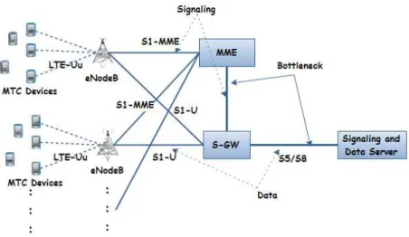
First, lets present the generic topology we use for simulations. It is illustrated in Figure 10. At this level of our work, we are not interested in the radio part of the network. Thus, we assume that the eNodeB can handle the amount of traffic the UE generate. The core of our work deals with the congestion in the Core Network part as we explained before. The eNodeB are used to implement the Admission Control.

Consequently, the links between eNodeB and the MME and the S-GW are over-sized. We consider 10 Gbps point to point links. However, the links that are likely to represent bottlenecks are set to low rates, for instance, 1500 Kbps for the link between the MME and the SGW (signaling congestion) and 3000 Kbps between the S-GW and the data and signaling server. The rest of the parameters of simulations, we consider data and signaling packets of the same size (700 bytes).

We tested our approach in four scenarios: in case of uniform traffic, in case of bursts, in case of uniform traffic with bursts and a random traffic. In fact, bursts are what characterize MTC applications since devices are likely to send data at synchronized periods (timer fired or event occurred).

(23)

Figure 10: LTE Network Testing Topology

Not that in all the scenarios to come, we consider the UE as begin MTC Devices that generate traffic corresponding to applications of the same class. Furthermore, only traffic of this class is simulated. This is realistic since we can consider the case where VPN are used. For instance, we consider that each class of traffic is sent on a separate VPN.

4.2.1 Bursty traffic

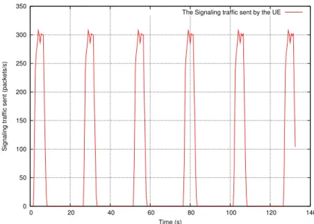
Test configuration In this first scenario, we consider bursty traffic. The pattern of the traffic

generated by the MTC Devices is illustrated in Figure 11.

The other parameters of the simulation are summarized in Table 2

Parameter Value Details

nMME 1 the number of MME

nSGW 1 the number of MTC Devices per cell

neNB 10 the number of eNodeB connected to each MME

nUEperCell 150 number of MTC Devices per cell

Kp 0.032 the PID Queue (MME) Proportional Gain

Ki 0.00051 the PID Queue (MME) Integrative Gain

Kd 0.000312 the PID Queue (MME) Derivative Gain

Ts 0.01 s the PID Queue (MME) Resampling period

Buf f er size 100 the buffer size (maximum queue length) (packets)

Ref erence 50 the PID Queue (MME) Reference length (packets)

Table 2: Simulation parameters in case of Bursty traffic

Results The evolution of the Reject Factor (Ri) in the MME and the Reject Probability (Pi,j)

in each eNodeB is illustrated in Figure 12. We note that the Reject Factor responds to the traffic received. Furthermore, the eNodeB forward approximately the same amount of traffic. Hence,

(24)

0 50 100 150 200 250 300 350 0 20 40 60 80 100 120 140

Signaling traffic sent (packets/s)

Time (s)

The Signaling traffic sent by the UE

Figure 11: The Signaling traffic generated by the MTC Devices in case of bursty traffic

the Reject Probabilities are similar and represent around 1

10Ri. This is what we expect since the

eNodeB forward the same amount of traffic.

The evolution of the Reject Factor depending on signaling traffic received and queue length in the MME is given in Figure 13. What we note is the fact that the Reject Factor adapts to the amount of traffic received (that impacts naturally the queue length). We note also that the queue length is maintained around the reference by the PID controller and the eNodeB that rejects traffic. Furthermore, the bursts are well handled since neither overflow nor underutilization are observed.

In fact, our approach handles well the congestion. The comparison with a case where we use drop tail queue are illustrated in Figure 14. We note that when using the PID queue in the MME and the Admission Control at the eNodeBs level, the queue length is maintained around the reference (50 packets) and no packets are dropped (lost), whereas, with a drop tail queue, bursts affect the queue length (over-utilization) and packets are dropped (lost) (Figure 14, (a) and (b)). At some points, 49 packets/s are lost. Furthermore, the amount of signaling forwarded by the eNodeBs is reduced since the same amount of data is sent for both of them (Figure 14, (c) and (d)). This means that we succeed to reduce the amount of signaling while keeping the same goodput (data sent thanks to the signaling).

4.2.2 Uniform traffic

Test configuration In the second scenario, the attach requests are uniformly distributed over

the time. This means that all the connexions are independent from each other. The signaling traffic generated by the UE is illustrated in Figure 15. This holds for applications independent from each other that generates traffic toward the MTC servers in such a way that no bursts are observed. This could be a real scenario if some synchronization is done at the application level. For instance, in a time driven application, nodes are scheduled in different intervals to prevent

(25)

0 0.5 1 1.5 2 2.5 0 20 40 60 80 100 120 140 160 180 Reject Factor Time (s)

Reject Factor Evolution in the PID Queue in the MME

(a) Reject Factor in the MME

0 0.05 0.1 0.15 0.2 0.25 0 20 40 60 80 100 120 140 160 Reject Probability Time (s)

Reject Probability Evolution in eNB 0 Reject Probability Evolution in eNB 1 Reject Probability Evolution in eNB 2 Reject Probability Evolution in eNB 3 Reject Probability Evolution in eNB 4 Reject Probability Evolution in eNB 5 Reject Probability Evolution in eNB 6 Reject Probability Evolution in eNB 7 Reject Probability Evolution in eNB 8 Reject Probability Evolution in eNB 9

(b) Reject Probability in the eNodeB

Figure 12: The Reject Factor evolution in the MME and the Reject Probabilities in the different eNodeBs in case of Bursty traffic

0 50 100 150 200 250 300 350 0 20 40 60 80 100 120 140 160 180 0 0.5 1 1.5 2 2.5

Signaling traffic received (packets/s), Queue Length (Packets)

Reject Factor

Time (s)

The signaling traffic sent by the UE (packets/s) The signaling traffic received at the MME (packets/s) The PID Queue Length in the MME (Packets) Reject Factor Evolution in the PID Queue at the MME

Figure 13: The Reject Factor evolution depending on the signaling traffic received and the queue length in the MME in case of Bursty traffic

(26)

0 20 40 60 80 100 0 20 40 60 80 100 120 140

Queue Length (Packets)

Time (s)

PID Queue, reference legth = 50 Drop Tail Queue

(a) Queue Length in the MME

0 5 10 15 20 25 30 35 40 45 50 0 20 40 60 80 100 120 140 160

Dropped Packets (Packets/s)

Time (s)

PID Queue, reference length = 50 Drop Tail Queue

(b) Dropped packets in the MME

0 50 100 150 200 250 300 350 0 20 40 60 80 100 120 140

Signaling traffic received (packets/s)

Time (s)

(c) Signaling traffic received in the MME

0 50 100 150 200 250 300 0 20 40 60 80 100 120 140

Data traffic received (packets/s)

Time (s)

(d) Data traffic received in the S-GW

Figure 14: Comparison between the case where a PID queue and drop tail queue are used in the MME in the case of Bursty traffic

(27)

0 50 100 150 200 250 300 350 0 20 40 60 80 100 120 140 160

Time (s)

Figure 15: The Signaling traffic generated by the MTC Devices in case of Uniform traffic bursts.

The other parameters of the simulation are summarized in Table 3.

Table 3: Simulation parameters in case of Uniform traffic

Results The evolution of the Reject Factor (Ri) in the MME and the Reject Probability (Pi,j)

in each eNodeB is illustrated in Figure 16. We note again that the Reject Probabilities are quite similar. Furthermore, they respond to the amount of traffic generated by the UE.

The evolution of the Reject Factor depending on signaling traffic received and queue length in the MME is given in figure 17. Again, we note that the Reject Factor adapts to the amount of traffic received (that impacts naturally the queue length). We note also that the queue length is maintained around the reference by the PID controller and the eNodeB that rejects traffic. Moreover, neither under-utilizations nor overflows are observed.

(28)

0 0.5 1 1.5 2 2.5 3 0 20 40 60 80 100 120 140 160 180 Reject Factor Time (s)

0 0.05 0.1 0.15 0.2 0.25 0.3 0 20 40 60 80 100 120 140 160 Reject Probability Time (s)

Figure 16: The Reject Factor evolution in the MME and the Reject Probabilities in the different eNodeBs in case of Bursty traffic

0 50 100 150 200 250 300 350 0 20 40 60 80 100 120 140 160 180 0 0.5 1 1.5 2 2.5 3

Reject Factor

Time (s)

Figure 17: The Reject Factor evolution depending on the signaling traffic received and the queue length in the MME in case of Uniform traffic

(29)

0 20 40 60 80 100 0 20 40 60 80 100 120 140 160

Time (s)

PID Queue, reference legth = 50 Drop Tail Queue

0 10 20 30 40 50 60 0 20 40 60 80 100 120 140 160

Time (s)

PID Queue, reference value = 50 Drop Tail Queue

0 50 100 150 200 250 300 350 0 20 40 60 80 100 120 140 160

Time (s)

0 50 100 150 200 250 300 0 20 40 60 80 100 120 140 160

Time (s)

Figure 18: Comparison between the case where a PID queue and drop tail queue are used in the MME in case of Uniform traffic

The comparison with a case where we use a drop tail queue are illustrated in Figure 18. We note that when using the PID queue in the MME and the admission control at the eNodeBs, the queue length is maintained around the reference (50 packets) and no packets are dropped (lost), whereas, with a drop tail queue, many packets are lost (45 packets/s in average) (Figure 18, (a) and (b)). Furthermore, the amount of signaling forwarded by the eNodeBs is reduced since the same amount of data is sent for both of them (Figure 18, (c) and (d)). This means that we succeed to reduce the amount of signaling while keeping the same goodput (data sent thanks to the signaling).

4.2.3 Uniform traffic with bursts

Test Configuration The third scenario is a combination of the two previous ones. The MTC

Devices send traffic uniformly over the time. This is likely to be a Time Driven application. Sometimes, bursts are observed (an event occurring the monitored area). The signaling traffic generated by the MTC Devices is illustrated in Figure 19.

(30)

0 50 100 150 200 250 300 350 0 20 40 60 80 100 120 140 160

Time (s)

Figure 19: The Signaling traffic generated by the MTC Devices in case of Uniform traffic with bursts

The other parameters of the simulation are summarized in Table 4.

Table 4: Simulation parameters in case of Uniform traffic with bursts

Results The evolution of the Reject Factor in the MME and the Reject Probability in each

eNodeB is illustrated in Figure 20.

The evolution of the Reject Factor depending on signaling traffic received and queue length in the MME is given in figure 21. What we note is the fact that the Reject Factor adapts to the amount of traffic received (that impacts naturally the queue length). We note also that the queue length is maintained around the reference by the PID controller and the eNodeB that rejects traffic. Moreover, the bursts introduced are handled by the controller.

Furthermore, our approach handles well the congestion. The comparison with a case where we use drop tail queue are illustrated in Figure 22. We note that when using the PID queue in

(31)

0 0.5 1 1.5 2 2.5 3 0 20 40 60 80 100 120 140 160 180 Reject Factor Time (s)

0 0.05 0.1 0.15 0.2 0.25 0.3 0 20 40 60 80 100 120 140 160 Reject Probability Time (s)

Figure 20: The Reject Factor evolution in the MME and the Reject Probabilities in the different eNodeBs in case of Uniform traffic with bursts

0 50 100 150 200 250 300 350 0 20 40 60 80 100 120 140 160 180 0 0.5 1 1.5 2 2.5 3

Reject Factor

Time (s)

Figure 21: The Reject Factor evolution depending on the signaling traffic received and the queue length in the MME in case of Uniform traffic with bursts

(32)

0 20 40 60 80 100 0 20 40 60 80 100 120 140 160

Time (s)

0 10 20 30 40 50 60 70 0 20 40 60 80 100 120 140 160

Time (s)

0 50 100 150 200 250 300 350 0 20 40 60 80 100 120 140 160

Time (s)

0 50 100 150 200 250 300 0 20 40 60 80 100 120 140 160

Time (s)

Figure 22: Comparison between the case where a PID queue and drop tail queue are used in the MME in case of Uniform traffic with bursts

the MME and the admission control at the eNodeBs, the queue length is maintained around the reference (50 packets) and no packets are dropped (lost), whereas, with a drop tail queue, bursts affect the queue length and packets are dropped (at some points, 70 packets/s are lost) (Figure 22, (a) and (b)). Furthermore, the amount of signaling forwarded by the eNodeBs is reduced since the same amount of data is sent for both of them (Figure 22, (c) and (d)). This means, again, that we succeed to reduce the amount of signaling while keeping the same goodput (data sent thanks to the signaling).

4.2.4 Random traffic

Test Configuration In the fourth scenario, the MTC Devices send traffic randomly over the

time. The signaling traffic generated by the MTC Devices is illustrated in Figure 23. We retrieve again the bursts and other patterns. This also a traffic likely to be observed if we deploy many applications independent from each other.

(33)

0 50 100 150 200 250 300 350 400 0 20 40 60 80 100 120 140 160 180

Time (s)

Figure 23: The Signaling traffic generated by the MTC Devices in case of Random traffic

Table 5: Simulation parameters in case of Random

Results The evolution of the Reject Factor in the MME as well as the Reject Probability in

each eNodeB is illustrated in Figure 24.

The evolution of the Reject Factor depending on signaling traffic received and queue length in the MME is given in figure 25. What we note is the fact that the Reject Factor adapts to the amount of traffic received (that impacts naturally the queue length). We note also that the queue length is maintained around the reference by the PID controller and the eNodeB that rejects traffic. The bursts noticed are handled by the controller.

Again, our approach handles well the congestion. The comparison with a case where we use drop tail queue are illustrated in Figure 26. We note that when using the PID queue in the MME and the admission control at the eNodeBs, the queue length is maintained around the reference (50 packets) and no packets are dropped (lost), whereas, with a drop tail queue, bursts affect the queue length and packets are dropped (at some points (between 48 and 53s), 90 packets/s are

(34)

0 0.5 1 1.5 2 2.5 3 3.5 0 20 40 60 80 100 120 140 160 180 Reject Factor Time (s)

0 0.05 0.1 0.15 0.2 0.25 0.3 0.35 0 20 40 60 80 100 120 140 160 Reject Probability Time (s)

Figure 24: The Reject Factor evolution in the MME and the Reject Probabilities in the different eNodeBs in case of Uniform traffic with bursts

0 50 100 150 200 250 300 350 400 0 20 40 60 80 100 120 140 160 180 0 0.5 1 1.5 2 2.5 3 3.5

Reject Factor

Time (s)

Figure 25: The Reject Factor evolution depending on the signaling traffic received and the queue length in the MME in case of Random traffic