Comparison of Field Transfer Methods between two meshes

ECCM 2010

Comparison of Field Transfer Methods between two meshes

P. Bussetta, J-P. Ponthot

LTAS MN2_{L, Aerospace & Mechanical Engineering Department,} Université de Liège, Liège (Belgium) {P.Bussetta,JP.Ponthot}@ulg.ac.be

1

Introduction

In many cases, the numerical computation of mechanical problem with Finite Element Method has to transfer some information between two different meshes [1, 2, 3, 4]. For example, if a remeshing is needed or if several meshes are used (e.g. one for a thermal problem and another one for a mechani-cal problem). In spite of the research on the Transfer Methods, none of them has been so far clearly established as the best. Each method has advantages and disadvantages. Many problems can happen during the field transfer, like the minimization of the numerical diffusion, the value of the field on the boundaries, etc.

This paper compares on the one hand the performances of the Field Transfer Method by classical interpolation with on the other hand one using Mortar Elements. The comparison of the two methods is based on two indicators: the numerical diffusion and the evaluation of the field on the boundaries. In this paper, only the continuous fields are considered.

2

Definition of the problem

In this paper a problem is computed with theFiniteElementMethod. During the computation, a remesh-ing is needed. To continue the computation, the field T evaluated on the old mesh, is needed on the new mesh. The evaluation of the field T on the old mesh is noted Told. This one is defined thanks to nodal values (T_•old). The old mesh is composed of nold_e elements and nold_n nodes. The value of Told on each element eold is written as:

Told= nelem n

∑

where Nold_j is the shape function of the node j and nelem_n the number of node of the element.

The value of this field T on the new mesh is noted Tnew. The new mesh is formed of nnew_e elements and nnew_n nodes. Like Told, Tnewis defined thanks to the nodal values (noted T_•new) and the value on each element of the new mesh enewis as:

Tnew= nelem n

∑

The aim of the transfer method is to define the nodal value of Tnew on the new mesh (T_•new). The properties of the transfer method should be:

• weak numerical diffusion, • conservation of the extrema, • easily treatment of the boundaries.

3

Transfer Methods

The Field Transfer Method makes the link between the two discretisations. The reliability of the field on the new mesh is directly linked with the transfer method used.

3.1 Interpolation Method

The interpolation method is the most commonly used. The value of Tnewat each node of the new mesh (T_•new) is equal to the interpolation of the nodal values of the old mesh (Told; [2, 3]). The computation is done in two steps:

• Firstly, for each node of the new mesh a search is done to find the element of the old mesh eold in which the node lies inside.

• Then, the value of the field on this node is computed by interpolation of the nodal values of the element eold, as:

T_•new= Told₌ nelem n

∑

This method does not deal with the elements of the new mesh. These elements have no influence on the value of the field. The transfer is done from a mesh to a node for all nodes of the new mesh. This method conserves the extrema, but due to geometrical approximations, some nodes on the boundary can be outside of the old mesh. So, a special treatment is requered for the boundaries.

3.2 Weak Form Method

The second method (using Mortar Element [1]), is based on a weak conservation form of the field. The new nodal values are not directly computed. The field on the new mesh is evaluated considering that the integral of the difference between the value of the fields on the new mesh and the value on the old mesh is null ([1, 5, 6, 7]). The computation of this integral is done over the new mesh, as:

nnewe

∑

where enew_{is a element of the new mesh, and f is a weighting function defined on each element e}new_{as :}

f = nelem n

∑

The nodal value of the function f (noted f_•) can take any value. The equation (4) can be written like: nnew n

∑

∑

∑

Where N_AB1 and N_AC2 are the mortar elements defined as:

N_AB1 = nnew e

∑

∑

where N_inewis the shape function of node i (A or B) in the element enew, and N_Cold is the shape function of the node C in the element of the old mesh intersected by the element enew.

3.2.1 Computation of mortar element

The first Mortar Element (N_AB1 ) is the integral over the elements of the new mesh of the product of two shape functions of one of these elements. So, this value is computed by numerical integration over each element of the new mesh enewas:

N_AB1 (enew) =

∑

ip

N_Anew(ip)N_Bnew(ip) (8)

The value of the Mortar Element N_AB1 is the sum of the contribution of each element of the new mesh:

N_AB1 =

nnewe

∑

enew₌₁

N_AB1 (enew) (9)

The evaluation of the second Mortar Element (N_AC2 ) is more complex because of the shape function of the node C on the element of the old mesh (N_Cold). The sum of the shape functions N_Coldon each element of the old mesh is not a polynomial function on each element of the new mesh (enew). A numerical and an exact integration are used to compute this Mortar Element.

Numerical integration The mortar element is computed by numerical integration over each element of the new mesh. For the element of the new mesh enew, the computation is done with nip integration points and the part of the mortar element is defined by:

N_AC2 (enew_{) =} n

ip

∑

ip=1

N_Anew(ip)Nold

C (ip) (10)

Where N_Coldis the shape function of the node C on the element of the old mesh including the integration point ip. The numerical integration suppose that the sum of the shape function of the node C can be evaluated by a polynomial function on each element of the new mesh.

Exact integration Each element enewof the new mesh is divided in nsub_e elements, as each part (esub) is only over one element of the old mesh. So, on each element esub, N_Coldis a polynomial function.

N_AC2 (enew) = nsub e

∑

Finally, the mortar element can be computed exactly by numerical integration over each part of the element enew, because is an integration of polynomial function.

N_AC2 (enew_{) =}

nsub e

∑

esub₌₁

∑

N_Anew(ip)Nold C (ip)

!

(12)

The exact integration of mortar element considers all intersections between the element of the new mesh and the elements of the old mesh. However, with the numerical integration, the mortar elements are evaluated in function of the intersection in which the integration point lies inside. So, the intersections than are smaller than the influence area of the integration point can be ignored. Like the Mortar Element

N_AB1 , the value of the Mortar Element N_AC2 is the sum of the contribution of each element of the new mesh:

N_AC2 = nnew e

∑

3.2.2 Evaluation of the field on the new mesh

Global solving The equation (6) can be written as:         f1 .. . fA .. . fnnew n         T        N₁₁1 · · · N1B1 · · · N1n1new n .. . ... ... N_A11 · · · NAB1 · · · NAn1 new n .. . ... ... N_n1new n 1 · · · N 1 nnew n B · · · N 1 nnew n nnewn                 T₁new .. . T_Bnew .. . T_nnewnew n         =         f1 .. . fA .. . fnnew n         T         ∑nold C=1N1C2 TCold .. . ∑nold C=1NAC2 TCold .. . ∑noldn C=1Nn2new n CT old C          (14)

This relation is verified for any nodal value fAof the function f , so the equation to solve can be written:

        N₁₁1 · · · N1B1 · · · N1n1new n .. . ... ... N1 A1 · · · NAB1 · · · NAn1 new n .. . ... ... N_n1new n 1 · · · N 1 nnew n B · · · N 1 nnew n nnewn                 T₁new .. . T_Bnew .. . T_nnewnew n         =          ∑nold C=1N1C2 TCold .. . ∑nold C=1NAC2 TCold .. . ∑nold n C=1Nn2new n CT old C          (15)

The size of this equation is equal to the number of node of the new mesh. In addition the solution of this equation cannot certify the conservation of extrema.

Local solving To obtain a local system, a diagonal matrix is used. The value of the diagonal term is equal to the sum of the line (or the column, because the matrix is symmetric). This is totally equivalent to the row-sum technique used to lump mass matrix in explicit time integration method. So the value of the field T on each node is done by:

T_Anew= noldn

∑

∑

With this method, the weak conservation of the field is done in a cell composed of the elements of the new mesh including the node A. This technique increases the area of computation of nodal value and in the same time the numerical diffusion. But, in opposition of the global solving, the local solving conserves the extrema.

To sum up, the evaluation of the field T is directly done at the node of the new mesh (T_•new) on a function of the elements of the new mesh (N_AB1 ), the nodal values and the elements of the old mesh (T_•old and N_AC2 ).

4

Examples

The comparison of the two methods is done on two dimensional academic examples. Two examples are treated. These exemples expose the numerical diffusion and the evaluation of the field on the boundaries of the transfer methods. The meshes are composed of quadrilateral elements. With the Weak Form Method, the evaluation of the Mortar Element N_AB1 is done by numerical integration using two Gauss points in each direction. For the numerical integration, the Mortar Element N_AC2 is evaluated with five Gauss points in each direction on each element of the new mesh. For the exact integration, the evaluation of the Mortar Element N_AC2 is done using six Gauss points on each triangle of the subdivision of the element (to exact integration of quadratic function).

4.1 Numerical diffusion

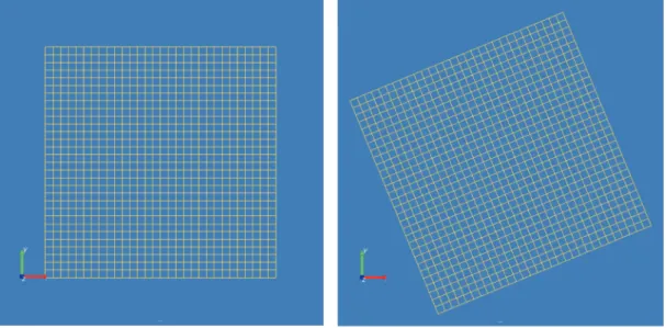
The numerical diffusion of the transfer operator is studied by the transfer of a field between two identical squares. The new mesh is equal to the old after a rotation ofπ/8. The square’s sides are meshed by 30 elements (see figure 1). The exact value of the field is of a hundred inside a circle and null outside. The centre of the circle is identical to the centre of the square and the radius is the half of the side’s square. This field is defined thanks to the nodal values. This value is equal to the exact value of the field. The figure 2(a) show the evaluation of this field on the initial mesh.

(a) Old mesh (before the first transfer) (b) New mesh (after the first transfer)

(a) Initial value (b) Interpolation Method

(c) Local Weak Form Method (numerical integration) (d) Local Weak Form Method (exact integration)

(e) Global Weak Form Method (numerical integration) (f) Global Weak Form Method (exact integration)

Figure 2: Numerical diffusion after twenty transfers: by Interpolation and Weak Form Method (numeri-cal and exact integration of the Mortar Elements)

The evaluation of the field has been transferred twenty times during the rotation and after that, the comparison of the numerical diffusion is done (see figures 2(b), 2(c), 2(d), 2(e), 2(f), and 3). These figures show that the method that minimizes the numerical diffusion is the Global Weak Form Method, but this one does not conserve the extrema. The weak conservation of the field introduces oscillations around a steep variation (see figure 2(e), 2(f), and 3). The numerical diffusion is the most important with the Local Weak Form Method because the area of influence of a given node is larger. The computation of the nodal value of the new mesh is done in a cell composed by all the elements including this node (see equation 16). The weak conservation of the field is done on this cell.

In this case, the difference between the numerical and the exact integration of the Mortar Elements is not significant (see figures 2(c), 2(d), 2(e), 2(f), and 4(a)). With the Global Weak Form Method, the numerical integration of the Mortar Element absorbs the numerical wave (see figures 2(e), 2(f), and 4(b)).

5 10 15 20 25 30 0 20 40 60 80 100

Value of Nodal Field

Initial value Interpolation Local Weak Global Weak

(a) After one transfer

5 10 15 20 25 30 0 20 40 60 80 100

Value of Nodal Field

Initial value Interpolation Local Weak Global Weak

(b) After twenty transfers

Figure 3: Numerical diffusion: by Interpolation and Weak Form Method (numerical integration of the Mortar Elements) 5 10 15 20 25 30 0 20 40 60 80 100

Value of Nodal Field Initial value numerical int. exact int.

(a) Local Weak Method

5 10 15 20 25 30 0 20 40 60 80 100

Value of Nodal Field Initial value numerical int. exact int.

(b) Global Weak Method

Figure 4: Numerical diffusion of Weak Form Method after twenty transfers

4.2 Influence of boundaries

To study the influence of the boundaries, a mesh of a disc with a hole is used. Like the first problem, the new mesh is equal to the old after rotation ofπ/8. The half circle is divided in fifteen elements and the

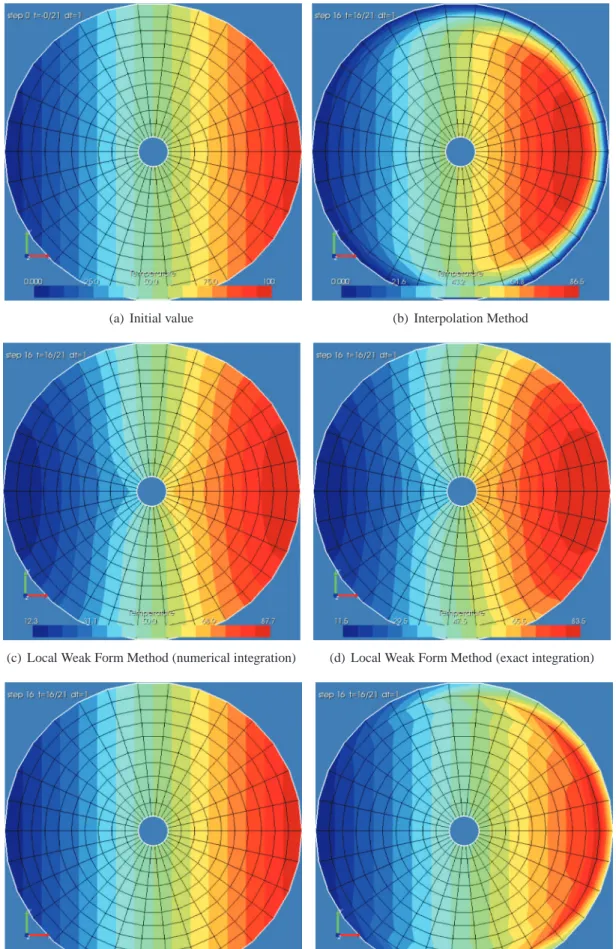
radius in ten (see figure 5). The exact value of the field is a linear function of the abscissa, the minimal value is zero and the maximal is hundred (see figure 6(a)). This field is defined thanks to the nodal values. The difficulty is that in the general case, the nodes on the boundaries of the new mesh are not always inside an element of the old mesh.

(a) Old mesh (before the first transfer) (b) New mesh (after the first transfer)

Figure 5: Meshes for the first transfer

Figures 6 show the exact value of the field (figure 6(a)) and the value of the field after sixteen transfers (one revolution, figures 6(b), 6(c), 6(d), 6(e), 6(f), and 7). This problem proves that the Interpolation Method requires a special technique to deal with the boundaries. The nodes located on the boundaries of the new mesh do not lie inside any element of the old mesh, so the value resulting the sample interpolation method is null (see figure 6(b) and 7). This problem does not appear with the Weak Form Method and the numerical integration of the Mortar Elements (see figures 6(c), 6(e), and 7), because the computation of the field is done on the integration points of the new mesh and these points generally lie inside of an element of the old mesh. In addition, the computation of the Mortar Elements by numerical integration does not consider the part of the elements that is outside of the other mesh. This explains that the Global Weak Form Method does not introduce any error after the transfer (see figure 6(e) and 7). The error after the transfer with the Local Weak Form Method is a numerical diffusion and not a wrong evaluation of the field on the boundaries (see figures 6(c) and 7).

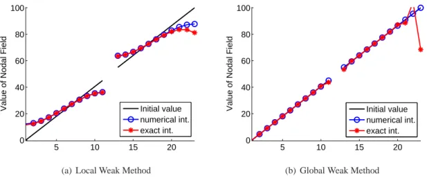
The exact integration of the Mortar Elements introduces an error of space discretisation of the bound-aries. The parts of the element of the old mesh that do not lie inside any element of the new mesh are not considered on the Mortar Elements. In the same time, the parts of the element of the new mesh that do not lie inside any element of the old mesh are considered and the value of the field inside is null. So, the integral of the field over the new mesh is not equal to the integral over the old mesh. This error impairs the quality of the solution (see figures 6(c), 6(d), 6(e), 6(f), and 8).

(a) Initial value (b) Interpolation Method

(c) Local Weak Form Method (numerical integration) (d) Local Weak Form Method (exact integration)

(e) Global Weak Form Method (numerical integration) (f) Global Weak Form Method (exact integration)

Figure 6: Numerical diffusion after sixteen transfers (one revolution): by Interpolation and Weak Form Method (numerical and exact integration of the Mortar Elements)

5 10 15 20 0 20 40 60 80 100

Value of Nodal Field

Initial value Interpolation Local Weak Global Weak

(a) After eigth transfers (half of revolution)

5 10 15 20 0 20 40 60 80 100

Value of Nodal Field

Initial value Interpolation Local Weak Global Weak

(b) After sixteen transfers (one revolution)

Figure 7: Numerical diffusion: by Interpolation and Weak Form Method (numerical integration of the Mortar Elements) 5 10 15 20 0 20 40 60 80 100

Value of Nodal Field Initial value numerical int. exact int.

(a) Local Weak Method

5 10 15 20 0 20 40 60 80 100

Value of Nodal Field Initial value numerical int. exact int.

(b) Global Weak Method

Figure 8: Numerical diffusion of Weak Form Method after sixteen transfers (one revolution)

5

Conclusion and future works

In conclusion, this paper presents a field Transfer Method between two different meshes: the Weak Form Method. This one evaluates the nodal value as a function of the field on the old mesh and the elements of the new mesh. This paper shows that the Weak Form Method with numerical integration of the Mortar Elements deals with complex boundaries without any specific procedure. In addition, the Global Weak Form Method minimizes the numerical diffusion, but the global computation can introduce oscillations around steep variations of the field. So, this method cannot conserve the extrema. On the other hand, the local computation increases the smoothing of the field. Indeed, the Local Weak Form Method introduces numerical diffusion because of the importance of the area of evaluation of nodal value. The aim of the future work is to extend the Local Weak Method on the three dimensional problems and reduce the area of evaluation of the nodal value to decrease the numerical diffusion.

Acknowledgements

The authors wish to acknowledge the Walloon Region for its financial support to the STIRHETAL project (WINNOMAT program, convention number 0716690) in the context of which this work was performed.

References

[1] D. Dureisseix and H. Bavestrello. Information transfer between incompatible finite element meshes: Applica-tion to coupled thermo-viscoelasticity. Comput. Methods Appl. Mech. Engrg., 195:6523–6541, 2006.

[2] P.H. Saksono and D. Peri´c. On finite element modelling of surface tension. Comput. Mech., 38:251–263, 2006.

[3] M. Ortiz and J.J. Quigley. Adaptive mesh refinement in strain localization problems. Computer Methods in

Applied Mechanics and Engineering, 90:781–804, 1991.

[4] G. Kermouche, N. Aleksy, J.L. Loubet, and J.M. Bergheau. Finite element modeling of the scratch response of a coated time-dependent solid. Wear, 267:1945–1953, 2009.

[5] M.M. Rashid. Material state remapping in computational solid mechanics. Int. j. Numer. Meth. Engng., 55:431–450, 2002.

[6] A. Orlando. Analysis of adaptative finite element solutions in elastoplasticity with reference to transfer

oper-ation techniques. PhD thesis, University of Wales, 2002.

[7] P.E. Farrell, M.D. Piggott, C.C. Pain, G.J. Gorman, and C.R. Wilson. Conservative interpolation between unstructured meshes via supermesh construction. Comput. Methods Appl. Mech. Engrg., 198:2632–2642, 2009.