53
BUILDING AND HVAC SYSTEM SIMULATION WITH THE HELP OF AN
ENGINEERING EQUATION SOLVER
S. Bertagnolio
1*, G. Masy
2, J. Lebrun
1and P. André
3 1Laboratoire de Thermodynamique, Université de Liège, Liège, Belgium
2HEPL Rennequin Sualem, Liège, Belgium
3Département des Sciences et Gestion de l’environnement, Université de Liège, Belgium.
(*) Corresponding author: [email protected]
ABSTRACT
A simplified Building-HVAC system model is presented here. It includes simplified models of building zone and of HVAC equipment.
The simplified building zone model is based on a R and C network, whose parameters are adjusted trough a frequency characteristic analysis. The implementation of the classical phenomena taking place in building dynamics is discussed.
The simplified building model is compared with more detailed models, using the BESTEST procedure. The application of the presented model to the audit of commercial buildings is also discussed.
INTRODUCTION
The calculation of energy consumptions, heating and cooling demands is often required for design, audit or commissioning of buildings and HVAC systems. Considering the number of parameters and influences which are involved in this type of calculation, it seems more rational to use a simulation model rather than hypothetical weather indexes as heating/cooling degree-days. For this targeted work, simulation tools are required to be easy-to-use, transparent, reliable, accurate enough and robust.
Modern computation tools allow to perform reliable detailed hourly and sub-hourly simulations of a given building and HVAC system. Currently, a large quantity of parameters is required to characterize the building and the coupled system. Moreover, models often work as black boxes.
A simplified Building-HVAC system model is presented here. It includes simplified models of building zone and of HVAC equipment. Only a limited number of easily identifiable parameters is required to tune these models. Their simplicity and the use of an engineering equation solver (Klein, 2002) to run the simulation ensure good robustness and full
transparency. In the first part of the paper, the implementation of the classical phenomena taking place in building dynamics (transient heat transfer, solar gains, internal gains, infrared losses) is discussed. The building model is also assessed using BESTEST procedure.
In the second part of the paper, the main components of the static HVAC system model are briefly presented.
Finally, a simulation tool developed as an auditing tool for commercial buildings and based on the developed models is briefly exposed. An example of simulation results is presented.
BUILDING MODEL
Laret (1981) proposed a building simplified model based on electrical analogy further developed by Ngendakumana (1988).
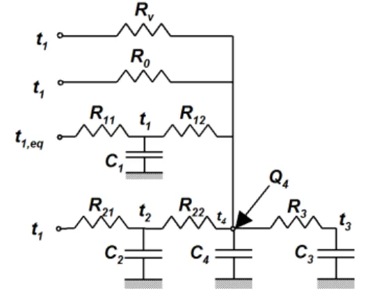
Figure 1: Building zone dynamic simplified model The model includes infiltration heat exchange Rv, transmission through low mass external walls, such as glazing, R0, and transmission through high mass external walls R21+R22 provided with a capacity C2. The indoor temperature node is connected to an indoor air capacity C4, including the air non isothermal effect.
Masy (2006) updated this model as follows (Figure 1): 1) A specific outdoor branch (R11+R12 provided with a capacity C1) is added and connected to an outdoor equivalent temperature, in order to account for solar heat gains and infrared heat losses through the roof.
2) An indoor branch was added, composed of a resistance R3 and a capacity C3, in order to account for the mass of internal walls entirely included into the zone under study. As those walls are submitted to identical temperature and heat flow signals on both surfaces, there isn’t any heat flow crossing them. They are shared in two parts, both submitted to adiabatic boundary conditions on their internal null heat flow plane.
3) The model adjustment process includes: • Wall parameters adjustment • Wall admittances combination • Building parameters adjustment 4) The parameters of each wall are tuned using
the response of the model to a sinusoidal input (Figure 2) instead of using its response to a step, as explained hereafter.
The window model is based on a simplified variation law used to compute the SHGC (Solar Heat Gain Coefficient) as function of the radiation incidence angle.
Solar radiation entering the zone are distributed over all the internal surfaces and injected on internal surface nodes of the RC network. Internal generated gains (lighting, appliances and heating/cooling power) are injected on the indoor node. Solar radiation absorbed by opaque walls are injected on the external surface nodes of the RC network.
Figure 2: Temperature and heat flow signals, on both sides of a wall including n layers
TUNING OF THE BUILDING MODEL
Temperature and heat flow signals acting on both sides of a wall are correlated by means equation 1.
=
2 2 2 2 2 2 1 1 1 1 1 1~
~
...
~
~
q
t
D
C
B
A
D
C
B
A
D
C
B
A
q
t
n n n n (1) 2 1~
,
~
t
t
in°C,q
~ q
1,
~
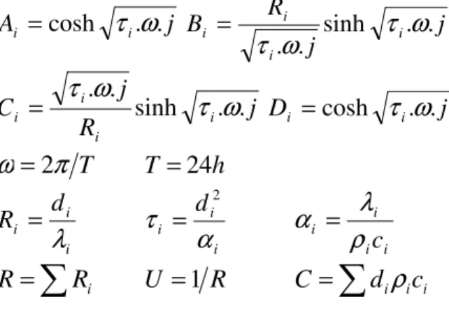
2in W/m²: temperature and heat flow sinusoidal signals expressed as complex quantities. The matrixes appearing in the product are composed of complex quantities defined as follows:j
A
i=
cosh
τ
i.
ω
.
j
j
R
B
i i i isinh
.
.
.
.
ω
τ
ω
τ
=
j
R
j
C
i i i isinh
.
.
.
.
ω
τ
ω
τ
=
D
i=
cosh
τ
i.
ω
.
j
T
π
ω
=
2
T
=
24
h
i i id
R
λ
=
i i id
α
τ
2=
i i i ic
ρ
λ
α
=
∑
=
R
iR
U
=
1
R
C
=
∑
d
iρ
ic
i id
in m,λ
i in W/m.K ,ρ
i in kg/m³,c
i in J/kg.K: thickness, thermal conductivity, density and heat capacity of each wall layer i.The matrix product of the equation (1) yields the wall reverse transfer matrix Q (2), that can be transformed in a wall admittance matrix.
= 2 2 22 21 12 11 1 1 ~ ~ ~ ~ q t Q Q Q Q q t (2) Two types of boundary conditions may then be considered in order to generate 2R1C wall models (Figure 3):
• Imposed temperature on both sides for external walls
• Imposed temperature one one side, and imposed null heat flow on the other side, for both parts of internal walls (see further)
Figure 3: 2R1C wall model including two no dimensional parameters θ and φ.
Imposed temperature conditions yield the wall isothermal admittance
A
~
ν and transmittanceK
~
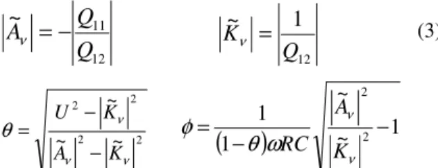
ν, whose modulus are imposed to the 2R1C model in order to adjust its θ and φ parameters (equations 3).12 11 ~ Q Q Aν =− 12 1 ~ Q Kν = (3) 2 2 2 2 ~ ~ ~ ν ν ν θ K A K U − − =
(
)
~ 1 ~ 1 1 2 2 − − = ν ν ω θ φ K A RCImposed heat flow conditions yield the wall adiabatic admittance, whose modulus and phase lag are imposed to the 2R1C model in order to adjust its θ and φ parameters (equations 4). 22 21 ~ Q Q Aν =−
( )
2 ~ . ~ ν ν θ A R A ℜ =( )
ν νω
φ
A C A ~ . . ~ 2 ℑ = (4)Before generating their 2R1C network parameters through (4), internal walls are subdivided in two parts by a null heat flow plane whose position is defined by equalizing the damping factors of two sinusoidal temperature signals acting separately on each side of the wall. The damping factor of a sinusoidal signal crossing n wall layers is defined by equation 5.
∏
= − = n i i i d d f 1 2 . expα
ω
(5) So, the resulting internal wall model is a 3R2C model. This process allowed us to define default values for θ and φ parameters as function of a wall typology. Walls are then easily described by their parameters:R=1/U, in W/m²K, C in J/m²K, θ and φ
Wall reverse transfer and admittance matrixes (2) can be deduced directly from the wall parameters:
+ + − + − = 1 . . . . ) 1 ( 1 . ) 1 ( 2 j RC j C R j C R j RC
ω
φθ
ω
φ
ω
θ
φθ
ω
θ
φ
QWall admittances are multiplied by the wall areas and the resulting matrixes are added up for each wall category in order to generate three admittance matrixes for each building zone: one for roof slabs, one for external walls, one for internal walls. The aggregated RC network model (Figure 1) is generated from the zone admittance matrixes following the same process as that used for walls (equations 3 and 4). This method
allows to generate a very simplified, light and RC network model
For the most frequent wall compositions, the adjustment parameters stay in a limited range and “standard” values are easily generated using the method previously presented. These values are then used to tune the building model. Masy has shown that the use of standard values of parameters θ and φ instead of exact values does not alter the quality of the results but simplifies greatly the parametrization work for the final user.
EXPERIMENTAL AND ANALYTICAL
VALIDATIONS
Judkoff and Neymark (1995) have proposed a complete validation methodology for building simulation models. It includes analyticial, empirical and comparative tests.
The model was tested on the experimental results provided by EMPA test cell (Figure 4) in the framework of IEA-ECBCS annex 43 research project. The cell is composed of tight insulated steel sandwich boards and the window is removed. The environment is controlled so that outdoor temperature is known. Internal heat flows are given, as well as corresponding indoor temperatures.
Figure 4: EMPA test cell (2.36 m x 2.85 m x 4.63 m) The indoor temperatures computed by the model for imposed heat flows are compared to measured indoor temperatures (Figure 5). The RMS of the error related to indoor temperature equals 0.46 K.
Figure 5: Comparison of measured (dotted black line) and computed (red line) indoor temperatures
The model is also tested by comparison with a more detailed model based on a convolution process using heat transfer functions. The comparison is performed on an office room defined in the framework of IEA-ECBCS annex 27 (Van Dijk, 2001) research project. Masy (2008) has already detailed the results of this analytical validation of the building zone model.
BESTEST COMPARISON
As mentioned above, analytical and experimental tests have been made by comparing the RC network model to the transfer function method and to experimental results.
However, comparative testing is very useful to identifiy the main differencies existing among the simplified model and some reference detailed codes. The BESTEST procedure is a comparison method used to evaluate building simulation models. This “comparative testing” approach is based on the use of benchmark test cases, generated with reference codes (BLAST, DOE-2, ESP, SRES/SUNCODE, SERIRES, S3PAS, TASE and TRNSYS). These reference models do not necessarily represent “truth” but are representative of what is commonly accepted as the current state-of-the-art in building energy simulation. (Judkoff and Neymark, 1995). Indeed, the aim of BESTEST procedure is to identify errors in the models and to guarantee consistency between them.
Two types of test-cases are proposed in BESTEST procedure :
• Diagnostic cases, attempting to isolate the effects of individual algorithm by varying parameters one by one,
• Qualification cases, representing a set of realistic lightweight and heavyweight buildings.
Only the results dealing with the qualification cases are presented hereafter.
Figure 6: BESTEST test cell
The basis of the different test cases is a rectangular room (Figure 6). The envelope characteristics,
orientation of windows and temperature setpoints vary between the different test cases.
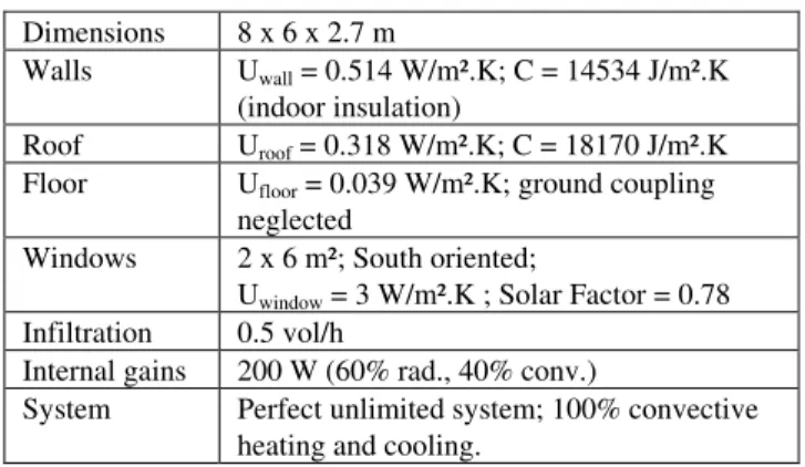
The main characteristics of the test cell are given in Table 1 for the base test-case (C600).
Table 1: Test cell description – C600 Dimensions 8 x 6 x 2.7 m
Walls Uwall = 0.514 W/m².K; C = 14534 J/m².K
(indoor insulation)
Roof Uroof = 0.318 W/m².K; C = 18170 J/m².K
Floor Ufloor = 0.039 W/m².K; ground coupling
neglected
Windows 2 x 6 m²; South oriented;
Uwindow = 3 W/m².K ; Solar Factor = 0.78
Infiltration 0.5 vol/h
Internal gains 200 W (60% rad., 40% conv.)
System Perfect unlimited system; 100% convective heating and cooling.
Basing on the C600 test-case, several variations are proposed. The main qualification cases are described in Table 2. All the proposed cases have not been considered because of the limitations of the model. Test-cases involving solar shading and equal cooling and heating setpoints have not been applied.
The meteorological data used for the simulations correspond to a cold winter (min. outdoor temperature : -24.4°C) and a dry and hot summer (max. outdoor temperature : 35°C).
Table 2: Test cell description – C600 C600 Base case
C620 C600 with one window East oriented and one window West oriented
C640 C600 with night set back to 10°C between 23:00 and 7:00
C900 - 940 C600 - 640 with heavy walls (outdoor insulation)
The integrated annual heating and cooling demands are shown, respectively, in Figure 7 and Figure 8. The building model (“EES”) provides good results for the cases 600 to 640. Some little discrepancies appear when looking at heavy-weight cases (C900 to 940). These errors could be explained by the limited order of the wall model. An accurate estimation of the interaction between indoor ambient and heavy outdoor insulated walls, would require the use of a more detailed wall model, using more than one thermal mass. However, these errors stay limited (max. 10%) and the results stay in good accordance with those provided by more detailed models.
Figure 7 : C600 to C940 – Annual Heating Demands
Figure 8 : C600 to C940 – Annual Cooling Demands The differences could also be partially explained by the use of an imperfect control for the heating/cooling system. Indeed, the heating and cooling powers must be controlled by means of proportionnal control laws to maintain the indoor set-point.
Some hourly data are also provided for comparison. These data correspond to the 4th January of the simulated year. Calculated hourly values of heating/cooling powers are shown for C600 and C900, respectively, in Figure 9 and Figure 10. Heating power is plotted in positive values while cooling power is plotted in negative values.
The simplified model provides consistent results. For the lightweight case, the calculated heating and cooling powers curves are superposed with those provided by the reference models.
As expected, for heavy inertia walls, the results are less good and, even if the global shape of the curve is respected, the superposition is not perfect. As mentioned above, this discrepancy could be explained by the low order of the wall model.
Figure 9: C600 – 4th January, H/C powers
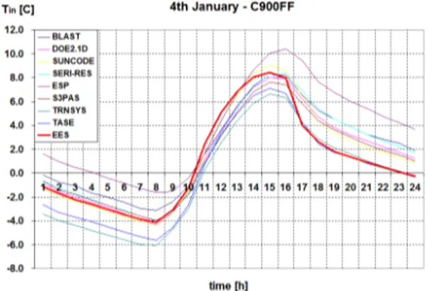
Figure 10 : C900 – 4th January, H/C powers BESTEST procedure provides also hourly values for cases C600 and C900 with floating temperature. The temperature profiles generated by the model for the testcase C900 are shown in Figure 11.
Once again, the results provided by the simplified models are in good accordance with those provided by reference models.
Figure 11: C900 – 4th January, Floating temperature The model provides results included in the range, rather close to the high limit, generated by more sophisticated models. The effects induced by inputs
and parameters variations are of the same order of magnitude as for the other building codes.
This comparative validation shows that the developed simplified building model predicts cooling and heating demands with sufficient accuracy. This simplified model is well adapted to simplified building and system simulation tools.
IMPLEMENTATION AND APPLICATION
Two simulation tools are being developed on the basis of the previous model. Both tools are developed with the help of an Engineering Equation Solver (Klein, 2002). The first one is a residential-building simulation tool (Masy, 2006), used to perform comfort analysis and energy consumptions prediction for different heating (or cooling) systems and for various control strategies. The second one is an auditing-benchmarking tool for commercial buildings.
Mono-zone Building Model
In this benchmarking tool, the previously described building model (Figure 1) is used to simulate the thermal behaviour of the whole building, surrounded by its envelope (opaque frontages, windows and roof) and including the floor slabs.
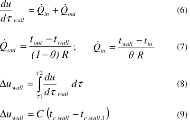
The energy storage in heavy walls is computed by the means of first order differential equation systems. The use of an equation solver allows to solve directly the equations 6 to 9. out in wall
Q
Q
d
du
&
& +
=
τ
(6)R
θ)
(1
t
t
Q
out wall out−
−
=
&
; R θ t t Q wall in in − = & (7)∫
=
∆
2 1 τ ττ
τ
d
d
du
u
wall wall (8)(
c,wall c,wall,1)
wallC
t
t
u
=
−
∆
(9)Some similar equations are used to compute the energy storage in adiabatic heavy walls. A sensible heat balance is computed on the indoor node to compute the indoor temperature. Two mass balances are used to compute CO2 and water content in the zone. More details about the implementation of the model in the equation solver will be described in further papers. The building model is then directly coupled to the HVAC system model described here after.
HVAC System Model
The system model includes most of the classical HVAC components currently available. Originally, at least two types of component models are developed (André et al., 2006) :
• complete, validated, detailed and accurate reference models (called “mother models”), used to compute components characteristics on the basis of manufacturer data,
• simplified and robust simplified models (called “daughter models”), adjusted with previously defined characteristics to run simulations, Like for the building zone, the HVAC “mother” models are validated in different ways (analytical, empirical and comparative validations). Lemort et al. (2008) presented an example of derivation of a simplified cooling coil model from a reference cooling coil model.
Using these simplified models, all the equipments (AHUs, TUs, pumps, fans, networks,…) are gathered and modelled as “global” components of each type. The connected global HVAC system model (Figure 12) includes one global Air Handling Unit model, one global Terminal Unit model and one Heating/Cooling Plant model.
Air and water networks are also modelled to take pressure drops and heat exchanges into account.
Figure 12: Building-HVAC System model scheme
The AHU model includes recovery system, economizer, filter, preheating coil, adiabatic humidifier, cooling coil, post heating coil, steam humidifier, main fan and return fan (Figure 12). Emission systems include radiators, induction or fan coil units, heating floor and cooling ceiling and are directly controlled to maintain indoor temperature. Correlation-based models, derived from “mother” reference models, are used to simulate the heat and cool production systems (conventional or condensing boilers and water or air cooled chillers). Of course, these components are never to be selected all together at the same time by the user. More details about the components models are given by André et al. (2006) and will be given in further papers.
Building and System entities are generally modeled separately, and called in a sequential way during a simulation process. This is not the case here, building and HVAC system models are directly coupled. Each HVAC system component is controlled using ideal and simple proportionnal control laws, as shown in Figure 13. This approach allows to take into account of HVAC components limited capacities and to model the interactions between the building and the system. Hourly values of indoor temperature, humidity, heating, cooling and electricity demands are computed by the model. The tool provides also performance indicators related to air quality (CO2 concentration)
and thermal comfort (Predicted Percentages of Dissatisfied) as well as gas, fuel and electricity consumptions, primary energy consumption, CO2
emissions and global energy cost, with accounting for high and low electricity rate hours.
Commercial Building Auditing Tool
When starting an audit procedure, the auditor has to collect some information about the building and the related HVAC system to be audited (building fabric, type of HVAC system, monthly energy consumptions,…). Using only this global data, the auditor cannot describe what constitutes “good”, “average” and “bad” energy performance with accuracy. Some theoretical reference performances (or benchmarks) have to be established to allow analysis and interpretation of the current performances of the building. In the frame of an inspection, or “pre-audit”, this comparison would allow the auditor to identify quickly the main energy consumers in the building and the energy saving potentials.
To be adapted to the specific needs of the auditor, the simulation tool must be usable with a limited quantity of information only. The amount of parameters to introduce in the model is therefore reduced to a
minimum: main dimensions of the building, approximate characteristics of the envelope (U values, heavy, medium or light inertia), internal loads, occupancy profiles, type and characteristics of HVAC system components actually installed (ventilation rate, main nominal pressure drops in water and air networks, mechanical components nominal efficiencies).
Most common control strategies are available and only the setpoints and the operating profiles have to be precised.
Standard values of the wall model parameters are avalaible to tune the model without asking the complete description of the walls to the auditor. The other parameters of the model (capacities of the different heating and cooling devices, effectivenesses of the coils, …) are automatically calculated by the tool trough a simplified sizing calculation based on the sizing data specified by the user. Other information as hourly climate data are provided in “lookup tables”. Regarding building modelling, a comparison between the mono-zone approach and a detailed multi-zone model (TRNSYS) is made on a fictitious typical office building of 15000 m², distributed over 12 storeys. The building is equipped with a CAV system and fan coil units. Table 3 shows the result of the calculation of the heating and cooling sensible demands when carried out using a detailed multizone building model (TRNSYS Type 56) and a mono-zone model developed in EES. The mono-zone approach slightly overestimates the demand but the difference stays in an acceptable range. At least in this case, the use of a multi-zone model seems consequently useless. In the frame of an audit, the main objective is indeed to try to disaggregate the measured consumptions and the uncertainty on the measurements is likely to be higher than the difference between both calculations. The simplified model appears sufficient for this work. Of course, this mono-zone simplified tool should not be used to track summer over-heating or local discomfort.
Table 3: Test Case Building Demands Heating Cooling kWh/m² kWh/m² EES – mono-zone 53.7 32.8 TRNSYS - multi-zone 50.5 29.3 Relative Error - % 6.3 % 12 % Yearly electricity consumption is also computed as shown in Figure 14. It is interesting to note that, as it is often the case, a large part of the electricity consumption is due to auxiliaries.
As often observed in western Europe, the chiller contribution remains marginal (12%) in the present case.
Figure 14: Building Electricity Consumption When having to consider very large buildings, the limits of the mono-zone approach can be reached. However, the model can be easily adapted to simulate independently some specific zones of the building, without having to use detailed multi-zone simulations.
Advantages and Limitations of Equation Solvers
Of course, the use of an equation solver to solve complex equation systems implies longer computation time than other simulation softwares but continuous improvements of computers tends to reduce this difference. This implementation ensures also a full transparency for the user and makes easier the continuous development and improvement of the model.
CONCLUSION
A simplified building zone model has been presented and validated trough analytical, empirical and comparative tests. This building model is directly coupled to a complete HVAC system model. A new simulation-based benchmarking tool based on this model has been presented. This tool offers to the auditor to evaluate an existing building using only a very limited quantity of parameters, easily estimable. Future developments of the model could be the use of a bi-zone model instead of a mono-zone one, allowing the user to simulate a core zone and a perimeter zone or two zones with different orientations. Furthermore, additional type of HVAC components will be added.
NOMENCLATURE
ω : pulsation, in rad/s T : time period, in s
R : thermal resistance, in K.m²/W U : heat transfer coefficient, in W/m².K
C : thermal capacity, in J/m².K u : internal energy, in J τ : time variable, in s t : temperature, in °C t1 : initial temperature, in °C : heat flux, in W
ACKNOWLEDGMENT
This work is supported by the Walloon Region Government of Belgium.
REFERENCES
André, P., Aparecida Silva, C., Hannay, J., Lebrun, J. 2006. Simulation of HVAC systems: development and validation of simulation models and examples of practical applications. Mercofrio 2006, Brazil. Judkoff, R., Neymark, J. 1995. International Energy
Agency Building Energy Simulation Test (BESTEST) and Diagnostic Method. National Renewable Energy Laboratory, U.S. D.O.E. Klein, S.A., Alvarado, F.L. 2002. EES : Engineering
Equation Solver. F-chart software.
Laret, L. 1981. Contribution au développement de modèles mathématiques du comportement thermique transitoire de structures d’habitation. PhD thesis, University of Liège, 1981.
Lemort, V., C. Cuevas, J. Lebrun, and I.V. Teodorese. 2008. Development of Simple Cooling Coil Models for Simulation of HVAC Systems. ASHRAE Transaction 114(1).
Masy, G. 2006. Dynamic Simulation on Simplified Building Models and Interaction with Heating Systems. 7th International Conference on System Simulation in Buildings, Liège, Belgium.
Masy, G. 2008. Definition and validation of a simplified multi-zone dynamic building model connected to heating system and HVAC unit. PhD thesis, University of Liège, 2008.
Ngendakumana, P. 1988. Modélisation simplifiée du comportement thermique d'un bâtiment et vérification expérimentale. PhD Thesis in Applied Sciences. University of Liège.
Van Dijk, D. 2001. Reference office for thermal, solar and lighting calculations. IEA-SHC Task 27 report, TNO Building and Construction Research.