TRANSIENT COMPACT MODELING FOR MULTI CHIPS COMPONENTS

HAL Id: hal-00189464

https://hal.archives-ouvertes.fr/hal-00189464

HAL is a multi-disciplinary open access archive for the deposit and dissemination of sci-entific research documents, whether they are pub-lished or not. The documents may come from teaching and research institutions in France or

L’archive ouverte pluridisciplinaire HAL, est destinée au dépôt et à la diffusion de documents scientifiques de niveau recherche, publiés ou non, émanant des établissements d’enseignement et de recherche français ou étrangers, des laboratoires

TRANSIENT COMPACT MODELING FOR MULTI

CHIPS COMPONENTS

Wasim Habra, Patrick Tounsi, Jean-Marie Dorkel

To cite this version:

Wasim Habra, Patrick Tounsi, Jean-Marie Dorkel. TRANSIENT COMPACT MODELING FOR MULTI CHIPS COMPONENTS. THERMINIC 2005, Sep 2005, Belgirate, Lago Maggiore, Italy. pp.129-134. �hal-00189464�

TRANSIENT COMPACT MODELING FOR MULTI CHIPS COMPONENTS

Wasim HABRA

, Patrick TOUNSI

, Jean-Marie DORKEL

1

_{LAAS/CNRS, 7 avenue du Colonel Roche, 31077 Toulouse Cedex 4, FRANCE}

Tel : (33) 5-6133-6497, fax : (33) 5-6133-6208, email: whabra@laas.fr

2

_{INSA, 135 avenue de Rangueil 31077 Toulouse Cedex 4, FRANCE}

ABSTRACT

In this paper, we present a methodology to generate transient 3D Nonlinear Compact Thermal Models (CTMs) for multi-chip electronic components and systems.

This method is based on defining the Optimal Thermal Coupling Point (OTCP) that simplifies generating the CTMs.

The CTMs are presented by RC network that enables us to make full and fast electro-thermal calculations in one simulation process by using PSpice or any electrical simulation software.

This paper is a continuity for research work that aims at reducing the number of RC elements, indeed the proposed work differs from nodal method that induce significant number of RC elements, while remaining faithful to the physical phenomena to model.

1. INTRODUCTION

The goal of finding CTMs is to extract a simple presentation of the thermal behavior without going so far in the complexity of calculations, and without increasing the data that have to be calculated. However, this model has to achieve several important points like:

• A minimum error in comparison with the 3D thermal analyzing software.

• Possibility to adapt any thermal boundary conditions. • Short calculation time.

In the literature we can find several thermal models that deal with the nonlinearity phenomena or the 3D effects [1] [2] [3], but those which take into account all the phenomena at once are very complex.

For circuits and component thermal management, designers need simple and accurate CTMs which are able to achieve realistic electro-thermal simulations.

The presented method deals with:

- The problem of multi-chips system and the thermal coupling between them.

- The nonlinear behavior of certain parameters like thermal conductivity of semiconductors.

- The transient thermal response.

In the following, we depict our methodology in successive steps; starting from the simplest problem (single source) to multi-sources generalized problem.

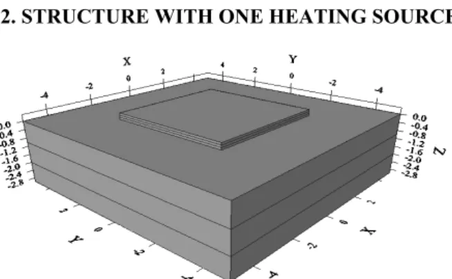
2. STRUCTURE WITH ONE HEATING SOURCE

Figure 1 –Structure of one heating source

The practical work begins by solving the thermal problem, and finding the steady state temperature of all chosen points (central point of each sub-layer). In this step, we use Rebeca-3D®, Flotherm® or any other 3D

thermal simulation software.

The procedure of calculating the thermal resistances Rth-3D

begins by calculating the value of Rth-3D for each

sub-layer by the following formula:

) 1 ( 1 3 _P T T RthD i i − − = (K°/W)

The second step is achieved by applying the equation that presents the relation between the temperature and the conductivity in the Rth-1D formula (in our case only Silicon

presents non-linear thermal characteristics). ) 2 ( ) 300 ( 68 . 154 ) ( 3 4 T T k_Si = (W/m.K°)

)

3

(

.

k

S

e

R

=

Wasim HABRA, Patrick TOUNSI, Jean Marie DORKEL

Transient Compact Modeling for Multi Chips Components

From (2) and (3) we get:

) 4 ( ) 300 ( ) 300 ( 68 . 154 . 4/3 4/3 1 1 T R T S e R D nonlinear D th Si Si th ₋ = =

Then, to transform the 1D non-linear equation to 3D one, we apply a correction coefficient given by the ratio between the Rth-1D and Rth-3D:

) 5 ( ) 300 ( . ) 300 ( 4/3 4/3 3 1 3 1 3 T R R R T R R D D D D nonlinear D th th th th th − = =

The final step is to introduce equation (5) in the expression of VCC (Voltage Controlled Current) control element, which can be found in ABM library of PSpice[4].

In order to enhance the nonlinearity phenomena by inducing a large temperature shift, we have made a simulation with a 250W of dissipated power and we got the next table of values:

Layer Rebeca-3D nonlinear aspect 1D-Rth Nonlinear _3D-R th Si1 97.571 (C°) 118.675 (C°) 97.701(C°) Si2 89.175 112.275 89.163 Si3 81.129 105.875 81.015 Cu1 73.369 99.475 73.174 Cu2 52.694 74.65 52.624 Cu3 37.486 49.825 37.475

Table1-Extracted temperatures by Rebeca-3D, compared with ones obtained by 1D and

3D-nonlinear CTMs

3. STRUCTURE WITH TWO HEATING SOURCES

When we apply a power on the first source, we can see that the generated isothermal surfaces take nearly the shape of half-sphere, one of them presents the temperature of the second source, which is inactive, and by applying the power on the second source we get the same effect (see Fig.2).

Figure2 - Illustration of OTCP.

The intersection between these two half-sphere is an arc that each point of it can present the thermal coupling between the two sources. The simplest is to choose the point that locates at the vertical central axis between the

two sources; this point is the Optimal Thermal Coupling Point (OTCP).

To illustrate in a practical example, we take the structure which is presented in fig.3, all this structure is made of Silicon in order to highlight the nonlinear properties of thermal conductivity.

Figure 3 –Structure with two heating sources.

Figure 4–illustration of the chosen point in the structure of two heating sources.

By applying the power on one of the two sources and launching the thermal simulation process with Rebeca-3D, we get the temperature of the points (A, B, C, and D). Because of the symmetry of structure, we can say that the value of thermal resistances between (A and B), (B and E) are the same as thermal resistances between (D and C), (C and E).

To calculate these thermal resistances we use the same formula as in the case of single source (1), so we get:

488 . 0 20 35 . 50 11 . 60 3 3 = − = = ₋ −B D C A D D R R (K°/W) 24585 . 1 20 433 . 25 35 . 50 3 3 = − = = ₋ −E C E B D D R R (K°/W) 02165 . 0 20 25 433 . 25 3 = − = −amb E D R (K°/W)

Finally, we apply the equation (5) in the expression of PSpice element (VCC). Fig.5 presents the corresponding CTM drawn in PSpice simulation software.

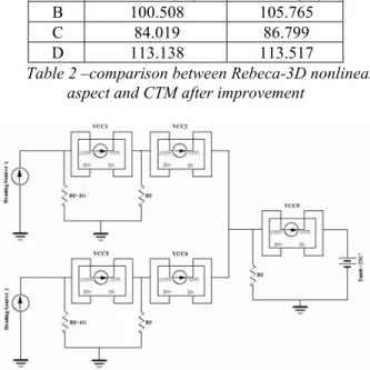
To validate our method, we launch a thermal simulation process by using Rebeca-3D with the nonlinearity aspect and dissipate a power of 40W on the first source and 50W on the second one, at the same time we launch the thermal simulation process on our compact model using P-Spice. Table2 presents the temperature for each point (A, B, C, and D) obtained from Rebeca-3d with nonlinear aspect, the 3D CTM, and the 3D-Nonlinear CTM.

Point Rebeca-3D 3D-Nonlinear A 139.722(C°) 142.27(C°) B 100.508 105.765 C 84.019 86.799 D 113.138 113.517

Table 2 –comparison between Rebeca-3D nonlinear aspect and CTM after improvement

Figure 5- The CTM for two heating sources

4. STRUCTURE WITH (MULTI) HEATING SOURCES

Fig.6 presents a simple structure with three heating sources and we will handle its CTM by the same way that has been followed with two heating sources.

Figure6 –Simple structure with three heating sources

So we launch the thermal simulation three times (because the asymmetrical structure), for each simulation, only one source dissipates 40W (fig.7). So we obtain from Rebca-3D the temperature of each source listed in table3:

Point Power on _Source1 Power on _Source2 Power on _Source3 Source1 101.346(C°) 25.538(C°) 25.375(C°) A 95.238 25.538 25.375 Source2 25.538 101.346 29.359 B 25.538 95.238 29.359 Sourc3 25.375 29.359 101.344 C 25.375 29.359 95.237

Table3 –The temperature of each point by Rebeca-3D

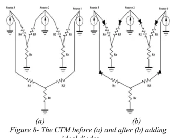
When we draw our model in p-Spice, we observe several important points:

1 - Because of the current of the sources 1, 2 and3 are divided into two branches (see fig. 7 and 8), the value of calculated Rth-3D have to be multiplied by (n-1) where n is

the number of the sources.

Figure7 –Illustration of the chosen points in case of three heating sources

2 - The calculations of the thermal resistances assume that: by applying a power on source 1, the temperature of X1 is the same as B, and X2is the same as C and so on (see fig.7). But in the electrical presentation of our CTM this principal is not valid because there is a current flow in the resistances R2, R4, R5 and R6 when we apply the power on source1 (see fig.8-a), so treating each two sources separately is not possible. To solve this problem, we add on each branch an ideal diode (fig.8-b) and so we can assure that the calculations of thermal resistances are valid for the electrical representation.

Wasim HABRA, Patrick TOUNSI, Jean Marie DORKEL

Transient Compact Modeling for Multi Chips Components

(a) (b)

Figure 8- The CTM before (a) and after (b) adding ideal diodes.

To validate what is explained above, we launch thermal simulation with Rebeca-3D, taking into account the non linear aspect. We apply on the first source 30W, on the second 40W, and on the third one 20W.

By applying the same dissipated power on our CTM and by dividing the resistances R1,R2, R3, R4,R5, and R6 successively into three resistances (to improve the model) we get the following table which presents the temperature of each source and the points A, B and C, obtained from Rebeca-3D and our 3D-Nonlinear CTM.

Point Rebeca-3D CTM Source 1 92.145(C°) 93.687(C°) A 86.176 87.701 Source 2 121.317 123.546 B 112.543 114.685 Source 3 72.719 70.58 C 69.002 66.921

Table4 – The comparison between Rebeca-3D nonlinear aspect and our 3D-Nonlinear CTM.

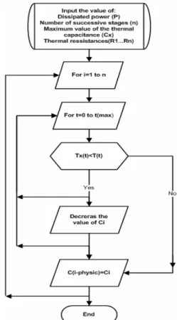
5. OPTIMIZING THE THERMAL CAPCITANCES

The optimization is based on the physical behavior that can be explained by:

- In the presented CTM (fig.9) we can say, with an accepted accuracy, that the only responsible capacitance for the curve changes of the transient response of junction until the temperature T1=P.R1

is C1, and for the changes until T2=P.(R1+R2) are

both C1 and C2, and so on….(where P is the

dissipated power).

- To make the optimization we have to begin by optimizing the value of C1 then C2 and so until the last thermal capacitance.

The benefits of the physical based optimization of the thermal capacitances are summarized by:

1- We are not forced to trace the transient response of several points; just the transient response of the junction is needed.

2- In the case of Multi chips model, it is difficult (practically) to find the physical localization of the thermal coupling points, and this method keep the physical presentation without going in the geometrical calculations.

3- The calculated capacitances are based on the values of the 3D thermal resistances, so they present 3D thermal capacitances.

Figure 9-Example for a transient CTM

(a)

(b)

(c)

Figure 10 -Transient response:

Figure 11- The flowchart of the thermal capacitances optimization

6. REFERENCES

[1] T. HAUCK, T. BOHM “Thermal RC Network Approach to Analyze Multi chip Power Packages”, SemiTherm Symposium 2000.

[2] H.I. Rosten, J.D. Parry, and others. “Final Report to SemiTherm XIII on the European-Funded Project DELPHI- the development of libraries and physical models for an integrated design environment”.13 IEEE- SemiTherm Symposium. [3] Ammous, H. Morel, B. Allard, and others. “Developing an equivalent thermal model for discrete semiconductor packages”. International journal of thermal sciences. VOL. 42 2003. [4] Application Note: “Analog Behavioral Modeling. Source: MicroSime Corporation Newsletter, Oct. 1989. Revised by: Tim CHRISTENSEN May 1999.