Therapeutic Magnetic Microcarriers Characterization by Measuring Magnetophoretic Attributes

(1)

UNIVERSITÉ DE MONTRÉAL

THERAPEUTIC MAGNETIC MICROCARRIERS CHARACTERIZATION BY

MEASURING MAGNETOPHORETIC ATTRIBUTES

GUILLERMO VIDAL IBACACHE

DÉPARTEMENT DE GÉNIE INFORMATIQUE ET GÉNIE LOGICIEL ÉCOLE POLYTECHNIQUE DE MONTRÉAL

MÉMOIRE PRÉSENTÉ EN VUE DE L’OBTENTION DU DIPLÔME DE MAÎTRISE ÈS SCIENCES APPLIQUÉES

(GÉNIE INFORMATIQUE) AOÛT 2013

(2)

UNIVERSITÉ DE MONTRÉAL

ÉCOLE POLYTECHNIQUE DE MONTRÉAL

Ce mémoire intitulé:

THERAPEUTIC MAGNETIC MICROCARRIERS CHARACTERIZATION BY MEASURING MAGNETOPHORETIC ATTRIBUTES

présenté par : VIDAL IBACACHE Guillermo

en vue de l’obtention du diplôme de : Maîtrise ès sciences appliquées a été dûment accepté par le jury d’examen constitué de :

M. LANGLOIS J.M. Pierre, Ph.D., président

M. MARTEL Sylvain, Ph.D., membre et directeur de recherche M. COHEN-ADAD Julien, Ph.D., membre

(3)

DEDICATION

(4)

ACKNOWLEDGEMENT

First of all, I appreciate the support that my research supervisor, Mr. Sylvain Martel, provided me during my journey in the NanoRobotics Laboratory. He was able to give me fresh insights when I went to him asking for advice. He is able to put the right questions in the right moment and to explain the more complex problems in very simple words, without his constant push and help this project would not have seen an end.

Working environment in the laboratory has been exceptional and, in my opinion, one of the major reasons for this is the presence of Mr. Charles Tremblay. He is energetic, joyful, an excellent professional, always willing to help and teach; and it is always a pleasure to talk to him on any subject.

Thanks to Ke Peng and Behnam Izadi, we spent a lot of time together setting up experiences that later were useful to do my own work. Ke is kind and warm, sharp-eyed and is always prompt to give help. Behnam is quiet, introverted, and hardworking; thanks to his work I was able to initially see the movement of aggregations in my experiments.

To Ms. Neila Kaou, who is always willing to listen and helped me with plans and some administrative stuff.

To Manuel Vonthron, head of the computer team who is always doing things really quickly and right with the enthusiasm of the youth. He is also always available to provide careful feedback.

To Viviane Lalande, who set a high bar to everyone in the lab with her excellent work and leadership.

To Alexander Bigot, talking to him is always a way to see the things with another prism, which is usually simpler than my tendency to complicate things.

To J.B. Mathieu, who spent a Saturday evening to explain to me how he was able to inject particles and did his incredible job with magnetic microparticles aggregations. He took time from his vacations to help me.

(5)

To Nina Olaemei, who helped me with the nightmare of trying to get a working microfluidic channel.

To all other members of the laboratory, who received me and were patient to my communication problems in English and especially in French.

Lastly, thanks to my family, my wife and kids that have been here all this time, dealing with my mood changes and supporting me with their love.

Porque no tenemos nada, queremos hacerlo todo...

- Carlos Dittborn

Alepue mapu küpan pian

amulen, amulen

alüpu puan

doy ayeple wanglen.

Vengo de las tierras de Alepue, diré

avanzo, avanzo

quiero llegar muy lejos

más allá del umbral de las estrellas.

(6)

ABSTRACT

Micro/nano robots are considered a promising approach to conduct minimally invasive interventions. We have proposed to embed magnetic nanoparticles in therapeutic or diagnostic agents in order to magnetically control them. A modified clinical Magnetic Resonance Imaging (MRI) scanner is used to provide the driving force that allows these magnetically embedded microcarriers to navigate the vascular human network. By using specific Magnetic Resonance (MR) gradient sequences this method has been validated in previous research works.

Magnetophoresis is the term used to describe the fact that a magnetic particle changes its trajectory under the influence of a magnetic force while being carried by a fluid flow. This movement depends on the particle’s magnetic characteristics, the particle’s geometric shape, the fluid flow’s attributes and other factors. In our proposed method, magnetic microcarriers can be produced in several different ways, and so their response will differ to the same magnetic force and fluid flow conditions. The outcome of the therapeutic treatment using our method depends on the adequate selection of the therapeutic and/or diagnosis agents to be used. The selected therapeutic and/or diagnosis magnetic microcarrier also influences the selection of the MR gradient sequence that best fit for a given treatment.

This master’s thesis presents the design of a device intended to assess the magnetophoretic properties of magnetic therapeutic microcarriers and/or diagnostic agents. Such characterization is essential for determining the optimal sequences of magnetic gradients to deflect their trajectory through relatively complex vascular networks in order to reach a pre-defined target. A microfluidic device was fabricated to validate the design. Magnetophoretic velocities are measured and a simple tracking method is proposed. The preliminary experimental results indicate that, despite some limitations, the proposed technique has the potential to be appropriate to characterize any drug and/or diagnosis magnetic microcarrier containing different magnetic nanoparticle content.

(7)

RÉSUMÉ

Des micro/nano-robots sont considérés comme une approche prometteuse pour mener des interventions minimalement invasives. Nous avons proposé d'intégrer des nanoparticules magnétiques dans des agents thérapeutiques ou de diagnostic afin de les contrôler magnétiquement. Un scanner d’imagerie par résonance magnétique (IRM) clinique modifié est utilisé afin de fournir la force motrice qui permet à ces microporteurs magnétiques à naviguer dans le réseau vasculaire humain. En utilisant des séquences spécifiques des gradients de résonance magnétique (MR) cette méthode a été validée dans des travaux de recherche antérieurs. Magnétophorèse est le terme utilisé pour décrire le fait qu'une particule magnétique modifie sa trajectoire sous l'influence d'une force magnétique tout en étant portée par un flux de fluide. Ce mouvement dépend des caractéristiques de la particule magnétique, de sa forme géométrique, des attributs de l'écoulement de fluide et d'autres facteurs. Dans notre méthode proposée, les microporteurs magnétiques peuvent être réalisés de différentes manières, et donc leur réponse sera différente à la même force magnétique et dans les mêmes conditions d'écoulement de fluide. Le résultat du traitement thérapeutique utilisant notre méthode dépend de la sélection adéquate des agents thérapeutiques et/ou de diagnostic à utiliser. Le microporteur magnétique thérapeutique et /ou de diagnostic choisi influe également sur le choix de la séquence des gradients magnétiques que meilleur se ajustement pour un traitement donné.

Ce mémoire de maîtrise présente la conception d'un dispositif destiné à évaluer les propriétés magnétophorétiques des agents microporteurs magnétiques thérapeutiques et/ou de diagnostic. Une telle caractérisation est essentielle pour déterminer les séquences optimales des gradients magnétiques pour dévier leur trajectoire à travers des réseaux vasculaires relativement complexes dans le but d'atteindre un objectif prédéfini. Un dispositif microfluidique est fabriqué pour valider la conception. Las vitesses magnétophorétiques sont mesurées et une méthode de suivi simple est proposée. Les résultats des experiences préliminaires indiquent que, malgré certaines limitations, la technique proposée a le potentiel d’être approprié pour caractériser n'importe quel microporteur magnétique thérapeutique et/ou de diagnostic contenant différents taux de nanoparticules magnétiques.

(8)

LIST OF TABLES

(12)

LIST OF FIGURES

Figure 2-1 CTV method schematics. Cells identified in the five consecutive frames are named t1

to t5 respectively. The search area between frames is determined by radius r. A predicted

location of the cell in frame 3 is indicated as p. The real cell path is depicted in green. ... 18 Figure 3-1 Schematic diagram of a general MRN procedure. ... 20 Figure 3-2 Free body diagram. Forces on a magnetic particle (green sphere in the center) in the

magnetophoretic chamber are depicted. The fluid flow is in x direction. Magnetic force is applied in y direction. In z direction acts gravity and buoyancy. Drag force resist movement in all directions. ... 21 Figure 3-3 Schematic representation of human cardiovascular system vessels. Vessels’ main

parameters depicted are inner diameter, average blood flow speed and Reynolds number adapted from [72]. ... 24 Figure 3-4 Bending problem in the initial chamber design. (a) Without magnetic steering force

applied. Magnetic microparticles are represented in blue. Stream-lines are represented by blue arrows crossing the chamber. The bending zone is indicated in the middle of the chamber. (b) Expected effect on a magnetic aggregation when the magnetic force is applied. The expected deflection trajectory is shown in red; the effect of the bending zone on deflection pattern is shown in green. ... 26 Figure 3-5 Schematics of fluid flow streamlines in channel connections. (a) Schematics of fluid

flow streamlines for right angle channel connection with vortex roll forming at the entrance of the magnetophoretic chamber (adapted from [16]). (b) Schematic of smoothed fluid flow by using angle connection. ... 27 Figure 3-6 Flow pattern in the magnetophoretic chamber. Flow observed in the magnetophoretic

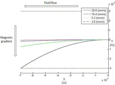
chamber when ink is pumped in the microparticles inlet and DI water in the main flow inlet. ... 29 Figure 3-7 Simulated individual microparticle’s deflection patterns. Flow velocities considered

(13)

Figure 3-8 Simulated microparticles aggregations deflection patterns. Flow velocities considered are 20.8, 10.4, 5.2 and 2.6 mm/s (from top to bottom in the graphic). ... 33 Figure 4-1 Schematic of the microfluidic device design. The complete device is 200 µm deep.

Magnetophoretic chamber is 7 mm × 6 mm. Main flow and microparticles flow meet in the 2 mm entrance channel. ... 44 Figure 4-2 Schematic of the experimental setup. Prop Coil 1 and Prop Coil 2 refer to the custom

Maxwell pair coils. It is seen that the fluid flow and magnetic gradient are intended to be orthogonal. Then all movement perpendicular to the flow is solely produced by the magnetic gradient from the propulsion coils. ... 46 Figure 4-3 Effect of the fluid flow velocity on the deflection pattern of magnetic microparticles

aggregations moving along the magnetophoretic chamber, in (a) the fluid velocity is 20.8 mm/s and it is difficult to notice the deflection of microparticles; in (b) the fluid velocity is 10.4 mm/s; in (c) fluid velocity is 5.2 mm/s, and in (d) it is set to 2.6 mm/s ... 46 Figure 4-4 Comparison between the tracking software applied to raw video (left side) and to

filtered frames video (right side). Only for the slower fluid velocity is possible to extract directly from raw video the trajectory of magnetic microparticle aggregations ... 47 Figure 5-1 Distance measurement to detect blob intersection. The quantities d1 = x2 - x1 and d2 =

y2 - y1 are horizontal and vertical distances between centroids of the blobs, w1, w2 are the

widths and h1, h2 are the heights of the blobs respectively. If d1 < (w1/2 + w2/2) ˄ d2 < (h1/2

+ h2/2) the blobs are considered merged. ... 52

Figure 5-2 Detected aggregations in different frames. Accumulated detected particles at different points in time are shown at left. Foreground resulted by background subtraction from current frame is shown at the right. The video used is the one at which the fluid velocity is 2.6 mm/s. Particles detected are highlighted with a circle surrounding them. ... 53 Figure 5-3 Filtering process example applied on the same frames as in Figure 5-2. The tracked

aggregation is highlighted by encircling it to show the effect of each filter step... 54 Figure 5-4 Window to enter fluid flow speed used in the opened video. ... 55 Figure 5-5 Spatial calibration. Selection of a region of known horizontal size that is used to

(14)

Figure 5-6 Tracking region selection. The user can define the region in which the tracking is to be

performed. ... 57

Figure 5-7 Simple flowchart of the preliminary tracking software. ... 58

Figure 5-8 Image processing prior to tracking. ... 59

Figure 5-9 Deflection pattern of aggregations in 2.6 mm/s movie. ... 62

Figure 5-10 Deflection pattern of aggregations in 5.2 mm/s movie. ... 62

Figure 6-1 Prolate ellipsoid representing magnetic chain-like aggregation shape. ... 66

Figure 6-2 Current chamber design problem. Aggregations represented in blue are subjected to the magnetic gradient at the right time. In green is represented the situation when the magnetic gradient is turned on too early. ... 68

(15)

LIST OF SYMBOLS AND ABBREVIATIONS

CTV Cell Tracking Velocimetry

DI De-ionized

HGMS High Gradient Magnetic Separation

MR Magnetic Resonance

MRI Magnetic Resonance Imaging MRN Magnetic Resonance Navigation MR-Sub Magnetic Resonance Submarine MRT Magnetic Resonance Targeting

MTTM Magnetophoretic Trajectory Tracking Magnetometry PMMA Polymethyl methacrylate

TMMC Therapeutic Magnetic Micro Carriers

(16)

LIST OF APPENDICES

(17)

CHAPTER 1 INTRODUCTION

1.1 Background and motivation

Minimally invasive interventions are attracting a lot of interest in the research community, mainly due to the advantages of this kind of interventions: reduced patient recovery time, shorter stay in the hospital and fewer complications. In the context of the Magnetic Resonance Submarine (MR-Sub) project a new minimally invasive technique for cancer treatment and diagnosis, called Magnetic Resonance Navigation (MRN), has been proposed. This technique is based on the use of the main magnetic homogeneous field and the magnetic gradients of an upgraded Magnetic Resonance Imaging (MRI) scanner in order to navigate therapeutic or diagnostic agents with embedded magnetic nanoparticles to target specific locations in the vascular human network.

Most of current cancer treatments involving drug administration are systemic, which means that the drugs are delivered in the bloodstream causing them to affect cells all over the organism with just around 1% or less destroying tumor cells [1, 2]. The MRN technique is expected to produce a significant increase in targeting efficiency and the feasibility of this method has already been demonstrated [3] by our research group.

A major challenge faced in this technique is the fact that the human vasculature is very complex and heterogeneous with vessels ranging from some millimeters (major arteries) to a few micrometers (arterioles, capillaries) in diameter. To accommodate the smaller human body vessels, the drug carrier size must be reduced, which in turn reduces the amount of drug that can be transported. On the other hand, smaller carriers are more difficult to be navigated due to its reduced magnetic volume.

In [4, 5] it was demonstrated that it is possible to produce a drug carrier of about 50 µm in diameter size to target a tumor deep inside the body. However, in [6] the authors noticed that normal MRI gradient coils were not sufficient to allow steering of magnetic microcarriers in a Y-shaped bifurcation, then upgraded gradient coils were tested and validated. In this last study it was also stated that, in order to improve steering efficiency, it could be exploited the fact that

(18)

magnetic microcarriers tend to agglomerate when being used as therapeutic and/or diagnosis vectors.

For improving targeting efficiency by using the aggregation of magnetic microcarriers we are obligated to understand and evaluate the response of these aggregations when subjected to magnetic gradients. In different given conditions of fluid flow and magnetic force, magnetic microparticle aggregations show different deflection patterns. Thus the study of this deflection patterns gives clues on the magnetic response of them. Hence, by evaluating deflection patterns the magnetophoretic velocity of these entities can be estimated and used to predict their behavior in treatment conditions.

Moreover, in [7] it has been published that even for magnetic microspheres of the same size prepared under the same conditions, magnetophoretic velocities can differ by a factor of 4 or more. This emphasizes the need for an instrument to estimate magnetic microcarriers response to magnetic gradients when designed to be used in targeted drug delivery and/or diagnosis applications in the context of MRN treatments.

1.2 Problem statement

The main goal of the MR-Sub project is to develop a platform capable of navigating magnetic microcarriers in the human cardiovascular system according to a pre-defined pathway.

1.2.1 Thesis objectives

The objective of this thesis is to design a device in order to collect data on the magnetic response of the microcarriers when used in MRN. To attain this objective the main goal is divided in the following sub-goals:

• design a microfluidic chamber in order to allow the magnetic microcarriers to move while following the fluid flow,

• record microparticles’ course when subjected to a magnetic steering force perpendicular to the direction of the flow.

(19)

• estimate the magnetophoretic velocity of magnetic particles, that in turn, should allow estimating the trajectory that a microcarrier would follow under similar circumstances.

Main contributions of the work for this thesis are:

• a conference paper presented in the 3M-NANO 2012 Conference (International Conference on Manipulation, Manufacturing and Measurement on the Nanoscale) in Xi’an, China under the title: “Characterization by magnetophoresis of therapeutic microcarriers relying on embedded nanoparticles to allow navigation in the vascular network” [70]; this work was selected as a Best Conference Paper Award Finalist.

• a journal paper published in 2013 in the Journal of Micro-Bio Robotics as: G. Vidal and S. Martel, "Measuring the magnetophoretic characteristics of magnetic agents for targeted diagnostic or therapeutic interventions in the vascular network" [10] .

• a microfluidics chamber design for magnetophoretic experiences.

• a basic software tracking tool tailored for the conditions of the magnetophoretic experiences performed.

Unless the contrary is indicated, the developments presented in this document are the contribution of the author. Exceptions are indicated and mainly are: OpenCV blobtrack modified application that was adapted by Behnam Izadi for experiences in Ke Peng’s master thesis work [8] and Joerg Buchholz’s Particle System Toolbox [9] used for magnetic microparticles movement simulations.

1.3 Overview of the thesis

The thesis organization is as follows: in the first chapter the background, motivation and problem statement are presented; in Chapter 2 there is a literature review on the way in which the trajectory of magnetic particles has been studied before and its previous applications; in Chapter 3 the approach used in this work is presented; in Chapter 4 the published paper [10] showing the preliminary results of the selected design in its original version is introduced; Chapter 5 introduces the proposed tracking method based on finding presented in Chapter 4; Chapter 6

(20)

presents a general discussion of this work; finally Chapter 7 summarizes the project and presents future perspectives for it.

(21)

CHAPTER 2 LITERATURE REVIEW

Retrieving data on the reactivity shown by MR navigable microcarriers seems to be fundamental in order to determine optimal control sequences during MRN treatments. This chapter focuses on providing an overview of previous work on the techniques for observing magnetic microparticles' trajectories, on the importance of aggregations in the context of MRN and the need for a method to estimate compared drug/diagnosis magnetic microcarriers performance. On the basis of this review the main advances in the area are highlighted.

2.1 Magnetophoresis

The study of the movement of magnetic particles in a fluid induced by the influence of a magnetic field (termed as magnetophoresis) has been the object of research in several works. As early as in 1960, an apparatus was proposed to measure the magnetic susceptibility of single particles by determining the velocity that particles get when in an inhomogeneous magnetic field [11]. This apparatus used a microscope to observe a particle’s trajectory and a stop watch to time the movement and then estimate the particle’s assumed velocity.

2.1.1 Magnetism basic concepts

In order to understand magnetophoresis, some basic definitions on magnetism in materials are required.

The magnetic induction, B1, is the response of a given material to an applied magnetic field, H. The relationship between B and H is given by (in SI units):

=

μ ( + )

2-1

1_{In this document bold letters indicate vectors : for example A is a vector and A is a scalar indicating the magnitude}

(22)

where µ0 is the permeability in free space and M is the magnetization induced inside the material

and is dependent on the characteristics of it. The magnetization is defined as the magnetic moment per unit volume

=

2-2

where m is the dipole magnetic moment and V is the volume of the magnetic material. The magnetic moment relates to the torque that is exerted on a magnet dipole or a current loop when a magnetic field is applied. The dipole magnetic moment of a material depends mainly on orbital and spin magnetic moments of the electrons in the constituent atoms of it.

The magnetic susceptibility of a material is defined by

=

2-3 The susceptibility is an indication of the responsiveness of a material to an applied magnetic field. Magnetization curves are built by plotting M versus H (or B versus H), and are used to identify the magnetic type of material.

The magnetic permeability is defined by

μ =

2-4

and indicates how permeable a material is to the applied magnetic field. Permeability µ and susceptibility χ (in SI units) are related by

μ = μ (1 + )

2-5 with µ0 the permeability in free space.

Materials are classified as diamagnetic, paramagnetic, antiferromagnetic, ferrimagnetic and ferromagnetic depending on their magnetic characteristics. For diamagnetic, paramagnetic and antiferromagnetic materials, magnetization curves are linear; a relatively large applied field is required to produce changes in magnetization and there is no remanent magnetization if the applied field is removed. For ferrimagnetic and ferromagnetic materials, magnetization curves have the typical hysteresis loop form; there is a magnetization saturation point after which

(23)

negligible change is produced in magnetization by increasing the applied field and removing the applied field does not reduce magnetization to zero (if saturation has been reached), this remanent magnetization has several technological applications [12].

2.1.2 Magnetic force

When an inhomogeneous magnetic field is applied to a particle, this magnetic field exerts a force on the particle given by:

= (

∙ )

2-6 where m is the dipole magnetic moment and

∇

B is the external magnetic field gradient. By using Eq. 2-2, we obtain the usual magnetic force expression used in this work:

=

( ∙ )

2-7 where Vf is the volume of the magnetic content [13].

On the other hand, in order to obtain magnetic susceptibility data from magnetophoretic experiments, it is usual to assume that the magnetic induction B and the magnetic applied field H are just related by permeability in free space, neglecting the effect of the magnetization M:

= μ

2-8 By combining Eq. 2-3 and Eq. 2-8 we obtain:

=

_μ

0 2-9

Then Eq. 2-7 becomes:

=

_μ

0

( ∙ )

2-10

Additionally as the moving particle displaces a fluid volume, it is also usual to take into account the magnetic force exerted on the medium, which leads to:

= −

_μ

(24)

with χm the susceptibility of the fluid medium, and the minus sign indicates that this force is

opposed to Fmag. Then, the usual expression for the net force on a magnetic particle exerted by a

magnetic inhomogeneous field is expressed in terms of the difference in susceptibility between the particle and the fluid:

=

_μ

0

( ∙ )

2-12

with ∆χ = χ - χm.

Finally, by applying a mathematical identity2 and the fact that there are no electric currents involved in the discussed setup, we obtain:

=

(

_2μ

2

0

)

2-13

which is the other usual form encountered in articles related to magnetophoresis [13, 14, 15]. It is commonly supposed that the inhomogeneous magnetic field varies only in one of the coordinate axes, then the magnitude of the force can be written as:

!"# $

=

%(

&

2

2μ

₀

)

2-14

where the operator ∇ is the standard derivative in the selected direction and B is the magnitude of the magnetic field in that direction.

2.1.3 Microfluidics basics

A microfluidics is a device that deals with fluid flow in channels with at least one dimension between 1 mm to 1 µm. When at least one of the dimensions of the channel is less than 1 µm, it is called nanofluidics.

Among the main advantages of microfluidics are: small sample quantities needed, high portability, fast and reliable results, and easy fluid control is possible.

2 _{( ∙ ) = 2 × ( × ) + 2( ∙ ) , as there are no electric currents}_∇∇∇∇

(25)

Fluid flows are characterized by the Reynolds number, a dimensionless parameter defined as:

'(

=

)

*+,-

_/

.

2-15 where Uflow is the average velocity of the flow, L is the characteristic or most relevant length

scale and ν is the kinematic viscosity of the fluid (defined as the dynamic viscosity µ divided by the density of the fluid ρ). This parameter describes the ratio between inertial and viscous forces in a fluid. The characteristic length L in channels is the hydraulic diameter Dh defined by:

1

2

=

44 ₅

2-16 with A the channel’s cross-sectional area and P the channel’s wetted perimeter.

Dimensions in microfluidics are small, which means that the Reynolds number is usually low, typically much less than 2100. This means that in microfluidics the flow regime is commonly considered as laminar flow. In this case, most flow patterns are simple, and are even expected to closely follow the geometry of the microfluidic channel [16].

When a rigid sphere moves in a microchannel and the Reynolds number for it is very low, the Stokes drag force formula is used:

67

= −69:;<

2-17 where r is the radius of the sphere, µ is the viscosity of the fluid and U is the microparticle’s velocity.

By using Eq. 2-16 and Eq. 2-12 (or Eq. 2-13), and considering steady-state (no acceleration, i.e., drag and magnetic forces balance) it is possible to obtain an estimate of the magnetic susceptibility of magnetic microparticles by measuring their magnetophoretic velocity.

2.1.4 Magnetophoretic trajectory observation

Video imaging based analysis of particles trajectory was proposed in [17] to determine the magnetic susceptibility of large numbers of individual particles. This study utilized particle tracking velocimetry (PTV) on videotaped sequences. PTV is a technique intended to analyze complex fluid fields by tracking individual seeds circulating with the fluid. This technique was

(26)

first proposed with this name in [18]. In [19] the PTV’s most recent algorithm version at the time is used. As PTV function is to visualize the fluid, particles are not individualized through the sequence of frames, which is a drawback in the proposed technique.

In [19, 20, 21] an instrument named as cell tracking velocimetry (CTV) was proposed for allowing the determination of the velocity of labeled cells and paramagnetic particles simultaneously by using microscopic video imaging and a computer algorithm, in a well-characterized magnetic energy gradient. The CTV had the objective of providing better insights for the outcomes to be expected in the magnetic cell separation process. The CTV is based on PTV, mainly solving the problem of particle’s identification through video frames. CTV has been also used to investigate magnetophoretic mobility changes produced in human blood cells by some infections [22].

In the context of drug delivery mediated by the use of treatment vectors with embedded magnetic particles, an optical method to measure the magnetic response, in some way a simplified CTV setup, is proposed in [23]. The main differences with the CTV technique are a reduced setup size, and the use of a commercial program for particle tracking and video acquisition (CTV used videotaped sequences).

Recently a method called magnetophoretic trajectory tracking magnetometry (MTTM) has been presented [24] with the aim of measuring a quantity defined as relative specific magnetic susceptibility by fitting the particle's observed trajectories with theoretical curves. The main difference of this method with CTV is the fact that particle's recorded trajectories are long compared with particle size.

All techniques presented hitherto study magnetic particles or cells in a still fluid. A technique referred as magnetophoretic velocimetry was proposed in [25, 26, 27, 28] to determine paramagnetic species adsorbed by single droplets through the analysis of the acquired magnetophoretic velocity under a high gradient magnetic field. The magnetic susceptibility of the droplets was expected to change according to the adsorption and be reflected by a change in their magnetophoretic velocity. In this technique the capillary contains a fluid that is moving and the migration of species is observed as a deviation from the fluid flow acquired speed.

(27)

Magnetophoretic velocity measurements were also exploited to evaluate the particle uptake in magnetic labeling of cells [29, 30, 31]; in [7] the measured magnetophoretic velocity of magnetically coated microspheres roughly scaled with the surface area.

2.2 Magnetic Manipulation

Basic magnetic manipulation of particles in microfluidics is classified, according to Gijs [32], in:

• Retention and separation: usually magnetic particles are immobilized by using a magnet, the magnetic material is separated from the solution in this way and can be analyzed a posteriori. Several other alternatives exist, for example continuous flow separation by Pamme’s group [39].

• Magnetic transport: In this approach, instead of deflecting the particles’ trajectory while moving with flow, magnetic particles move because of the action of magnetic actuation. This kind of manipulation is difficult due to the particles’ usual reduced magnetic volume.

• Magnetic labeling for detection: In this case, a magnetic label is attached to an entity of interest, and then detection devices are used to measure the produced magnetic field.

• Bead-flow interaction and mixing: magnetic particles tend to form chain-like aggregates due to dipole-dipole interactions. These aggregates can be used as plugs in certain applications, and by dynamically manipulating magnetic aggregations fluid mixing is possible in others.

One possible application of magnetophoresis is magnetic manipulation of magnetic particles as in separation, sorting and capture [15, 33]. For example, high gradient magnetic separation (HGMS) systems are used [34, 35, 36] to remove magnetic particles from a fluid flow. HGMS consists basically of a matrix of ferromagnetic material (wires or filaments) that captures magnetic particles as fluid flow passes through it while a high magnetic field is applied. After filtration has finished, the magnetic material is washed out as the magnetic field is turned off. The advantage of HGMS, to previous techniques of magnetic separation, is that allowed the trapping of relatively weak magnetic particles, which makes it suitable for biological applications [15].

(28)

As described in [37, 38], the relationship between magnetic manipulation and microfluidics is relatively recent. Pamme's group has developed a technique called free-flow magnetophoresis, a form of continuous flow separation that uses magnetic force to deflect the entities of interest [39, 40, 41, 42]. In this technique, magnetic particles are decoupled and deviated from their initial movement in a specific region of a magnetophoretic chamber. By these means, magnetic labeled particles exit the chip at specific positions depending on their magnetic properties. These outputs, with magnetic particles separated and sorted, can be used as inputs for other stages in more complex microfluidics applications. It is a continuous flow technique because magnetic particles are not trapped at certain regions of the microfluidics as in most other retention-separation methods. On the other hand, Furlani’s group has focused in developing models for predicting magnetic separation in different microfluidics systems and applications [43, 44, 45, 46].

In [47] a microfluidic device was designed for magnetic bead immunoassays. The main focus in this work is to automate as much as possible the assay by incubating the microparticles in the reagent while in continuous flow. The microparticles are moved from sample flow to reagent flow by using a magnetic translational force.

Examples as the above ones show the potential use of the magnetophoresis jointly with microfluidics to manipulate magnetic or magnetically functionalized particles.

2.3 Magnetic Resonance Navigation

The concept of MRN (Magnetic Resonance Navigation) is defined in [48] and it can be summarized as a method in which magnetically loaded therapeutic/diagnosis microcarriers are propelled and navigated by using gradient magnetic fields while inside the bore of an MRI scanner. In the first attempts to use MRN, the gradient magnetic forces were produced by the standard imaging coils of a MRI scanner. Since these initial experiences with MRN using millimetric sized cores as proof of concept [3, 49, 50], it was clear that magnetic propulsion forces produced by imaging coils of a standard MRI scanner were not suitable to navigate micro/nano sized carriers. In [51] it was shown that to perform navigation of micron sized agents in the form of a suspension, the use of enhanced magnetic gradient coils is needed and it was clear that the magnetic aggregation between particles due to dipole-dipole interaction could influence targeting efficiency. In [6, 52] aggregations were studied more deeply and it was

(29)

suggested that, due to its increased magnetic volume, they could be used to compensate the reduction of the propulsion force acting on individual magnetic particles.

The potential use of magnetic aggregation to improve therapeutic effectiveness has been pondered by research groups that intend to use MRN for other applications. The use of MRN for lung treatment by using aerosol drug delivery was explored in [53]; they conclude that the use of magnetic agglomerations is needed in order to allow the navigation of magnetic loaded aerosol drugs in the lungs. The size of the agents used in lung treatment means that enhanced gradient coils, as those proposed in [51], are not able to generate the forces needed to steer the magnetic agents. Then, the only way to overcome this problem is by exploiting magnetic agglomerations. In other studies, they proposed a detailed mathematical model [54, 55] for the forces involved in the magnetic aggregation process. The expected advantage of this theoretical framework is the possibility for assessing the steering efficiency without the need of performing actual experiments. They compared simulation results with the experiences performed in [6], and they argued that the simulation framework agreed with experiences. However they get 100% efficiency in the same situation as the experiences, but in the experimental setup it was not observed. On the other hand due to the non-slip boundary condition, they expected 0% efficiency when needle-like aggregations were parallel to the main flow, which seems unlikely.

Another possible application for MRN is the cell transplantation therapy. In [56] it was shown that MRN could be suitable for cell transplantation therapies, and in [57] the effect of magnetic cell aggregation was studied as an important factor to increase targeting efficiency. The improvement in targeting efficiency was attributed to the fact that cell aggregations show a higher magnetophoretic velocity.

In the context of MRN, all the presented works concluded that the steering ratio could be enhanced by exploiting magnetic aggregation. On the other hand, therapeutic agents are expected to be synthesized in several ways depending on their expected usage. For example, some could contain higher quantities of embedded magnetic nanoparticles while other could contain more therapeutic drug. This diversity is expected to play a role also in the therapeutic agents’ response to the exerted magnetic force produced by the gradient coils. For example, in [7] it was found that magnetic microspheres of the same size, prepared under similar conditions, presented magnetophoretic velocities differing by up to a factor of 4. Each one of the different therapeutic

(30)

agents could produce magnetic aggregations differing in size, stiffness, geometry, etc., and, therefore, behave differently in similar flow conditions and under the influence of the same magnetic gradient field. Moreover, in real treatment circumstances, physiological parameters could change unexpectedly. Additionally, in MRN fluid flow velocities are the ones found in human vascularity, which are relatively high when compared with fluid flow in experimental conditions in other applications.

To the best of our knowledge, there have been no other attempts to experimentally measure the trajectory of magnetic microcarriers in the context of MRN. In CTV and similar studies, there was no fluid flow involved; vertical and horizontal movements are due to gravity and magnetic force, respectively. The magnetic gradient was usually produced by a magnetic dipole, while in MRN it is produced by enhanced magnetic gradient coils. Finally, in our experimental conditions the magnetic micro-entities are inside the bore of a MRI scanner, therefore they are magnetized by the MRI’s magnetic homogeneous field, and there are dipole-dipole interactions between them. All of these conditions justify the design of a magnetophoretic testbench to study the trajectories of magnetic microcarriers to be used for MRN treatments in order to quantify their response to a given magnetic gradient in terms of their deflection patterns.

2.4 Object tracking

Observation of magnetic microcarriers’ trajectory means that software for their detection and tracking is needed. Object tracking has been the subject of a large amount of studies in computer vision and image processing [58] and has applications in many different areas as biology [59] and video surveillance [60]. The tracking problem can be defined as the survey of the movement that an object (or objects) follows in a sequence of frames of a video.

The first question to answer in this kind of application is to define the object to track. The answer to this question constitutes the way in which the object of interest is to be detected and represented. According to [58], the main object detection mechanisms are point detectors, background subtraction, segmentation, and supervised learning. In point detectors the aim is to find points in the object that are invariant to changes in illumination and camera viewpoint. Background subtraction uses a model for the static background and moving objects are frame regions that differ from this stationary background model (pixels that deviate from the

(31)

background model are marked for processing and are labeled as foreground pixels). Segmentation divides the image in partitions with similar characteristics. Finally, in supervised learning a training set is used to provide a model of the object to be detected. Once the object has been detected there are many ways of representing it, for example using geometric shapes, contours, points, etc. Usually this depends on the characteristics of the object being tracked. For example, for using in confocal microscopy, recently a new method for particle detection has been presented in [61] by exploiting radial symmetry of particles about its center. Particles' centers are located and represented as points. The algorithm determines the point of maximal radial symmetry by calculating the intensity gradient that it is expected to point towards the origins (particles’ centers).

The next step in object tracking is to define the way in which the features selected representing the object are going to be located in the next frame given its position in the previous one. In this case, a displacement model is needed in order to define a search area. Some popular models used are deterministic translational model [62] and Kalman filter method that uses the state space approach. It is intended to deal with noise and random perturbations that usually occur in real video data [58].

Finally, once the search area has been determined, it is needed to locate the object in it and a matching criterion is needed. One of the most common matching criteria is template matching in which a representative instance (template) of the object is defined in previous frames, then this template is compared within defined search regions in the current frame by evaluating similarity functions. This approach is usually a brute force method, exhaustive in nature. Another common matching criterion is the brightness constancy used in optical flow that is based in the assumption that corresponding pixels in consecutive frames have no brightness change [58].

As pointed out in [59], it seems that automatic tracking results are still rarely perfect and experimental conditions usually produce problems to tracking tools in most of the cases, due to the fact that these applications are usually tightly linked to their specific application.

(32)

2.4.1 Particle Tracking

Object tracking applied to motion of particles uses several specific approaches and the literature on the subject is extensive. Only some algorithms used in particle tracking that are of interest for this project are presented here.

Micro Particle Image Velocimetry (µPIV): this technique is an adaptation of the Particle Image Velocimetry (PIV) technique for use in microfluidics. It was introduced by Santiago et al [63]. PIV techniques are intended to measure instantaneous fluid velocities. Usually fluorescent particles are seeded into the fluid flow and the particles’ displacement is evaluated by image treatment techniques.

The typical PIV algorithm uses correlation to evaluate particles’ displacement. Frames are divided into areas; these areas are called interrogation areas or windows. Mathematical correlation calculation gives a measurement of similarity between interrogation windows. The Fast Fourier Transform (FFT) is often used to obtain the correlation, then the peak location is estimated and the displacement is derived.

Correlation is usually calculated by using cross-correlation, but auto-correlation has also been used. In auto-correlation one frame contains a double exposure recording. The drawback with auto-correlation is that flow direction must be known prior to apply it, because it results in more than one correlation peaks (typically three). In cross-correlation method, each exposure corresponds to an individual frame, the correlation calculation results in a single correlation peak that contains velocity information [64].

Particle Tracking Velocimetry (PTV): the aim of this method is mainly the one of the PIV. The main difference is that in this technique few particles are tracked, compared with high particle densities used in PIV. In fact, is often called low-image-density PIV.

In PTV, seeded particles are identified and tracked in the frame sequence. As mentioned before, one of the first introductions of PTV is done in [18]. A typical PTV algorithm consists of two main steps: particle identification to locate particles in a given frame and matching algorithm to evaluate the position of the identified particle at different times. Most of the research effort for this method has focused on improving the matching feature algorithm used to track particles in frame sequences.

(33)

Some of the best known PTV matching methods are: nearest-neighbor search with geometrical constraints, cross correlation between two frames, relaxation methods that analyze the probability of particle matching and genetic algorithms [65].

Computer vision designed techniques have been adapted for PTV. For example, Ruhnau et al. [65] use optical flow to track particles, and recently in [66] a computer vision based approach has been proposed to deal with particles’ overlapping problem in frame sequences.

Cell Tracking Velocimetry (CTV): this technique is a modified version of the PTV method used and developed in the Ohio State University [19]. This technique uses an image enhancement step prior to identification and tracking stages. The image enhancement steps are: histogramming used to find the range of the gray level present in the image, stretching used to improve contrast between particles and background, low-pass spatial filtering to remove noise, background subtraction and a final filtering step based on patterns to reconstruct incomplete cell images.

After image enhancement, the cell tracking algorithm is applied. This algorithm has two steps. The first step is cell location, which is based on a threshold level comparison to deduce if a given pixel is part of a particle (higher intensity than the threshold) or not. Once particles are located, a tracking module is used to establish the most probable path by using a sequence of five frames. The concept of path coherence is used to determine the particles’ paths. This concept supposes that object trajectory should be smooth. In Figure 2-1 the method is shown; cells positions for each of the five consecutive frames are t1, t2, t3, t4 and t5. Using the cell position in

the first frame (t1) as center, a search area is determined by radius “r” in the second frame. The

determination of this radius depends on several considerations, usually ranges between 1 to 3 times the cell diameter. Once the position in the second frame (t2) is established, the direction of

movement and distance between them can be established (red line). From this information the location of the cell in the next frame is predicted (cell tagged as “p” near to t3 in this example).

The error between real and predicted locations is used in a penalty function used to determine path coherence; the smaller the value of the penalty function, the greater the path coherence. The penalty function is used when more than one cell is identified in the search area of the next frame; the path with the smallest penalty function value is selected as the correct path. The procedure is repeated for frames 4 and 5. Finally the process is reversed, that is, the analysis is

(34)

done starting with frame 5 and ending with frame 1. If penalty function values have large differences in forward and reverse directions, then the paths are defined as not reliable [67].

Figure 2-1 CTV method schematics. Cells identified in the five consecutive frames are named t1 to t5 respectively. The search area between frames is

determined by radius r. A predicted location of the cell in frame 3 is indicated as p. The real cell path is depicted in green.

A multiple-frame PTV approach has been recently presented [68]. The main modification focuses in the way in which the prediction of particle position and velocity estimate is used to determine the radius of the search area in the next frame. It is expected that this method would improve the robustness and accuracy of PTV for highly seeded flows.

To summarize, to our best knowledge, the techniques to track moving particles have been adapted from methods used to study fluid flow behavior. PIV technique is commonly intended to provide information on the average fluid flow velocity, and PTV technique identifies and tracks individual particles. Given a specific problem, particle tracking approaches have been developed tailored to the specificities of the experimental conditions.

(35)

CHAPTER 3 OVERVIEW OF THE APPROACH

The aim of this thesis is to design a testbench device to characterize the microcarriers to be used as therapeutic/diagnosis carriers in order to better predict targeting efficiency in MRN treatments. The general goal of the MR-Sub project is to develop a navigation method for medical microcarriers to target deep regions in the human body by using an upgraded MRI system. This method has been demonstrated in vitro and in vivo [3, 4, 51].

In his Ph.D. thesis, J.B. Mathieu investigated the methods for navigating several microparticles as carriers for cancer treatment [69], concluding that magnetic aggregation of microparticles modifies their response significantly, but they were not completely characterized. The current work tries to build an incremental step in this subject by following some of the suggestions in J.B. Mathieu’s work, focusing on the study of the deflection trajectories, i.e., magnetophoretic velocities of aggregations to allow a better treatment prediction.

In order to do so, first of all it was needed to develop a microfluidic device allowing measurements of magnetophoretic response of magnetic particles and aggregations. As exposed in the literature review, magnetophoresis has been used for sorting and separation purposes, then a microfluidic chamber inspired in these applications was designed and tested to record microparticle aggregation movements. This design was presented as a conference paper in [70]. This work is a proof of concept of the magnetophoretic chamber.

After having been able to record and estimate the magnetophoretic velocity of microparticle aggregations by hand, the paper presented in the next chapter addresses the problem of automatic data gathering. The main focus of the paper is to cover initial results using the sample application called blobtrack [71] from OpenCV for tracking of microparticle aggregations. The idea with this work is to explore improvements to the device and protocol designed and tested in [70]; and to provide the start point for the design of tracking software tailored for characterization of microcarriers intended to be used in MRN.

(36)

3.1 Microfluidic design

In order to understand the importance of the magnetophoretic velocity in the MRN it is necessary to return to physical features that make MRN possible. These physical features will guide the design decisions used to fabricate the microfluidics magnetophoretic chamber.

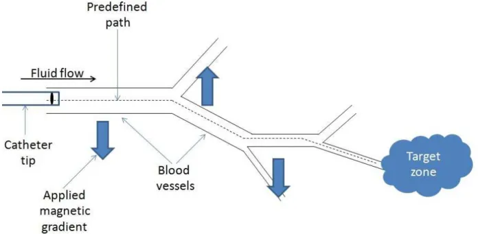
A general procedure in MRN can be summarized as follows: magnetic microcarriers are released in some predetermined point of the human vascular network (by using a catheter), then microcarriers are magnetically navigated through vessel bifurcations to reach the target location. The navigation is done following a predefined path. A schematic representation of a MRN procedure is shown in Figure 3-1.

Figure 3-1 Schematic diagram of a general MRN procedure.

3.1.1 Relevant physics principles

As has been discussed in the precedent section, the action force used in MRN is due to a controlled magnetic spatial variation and is given by (Eq. 2-7):

(37)

with M (A/m) the magnetization, and Vf (m3) the volume of the microcarrier’s magnetic content;

∇

B (T/m) is the magnetic gradient applied. Inside the bore of the MRI scanner there is a constant field denoted B0, usually big enough (1.5 T in the case of this project) to produce values close to

saturation magnetization in the microcarrier’s magnetic content.

Figure 3-2 Free body diagram. Forces on a magnetic particle (green sphere in the center) in the magnetophoretic chamber are depicted. The fluid flow is in x direction. Magnetic force is applied in y direction. In z direction acts gravity and buoyancy. Drag force resist movement in all directions.

Figure 3-2 gives a general outline of the involved forces when a microparticle is moving in fluid flow. By applying the Newton’s second law of motion we obtain that:

=

+

₆₇

+

₌

3-2 where m is the mass of the particle and a the acceleration, Fmag is the magnetic force applied in

the y axis, Fdrag is composed by Fdrag-x, Fdrag-y and Fdrag-z indicating fluid resistance to movement

in all directions, finally Fg is gravitational force and Fb is buoyancy. In the context of this work,

magnetic microparticles are supposed moving at the same speed of the fluid flow in the x axis, and then we consider that Fdrag-x is zero. On the other hand, movement along the z axis is usually

(38)

magnetic microparticle is large). Sedimentation is important because it causes the magnetic microparticles to touch the surface of the walls of the magnetophoretic chamber, and in that case, friction must be considered in the motion equation. The new simplified motion equation along the y axis is then:

=

+

₆₇ _> 3-3 By using the simplifications exposed above, the only involved forces are the magnetic and the drag force along the y axis. Moreover, when particles are moving in a fluid, an equilibrium state is reached such that the net force is zero (acceleration becomes zero).

0 =

+

₆₇ _>

3-4 When the Reynolds number is very low (much less than 1), we have mentioned that the drag force Fdrag-y is given by Stokes’ drag force formula (Eq. 2-17). At equilibrium the

magnetophoretic velocity is given by the balance between drag and magnetic forces, leading to:

=

67 >

= 69:;< =

( ∙ )

3-5 with µ the viscosity of the fluid, r the particle’s radius and U the speed of the particle with respect to the fluid flow. The volume of the magnetic content Vf is related to the particle’s radius r by:

=

?_@

9;

@_3-6 By solving Eq. 3-5 for speed and using Eq. 3-6, the particle’s magnetophoretic velocity is then given by:

<

=

2;2( ∙ )_9: 3-7 From Eq. 3-7 is clear that this magnetophoretic velocity can be adjusted by changing the size of the magnetic microcarrier (r2 term), by altering the magnetic gradient (∇∇∇∇B) or by

adjusting the magnetic magnetization (M) of the magnetic microcarrier.

This magnetophoretic velocity is a terminal steady velocity. It is important then to study the acceleration of the magnetic microcarrier as it approaches the steady-state to understand when it is possible to consider that the microcarrier has constant magnetophoretic velocity.

(39)

By using simplified relations in Eq. 3-5 and writing Eq. 3-3 in terms of the velocity we obtain the following expression:

BC

BD

=

( ∙ ) − 69:;C

3-8 assuming the magnetic force is applied only in the y direction, the solution to this equation is:

E(D) =

*_69:; F %&

G1 −

(

HIJKL M

N

3-9 in which

∇

is the derivative in the y axis; and M and B are the magnitudes of the magnetization and the inhomogeneous magnetic field.

From Eq. 3-9, the characteristic time scale in this situation is:

P =

_69:;

3-10 This characteristic time scale has been usually considered very small [16]. The assumption that the magnetophoretic velocity is the one given by Eq. 3-7 is safe in that case. However, when magnetic particle aggregations are being investigated, the size of the new “equivalent” microcarrier could increase the relaxation time due to Eq. 3-10 dependence on the mass of the new magnetic microcarriers aggregation.

3.1.2 Biological considerations

Blood flow velocity is usually very high in human vasculature. Common medium arteries in human are 2 mm to 6 mm in diameter, and flow velocities can range from 10 cm/s to 60 cm/s [72, 73, 74]. Figure 3-3 shows typical sizes and blood flow velocities in the human vascular system. In his work, Pouponneau et al. [5] used a bifurcation with a width of 2.5 mm to model a hepatic rabbit artery to test the feasibility of different ways to produce TMMCs to target liver cancer. In this work, it is also stated that the minimum size for microparticles used in liver embolization (in terms of their diameter) is 40 µm.

Due to the fact that Eq. 3-10 indicates that the relaxation time for this kind of experiments can be usually considered negligible, the magnetic microparticles and magnetic aggregations inside the magnetophoretic chamber are considered moving with the terminal magnetophoretic velocity when the magnetic gradient is applied.

(40)

Figure 3-3 Schematic representation of human cardiovascular system vessels. Vessels’ main parameters depicted are inner diameter, average blood flow speed and Reynolds number adapted from [72].

Based on the above information, the magnetophoretic chamber was designed to be 6 mm wide in order to simulate most of the distances that magnetic microcarriers are expected to cross. Plexiglas (PMMA) was selected as the material for fabricating the magnetophoretic chamber. Among its advantages one can mention low cost and high transparency (vital for magnetophoretic experiences) [75].

In MRN treatments, magnetic microcarriers are normally being injected in a vessel close to the targeted area by using a catheter. In [4] a catheter with a lumen3 of 0.7 mm (700 µm) is used to perform the experiments. This diameter was selected because it did not cause the magnetic microparticles aggregations to clog when the injection was performed. This information is used to decide the size of the channel that transports the magnetic microparticles into the magnetophoretic chamber. In order to allow similar conditions as the ones expected in real MRN experiences, the width of the entrance channel is selected as 500 µm.

In the same study [4], the designed TMMC particles are released between 20 and 30 mm from the bifurcation. In [76] the injection point in simulations is situated at 15 mm from the

(41)

bifurcation. This data is used to estimate that the magnetophoretic chamber should be about 15 to 20 mm long in order to emulate previously used experimental conditions.

As has been mentioned above, blood flow speeds for the sizes considered are quite large (between 10 cm/s to 60 cm/s). For a typical blood flow of 15 cm/s, the time to travel the expected 15 mm long chamber would be 10 ms. For a frame rate of 15 frames/s (which is the typical rate obtained with the MRI compatible camera), one frame is taken every 66 ms; then one could not be able to record the movement. In order to obtain 15 frames to analyze the deflection movement of a magnetic particle or a magnetic aggregation, 1500 frames/s would be needed. The video output signals of the MRI compatible camera are NTSC or PAL video signals, which gives a maximum of 30 frames/s (for NTSC). With this in mind, in order to obtain several frames to analyze deflection patterns, fluid flow speed must be reduced. Then in order to obtain at least 7 frames to analyze, the fluid flow should be no more than 30 mm/s.

3.1.3 Chamber

The initial chamber design was inspired by Pamme’s design used for continuous fluid flow separation [39]. In this design the magnetophoretic chamber is 6 mm by 6 mm with 16 plus 1 inlets of 100 µm wide evenly spaced and 16 outlets of 100 µm wide evenly spaced also, designed as a tree like succession of bifurcations. The chip is fabricated in glass, and the flow is produced by a syringe pump in withdrawal mode connected in the output. As pointed out before, the injection point in previous experiences was placed at 15 mm or more from the point of interest (bifurcation in this case). Then the design was modified to fit with the size of interest in our application. The number of inputs and outputs was reduced from 16 to 8 (plus the extra one in the input side).

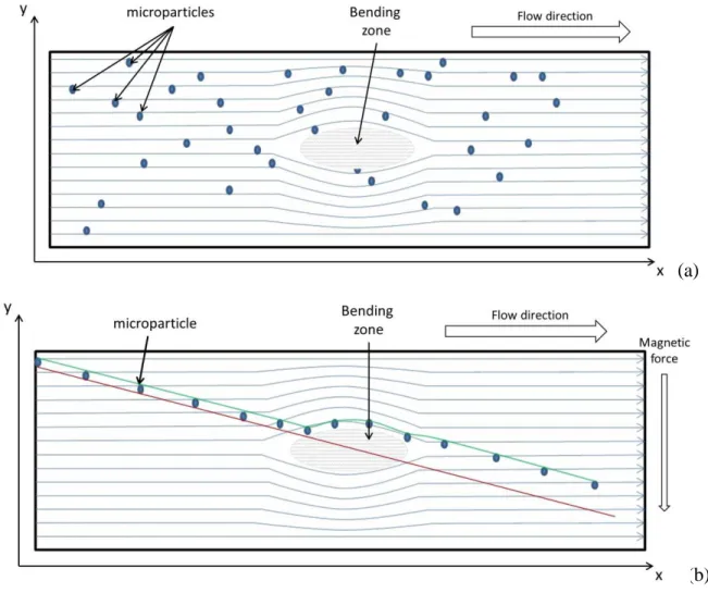
Because of the use of PMMA instead of glass and the chamber’s aspect ratio, the chamber was not at all functional due to deformations in the middle of the channel. Even using the pillars described in Pamme’s work [39], it was not possible to avoid this bending. In Figure 3-4 the deformation problem is schematically shown. Fluid flow moves in the x axis, the magnetic force is applied in the y axis and the deformation of the channel is in the z axis (not indicated). The resulting deformation in the z axis reduced the depth of the chamber in its center. In such a case, the fluid flow tended to move around the bending zone in the microfluidic chamber as depicted in

(42)

Figure 3-4. In addition, the negative pressure produced by the use of the syringe pump in withdrawal mode increased the bending effect in the center of the magnetophoretic chamber.

(a)

(b) Figure 3-4 Bending problem in the initial chamber design. (a) Without magnetic

steering force applied. Magnetic microparticles are represented in blue. Stream-lines are represented by blue arrows crossing the chamber. The bending zone is indicated in the middle of the chamber. (b) Expected effect on a magnetic aggregation when the magnetic force is applied. The expected deflection trajectory is shown in red; the effect of the bending zone on deflection pattern is shown in green.

Another difficulty found with this initial approach was the tree like design of the input and output channels. This design was supposed to evenly spread the fluid flow in the chamber. Initial

(43)

tests proved that this design decision was a problem in our case, mainly because of the air bubbles. In any symmetric bifurcation, any perturbation can destroy the symmetry of the flow. The air bubbles tended to clog the branches where they stay, avoiding the liquid to flow, and then perturbations were produced in the flow inside the chamber.

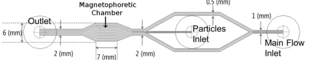
Based on these initial tests, the microfluidic design was modified to try to avoid as much as possible the problems found. The size of the magnetophoretic chamber area was reduced to 6 mm wide by 7 mm long. The microfluidic device is designed to measure and record microparticle trajectories, and not to collect them according to their magnetophoretic velocity. Accordingly, the input and output networks were transformed into single channels. The connection between input and output channels is performed in angle (Figure 3-5 (b)). The design is done taking into account that a right angle can produce turbulences in the fluid flow (Figure 3-5 (a)), and then the entrance and exit from the chamber are done in 45° in order to avoid this effect and obtain a smoother fluid flow (Figure 3-5 (b)).

Figure 3-5 Schematics of fluid flow streamlines in channel connections. (a) Schematics of fluid flow streamlines for right angle channel connection with vortex roll forming at the entrance of the magnetophoretic chamber (adapted from [16]). (b) Schematic of smoothed fluid flow by using angle connection.

Therapeutic Magnetic Microcarriers Characterization by Measuring Magnetophoretic Attributes