HAL Id: hal-00329218
https://hal.archives-ouvertes.fr/hal-00329218
Submitted on 1 Jan 2001
HAL is a multi-disciplinary open access
archive for the deposit and dissemination of
sci-entific research documents, whether they are
pub-lished or not. The documents may come from
teaching and research institutions in France or
abroad, or from public or private research centers.
L’archive ouverte pluridisciplinaire HAL, est
destinée au dépôt et à la diffusion de documents
scientifiques de niveau recherche, publiés ou non,
émanant des établissements d’enseignement et de
recherche français ou étrangers, des laboratoires
publics ou privés.
Coordinated Cluster and ground-based instrument
observations of transient changes in the magnetopause
boundary layer during an interval of predominantly
northward IMF: relation to reconnection pulses and
FTE signatures
M. Lockwood, A. Fazakerley, H. Opgenoorth, J. Moen, A. P. van Eyken, M.
Dunlop, J.-M. Bosqued, G. Lu, C. Cully, P. Eglitis, et al.
To cite this version:
M. Lockwood, A. Fazakerley, H. Opgenoorth, J. Moen, A. P. van Eyken, et al.. Coordinated
Clus-ter and ground-based instrument observations of transient changes in the magnetopause boundary
layer during an interval of predominantly northward IMF: relation to reconnection pulses and FTE
signatures. Annales Geophysicae, European Geosciences Union, 2001, 19 (10/12), pp.1613-1640.
�hal-00329218�
Annales Geophysicae (2001) 19: 1613–1640 c European Geophysical Society 2001
Annales
Geophysicae
Coordinated Cluster and ground-based instrument observations of
transient changes in the magnetopause boundary layer during an
interval of predominantly northward IMF: relation to reconnection
pulses and FTE signatures
M. Lockwood1, 2, A. Fazakerley3, H. Opgenoorth4, J. Moen5, 6, A. P. van Eyken7, M. Dunlop14, J.-M. Bosqued8, G. Lu9, C. Cully17, P. Eglitis4, I. W. McCrea1, M. A. Hapgood1, M. N. Wild1, R. Stamper1, W. Denig15, M. Taylor3, J. A. Wild10, G. Provan10, O. Amm11, K. Kauristie11, T. Pulkkinen11, A. Strømme12, P. Prikryl13, F. Pitout4,
A. Balogh14, H. R`eme8, R. Behlke4, T. Hansen12, R. Greenwald16, H. Frey21, S. K. Morley2, D. Alcayd´e8, P.-L. Blelly8, E. Donovan17, M. Engebretson18, M. Lester10, J. Watermann19, and M. F. Marcucci20
1Solar Terrestrial Physics Division, Department of Space Science and Technology, Rutherford Appleton Laboratory,
Oxfordshire, UK
2Department of Physics and Astronomy, Southampton University, Southampton, UK 3Mullard Space Science Laboratory, Holmbury St. Mary, Surrey, UK
4IRF, Swedish Institute of Space Physics, Uppsala Division, Sweden 5Department of Physics, University of Oslo, Blindern, Oslo, Norway
6Also at Arctic Geophysics, University Courses on Svalbard, Longyearbyen, Norway 7EISCAT Scientific Association, Longyearbyen, Svalbard, Norway
8CESR, Centre d’Etude Spatiale des Rayonnements, Toulouse, France
9High Altitude Observatory, National Center for Atmospheric Research, Boulder, Colorado, USA 10Department of Physics and Astonomy, Leicester University, Leicester, UK
11Finnish Meteorological Institute, Helsinki, Finland 12University of Tromsø, Tromsø, Norway
13Communications Research Centre, Ottawa, Ontario, Canada 14Blackett Laboratory, Imperial College, London, UK 15AFRL, Hanscom AFB, Cambridge, MA, USA
16Remote Sensing Group, Applied Physics Laboratory, John Hopkins University, Laurel, MD, USA 17University of Calgary, Calgary, Canada
18Department of Physics, Augsburg College, Minneapolis, MN, USA 19Danish Meteorological Institute, Kobenhavn, Denmark
20Istituto di Fisica dello Spazio Interplanetario – CNR, Rome, Italy 21Space Science Centre, Berkeley, USA
Received: 27 April 2001 – Revised: 11 July 2001 – Accepted: 16 July 2001
Abstract. We study a series of transient entries into the
low-latitude boundary layer (LLBL) of all four Cluster spacecraft during an outbound pass through the mid-afternoon magne-topause ([XGSM, YGSM, ZGSM] ≈ [2, 7, 9] RE). The events
take place during an interval of northward IMF, as seen in the data from the ACE satellite and lagged by a propagation delay of 75 min that is well-defined by two separate stud-ies: (1) the magnetospheric variations prior to the northward turning (Lockwood et al., 2001, this issue) and (2) the field clock angle seen by Cluster after it had emerged into the magnetosheath (Opgenoorth et al., 2001, this issue). With an additional lag of 16.5 min, the transient LLBL events
cor-Correspondence to: M. Lockwood ([email protected])
relate well with swings of the IMF clock angle (in GSM) to near 90◦. Most of this additional lag is explained by ground-based observations, which reveal signatures of transient re-connection in the pre-noon sector that then take 10–15 min to propagate eastward to 15 MLT, where they are observed by Cluster. The eastward phase speed of these signatures agrees very well with the motion deduced by the cross-correlation of the signatures seen on the four Cluster spacecraft. The evidence that these events are reconnection pulses includes: transient erosion of the noon 630 nm (cusp/cleft) aurora to lower latitudes; transient and travelling enhancements of the flow into the polar cap, imaged by the AMIE technique; and poleward-moving events moving into the polar cap, seen by the EISCAT Svalbard Radar (ESR). A pass of the
DMSP-1614 M. Lockwood et al.: Coordinated Cluster and ground-based instrument observations F15 satellite reveals that the open field lines near noon have
been opened for some time: the more recently opened field lines were found closer to dusk where the flow transient and the poleward-moving event intersected the satellite pass. The events at Cluster have ion and electron characteristics pre-dicted and observed by Lockwood and Hapgood (1998) for a Flux Transfer Event (FTE), with allowance for magneto-spheric ion reflection at Alfv´enic disturbances in the magne-topause reconnection layer. Like FTEs, the events are about 1 REin their direction of motion and show a rise in the
mag-netic field strength, but unlike FTEs, in general, they show no pressure excess in their core and hence, no characteristic bipolar signature in the boundary-normal component. How-ever, most of the events were observed when the magnetic field was southward, i.e. on the edge of the interior magnetic cusp, or when the field was parallel to the magnetic equa-torial plane. Only when the satellite begins to emerge from the exterior boundary (when the field was northward), do the events start to show a pressure excess in their core and the consequent bipolar signature. We identify the events as the first observations of FTEs at middle altitudes.
Key words. Magnetospheric physics (magnetopause, cusp
and boundary layers; magnetosphere-ionosphere interac-tions; solar wind-magnetosphere interactions)
1 Introduction
The low-latitude boundary layer (LLBL) is characterised by the presence of both magnetosheath and magnetospheric plasma inside the main magnetopause current sheet (Hones et al., 1972; Akasofu et al., 1973; Eastman et al., 1976; Haerendel et al., 1978; Eastman and Hones, 1979; Sonnerup, 1980; Sckopke et al., 1981; Mitchell et al., 1987; Hapgood and Bryant, 1990; Gosling et al., 1990a, b, c; Song et al., 1990; Sckopke, 1991; Traver et al., 1991; Fuselier et al., 1992; Woch and Lundin, 1993; Woch et al., 1993; Saun-ders, 1983; Hapgood and Lockwood, 1993, 1995; Phan et al., 1997; Savin et al., 1997; Fujimoto et al., 1998). The origin of this layer is one of the major unanswered questions in mag-netospheric physics and a key unknown in this regard is the topology of the LLBL field lines: it is interesting to note that roughly half of the papers cited above interpret the LLBL in terms of closed field lines, and the other half in terms of open field lines. There are three main classes of theory of LLBL formation (see review by Sibeck et al., 1999): (1) magne-tosheath plasma is injected by some process (such as wave-driven diffusion) onto closed field lines that are already popu-lated with magnetospheric plasma (Drakou, 1994; Lotko and Sonnerup, 1995; Treumann et al., 1991, 1995; Winske et al., 1995); (2) The plasma mixture arises on newly opened field lines along which magnetosheath plasma has flowed into the magnetosphere but magnetospheric plasma has yet to escape, either due to time-of-flight considerations (Lockwood and Smith, 1993; Onsager, 1994; Lockwood, 1997a, b; Fuselier et al., 1999; Onsager and Lockwood, 1997), or ion
reflec-tion at the reconnecreflec-tion layer Alfv´en waves (Cowley, 1982; Lockwood et al., 1996) or because a magnetic bottle still ex-ists on open field lines (Daly and Fritz, 1982; Scholer et al., 1982a; Cowley and Lewis, 1990; Lyons et al., 1994); (3) The field lines of the LLBL had been open, allowing for the mag-netosheath plasma to enter, but have subsequently been re-closed by re-reconnection (Nishida, 1989; Song and Russell, 1992; Song et al., 1994; Richard et al., 1994). In both (2) and (3), gradient and curvature drift across the open-closed boundary may sometimes help to replenish magnetospheric plasma that has been lost when it flowed across the magne-topause along open field lines.
1.1 Middle and low altitude signatures of the LLBL In addition to observations made at the magnetopause, data from mid- (Woch et al., 1993, 1994) and low- (Newell and Meng, 1988, 1992) altitudes have been used to discuss the LLBL. The “cleft” precipitation is often thought of as a the field-aligned projection of the LLBL (Vasyluinas, 1979; Newell and Meng, 1988; 1989, 1992, 1993, 1994a; Newell et al., 1991). However, this concept does not allow for two important considerations. First, the low-altitude observations are of particles that are within the loss cone and the magne-topause observations are of particles that are primarily out-side of the lost cone. Thus, the low-altitude observations of the LLBL require that the loss cone is filled and this need not be true of the magnetopause observations. Thus, for ex-ample, the mechanism proposed by Song and Russell (1992) will not yield a low-altitude LLBL (the filling of the loss cone with magnetosheath plasma ceasing when the field lines are re-closed), unless one also invokes strong pitch angle scat-tering of trapped particles on the re-closed field lines into the loss cone. Second, such field-line mapping does not al-low for the effects of velocity dispersion which is significant for ions in a convecting magnetosphere (Rosenbauer et al., 1975; Reiff et al., 1977). This dispersion does not allow for LLBL boundaries at high altitudes to be mapped to low alti-tudes whenever there is convective flow across that boundary (Lockwood and Smith, 1993). Since observations of dayside convection show flow into the polar cap throughout much of the dayside (e.g. Jorgensen et al., 1984), usually without a pronounced restriction or throat (Heelis et al., 1976), this ap-pears to be the case for a large fraction of the dayside. The open magnetosphere model predicts that the precipitation at low altitudes evolves in its classification from “LLBL/cleft” to “cusp” to “mantle” and then to “polar cap” as the field line evolves over the magnetopause away from the reconnection site and into the tail lobe (Cowley et al., 1991; Lockwood and Smith, 1993, 1994; Onsager et al., 1993; Lockwood, 1995). This evolution is seen in full along the flow streamlines in the steady state case and thus may sometimes be seen if the satel-lite follows the flow streamline quite closely (Onsager et al., 1993; Lockwood et al., 1994). Thus, several authors have ar-gued that much of the low-altitude LLBL precipitation must be on open field lines (Lockwood and Smith, 1993; Lyons et al., 1994; Moen et al., 1996; Fuselier et al., 1991, 1992,
M. Lockwood et al.: Coordinated Cluster and ground-based instrument observations 1615 1999). Other authors, while accepting that this is true when
reconnection is taking place, now argue that there is also a closed LLBL at low-altitudes nearer dawn and dusk (Newell and Meng, 1997). Lockwood (1997a) has shown how adopt-ing an open topology for the LLBL solves a number of long-standing anomalies.
The idea that the low-altitude signature of the LLBL is ion open field lines is supported by the fact that it covers roughly the same longitudinal extent as the low-altitude man-tle (Newell and Meng, 1992), which is known to also be on open field lines (Xu et al., 1995). The longitudinal extent of the cusp is lower than that of both the LLBL and the mantle (Aparicio et al., 1991; Newell and Meng, 1992) and would be set by the longitudinal variation of sheath plasma con-centration (Lockwood, 1997a). In addition, studies of the voltage across regions of low-altitude LLBL precipitation in both hemispheres (Lu et al., 1994) show that on any one flank (dawn or dusk), the same voltage does not always appear in the two hemispheres: we interpret this as indicating that at least some of the flank low-altitude LLBL was on open field lines and not closed field lines in these cases. Some obser-vations also show LLBL-like precipitation on sunward con-vecting field lines (Nishida et al., 1993; Nishida and Mukai, 1994). There is some debate as to whether these are truly LLBL field lines (Newell and Meng, 1994b) but the sun-ward convection can be explained in terms of the curvature force on open field lines but is inconsistent with mechanisms that transfer sheath plasma and momentum onto closed field lines.
1.2 The open LLBL at the magnetopause
Observations confirm the existence of an “open LLBL” (a term hereafter used for an LLBL on field lines that have an open topology) at the magnetopause. This type of LLBL is characterised by accelerated flows of magnetosheath-like ions. The evidence that they are injected and accelerated by flowing along newly-opened field lines includes: an observed dependence of the east-west flow direction on the IMF BY
component and hemisphere (Gosling et al., 1990a); results of tangential stress balance tests (Paschmann et al., 1979, 1986; Sonnerup et al., 1981, 1986; Johnstone et al., 1986); obser-vations of D-shaped distribution functions of injected ions (Smith and Rodgers, 1991; Fuselier et al., 1991; Gosling et al., 1990b, c) as predicted by Cowley (1982); the observa-tion of magnetosheath electron and ion edges inside the mag-netic field rotational discontinuity (Gosling et al., 1990c); and depleted populations of trapped particles (Scholer et al., 1982a; Daly and Fritz, 1982). The observations by Fuselier et al. (1991) show that the ion distributions on both sides of the magnetopause of both magnetospheric and magne-tosheath origin are as predicted by the theory of plasma mix-ing along open field lines. In addition, Smith and Rodgers (1991) applied the stress-balance test to show that the low-velocity cut-off of the injected sheath population was close to the local de-Hoffman Teller frame velocity, as also pre-dicted by the theory. Thus, at least part of the magnetopause
LLBL is formed by plasma mixing on field lines opened by magnetopause reconnection. Such processes could act for all IMF orientations, for example, a reconnection site at high-latitudes above the magnetic cusp, similar to the type studied by Gosling et al. (1991), has been seen to give rise to a day-side LLBL (Paschmann et al., 1990).
At this time we should clarify some semantic points about nomenclature. Some authors would not term an open field line region as an “LLBL” at all. Instead they would use the term “accelerated flows” or “reconnection layer”, as envis-aged by Levy et al. (1964), Heyn et al. (1988) and Lin and Lee (1993) and reserve the term LLBL for a layer on closed field lines. In addition, the open LLBL produced by lobe re-connection has also been referred to as an “overdraped lobe” (Crooker, 1992).
1.3 The closed LLBL at the magnetopause
Many researchers have discussed an LLBL on closed field lines (see review by Lotko and Sonnerup, 1995). Since the LLBL was found to generally flow faster away from the subsolar point (Haerendel et al., 1978), along with in-dications that it was also thinner at this point (Mitchell et al., 1987; Manuel and Samson, 1993), Eastman and Hones (1979) suggested that the LLBL was formed by the diffusion of magnetosheath plasma across the magnetopause. How-ever, Sonnerup (1980) pointed out that the observed waves were not adequate to drive the required diffusion, a finding confirmed by later studies (Owen and Slavin, 1992; LaBelle and Treumann, 1995; Winske et al., 1995; Treumann et al., 1995). Other mechanisms have been proposed for particle in-jection onto a closed LLBL, but they were found to be either invalid or inadequate. For example, one proposed impulsive penetration mechanism has been demonstrated to be theoret-ically unsound (Owen and Cowley, 1991).
Nishida (1989) proposed a mechanism whereby reconnec-tion may be responsible for plasma populareconnec-tions on a closed LLBL when the IMF points northward. He invoked highly patchy reconnection such that field lines opened at one re-connection site were re-closed a short time later elsewhere. During the time that the field line was open, magnetosheath plasma was free to flow in and magnetosphere plasma flowed out, thus releasing giving the observed plasma mixture which is trapped when the field line is closed again. More recently, Song and Russell (1992) and Song et al. (1994) proposed a similar mechanism, but used only two large-scale lobe re-connection sites poleward of the magnetic cusps. Numeri-cal simulations by Richard et al. (1994) indicate that magne-tosheath plasma may indeed move onto closed field lines in this manner during intervals of northward IMF.
1.4 “Subsolar” reconnection during northward IMF Another possibility is that low-latitude reconnection may of-ten be maintained during periods of northward IMF, as it is during southward IMF. The term “low-latitude” here means that the reconnection site is between the magnetic cusps such
1616 M. Lockwood et al.: Coordinated Cluster and ground-based instrument observations that it generates new open flux from closed flux. Studies of
transpolar voltage as a function of IMF orientation show that the rate of production of such LLBL field lines must be low during northward IMF (Reiff and Luhmann, 1986; Cowley, 1984; Freeman et al., 1993; Boyle et al., 1997). Neverthe-less, it may be sufficient to produce an open LLBL even dur-ing northward IMF, especially if the IMF clock angle θ IMF is not too small (typically > 45◦). Evidence for this comes from electron and ion distribution functions and flows in the LLBL (Onsager and Fuselier, 1994; Fuselier et al., 1995; Chandler et al., 1999). In addition, studies of the cusp au-rora during weakly northward IMF show evidence for contin-ued low-latitude reconnection, in addition to lobe reconnec-tion (Sandholt et al., 1996, 1998). Such reconnecreconnec-tion during northward IMF was also deduced by Nishida et al. (1998) from tail observations made by the GEOTAIL satellite. One possibility, suggested by Anderson et al. (1997), is that the magnetosheath field is distorted and amplified in the plasma depletion layer (which is less readily eroded during north-ward IMF) and this allows low-latitude reconnection to con-tinue even when the upstream IMF points northward. Recent work shows that if the IMF vector has a northward compo-nent, but lies at about 45◦of the magnetic equatorial plane (45 < θIMF < 90◦), the cusp/cleft aurora bifurcates into
two bands (Sandholt et al., 1996, 1998, 1999; Lockwood and Moen, 1999). The higher latitude part is consistent with the reconfiguration of “old” open flux by reconnection at the lobe magnetopause. There are two possible origins of the lower latitude band: it could be the signature of the loss cone refill-ing a closed northward-IMF LLBL, or it could be on newly opened field lines that are produced by continued sub-solar reconnection, despite the northward IMF component (proba-bly at a different MLT to the lobe reconnection site). McCrea et al. (2000) observed the equatorward erosion of the lower latitude band using EISCAT radar data and this argues for the reconnection origin and an open LLBL.
Hall et al. (1991) found that the counterstreaming elec-trons often used to define the LLBL (for example, Taka-hashi et al., 1991) are present most of the time on most of the dayside magnetopause. Lockwood and Hapgood (1997, 1998) have used the ion observations and tangential stress balance tests to show that the counterstreaming is well ex-plained as being a response of the electron gas to ion flight time effects, which is required to maintain quasi-neutrality on newly-opened field lines (Burch, 1985). The fact that these electron streams are seen during both southward and northward IMF therefore implies that reconnection is nearly always taking place somewhere on the magnetopause and is able to coat most of the boundary with newly-reconnected field lines and thus counterstreaming injected sheath elec-trons.
1.5 Distinguishing of open and closed models of the LLBL Making the distinction between open and closed field lines from observations of the LLBL is notoriously difficult, but has usually rested on the forms of the particle distribution
functions. It has been argued that particle distributions often used to classify field lines as closed, can arise simply in the open magnetosphere model. This does not necessarily mean that all of the LLBL is on open field lines, but it does im-ply that more of it may be than previously had been thought. In an open LLBL, the particle populations vary with time elapsed since the field line was reconnected. This means that any reconnection rate changes will result in spatial structure (“cusp ion steps”) in the open LLBL and cusp (Lockwood and Hapgood, 1997, 1998). This concept has been used suc-cessfully to explain spatially structured magnetosheath ion precipitation at lower altitudes (Lockwood and Smith, 1992, 1994; Lockwood and Davis, 1996; Lockwood et al., 1998).
There is a good reason to search for a unified mechanism for a particle injection into the LLBL and a single magnetic topology within the LLBL. Hapgood and Bryant (1992) have shown that electron temperature varies in a consistent and repeatable manner with electron density throughout nearly all magnetopause crossings. Fluctuations in the time series of both quantities are produced by magnetopause motions, but these are effectively caused by the satellite moving back and forth along what is a continuous transition in the bound-ary rest frame. Such a transition, seen in the moments of the electron gas, could be present for almost any process that causes mixing of the magnetospheric and magnetosheath populations. What is significant, however, is that using these electron data to indicate the satellite’s relative position in the LLBL (the “transition parameter”) reveals coherent structure in both the ion flows and magnetic field, which are inde-pendent of the electron measurements (Hapgood and Bryant, 1992; Hapgood and Lockwood, 1993). Recently, Lockwood and Hapgood (1997) have shown that the transition parame-ter (the degree of electron mixing) bears a simple relationship to time-elapsed since reconnection, showing that transition parameter works because there are open field lines coating the magnetospheric surface, i.e. an open LLBL. With this being the case, the most significant point is that the transi-tion parameter ordering is effective for nearly all passes in all parts of the LLBL, producing coherent variations through structures such as FTEs and accelerated flow events, as well as seemingly closed LLBL field lines (Hapgood and Lock-wood, 1995). It is difficult to see how the smooth coherent structure could be achieved by a variety of mechanisms.
The identification of closed LLBL field lines has usually rested on two features, namely trapped magnetospheric par-ticles and bi-directional streaming electrons.
1.6 Trapped particles
Trapped particles with a double loss cone pitch-angle dis-tributions arise on closed field lines connecting both iono-spheres. The particles are trapped between the mirror points in the two hemispheres. The problem with using such distri-butions to determine the status of a field line is that they can also exist on open field lines for a number of reasons.
First, a magnetospheric population is not lost as soon as the field line is opened. This is not only due to
time-of-M. Lockwood et al.: Coordinated Cluster and ground-based instrument observations 1617 flight effects. The theory of Cowley (1982), as verified by
the observations of Smith and Rodgers (1990), Fuselier et al. (1991) and Fedorov et al. (1999), predicts that of the order of one half of the population of magnetospheric ions which occur on the magnetopause on an open field line is reflected back into the magnetosphere in such a way as to conserve the pitch angle distribution. Lockwood (1997b) has shown how these reflected ions can combine with those that have yet to interact with the magnetopause to produce a population that appears as an undisturbed magnetospheric population. This would be seen on the same open field lines on which magne-tosheath plasma is detected. The reflection also gives ener-gised ions that are often seen in the LLBL and cusp (Hill and Reiff, 1977; Alem and Delcourt, 1995; Moen et al., 1996; Kremser et al., 1995; Lockwood, 1997b).
Lockwood et al. (1996) proposed that ions can be reflected in both the interior and exterior Alfv´en waves (rotational dis-continuities) that are found in the inflows to the reconnect-ing magnetopause from the magnetosphere and the magne-tosheath. Since the plasma concentration is low in the mag-netosphere, the interior RD propagates at a high Alfv´en speed and the reflection of ions from it can give the considerable ion energisation that is sometimes found in the LLBL (Williams et al., 1987). By including this ion reflection, Lockwood and Moen (1996) and Lockwood (1997b) were able to obtain very good matches to the ion data from the LLBL presented by Moen et al. (1996) and Kremser et al. (1995), respectively. In addition, there may be a local maximum in the magnetic field strength near the point where the field line threads the boundary and/or the bow shock, and thus, there can be mag-netic bottles on open field lines (Cowley and Lewis, 1990) which maintain quasi-trapped double loss cone distributions of both ions and electrons (Scholer et al., 1982; Daly and Fritz, 1982). Another factor may be that energetic, large pitch angle ions and electrons can undergo gradient-B and curvature-B drifts onto open field lines. Such penetration of the open field line region by magnetospheric particles would be on the dawn side for electrons and on the dusk side for ions.
1.7 Bi-directional streaming electrons
The LLBL is also often found to contain bi-directional field-aligned streams of electrons with energies of typically 20– 500 eV (Ogilvie et al., 1984; Hall et al., 1991; Traver et al., 1991). Ogilvie et al. (1984) suggested that these orig-inated from upward beams of accelerated ionospheric elec-trons seen at low altitudes (Sharp et al., 1980; Klumpar and Heikkila, 1992; Collin et al., 1982; Burch et al., 1983). For adiabatic, scatter free motion, accelerated ionospheric elec-trons produced in one hemisphere will arrive in the other ionosphere via the loss cone. Thus, unless they are scat-tered out of the loss cone, the ionosphere in the other hemi-sphere must also be a source of electrons which produce the observed counterstreaming. Thus, if the source of these streams is indeed acceleration of ionospheric electrons, their
bi-directional nature would prove that they were on closed field lines.
The electron counterstreaming is often balanced (i.e. iden-tical in the field parallel and anti-parallel directions), which is often cited as evidence for an ionospheric source and thus, for closed field lines (e.g. Traver et al., 1991). However, this calls for the two independent ionospheric sources to coinci-dentally have equal strengths (in terms of fluxes) and iden-tical characteristics (in terms of distribution functions of the accelerated electrons produced). This may be unlikely, es-pecially near the solstices when one of the sources would be in summer and the other in winter, and the ionospheric conditions are different. Savin et al. (1997) report an associa-tion of ELF waves with these electrons, raising the possibility that they are accelerated by such waves at the magnetopause. With this being the case, the electrons could be of either mag-netosheath or ionospheric origin but for the latter, an addi-tional acceleration and/or heating mechanism would be re-quired at low altitudes for them to escape the ionosphere.
Thus, an alternative explanation of counterstreaming elec-trons would place them on open field lines, where the source is the magnetosheath (with slight heating at the magne-topause). The precipitating electrons would then mirror at low altitudes and return upward, giving balanced counter-streaming at all pitch angles outside the loss cone.
The AMPTE-UKS observations strongly suggest that the nature of these electron streams changes continuously as the satellite traverses the LLBL, such that the density increases and the temperature decreases as the magnetosheath is ap-proached with the values that are almost identical to the magnetosheath located immediately adjacent to the bound-ary (Hall et al., 1991; Hapgood and Bryant, 1992; Lockwood and Hapgood, 1998). If this is indeed the case, it is very diffi-cult to see how these electrons are of ionospheric origin, as it would require that the acceleration mechanism that is active on the ionospheric electrons would be able to match the elec-tron population in the magnetosheath, such that there is no discontinuity across the last closed field line. The analysis of Lockwood and Hapgood (1997) is a very good explaination of the mixing of magnetospheric and magnetosheath electron fluxes across the boundary, and it places the counterstream-ing electrons on the most recently opened field lines. With this being the case, the bi-directional streaming must arise from the presence of an injected (and slightly heated) sheath population which has travelled directly from the boundary to the satellite, as well as a population which was injected slightly earlier and has mirrored at low altitudes and returned to the satellite.
Traver et al. (1991) also report a variation in the bi-directional stream characteristics across the LLBL and ob-served the “hot” tail of the distribution above 200 eV. They note that LLBL fluxes are enhanced over both sheath and plasma sheet values at these energies and conclude that some electron heating is required if these are to be of sheath ori-gin. They argued that the heating of an ionospheric source was more likely. However, recent observations of electron flows across the magnetopause by Onsager et al. (2001) show
1618 M. Lockwood et al.: Coordinated Cluster and ground-based instrument observations that such heating does indeed occur. Thus, the bi-directional
electron streams can be viewed as evidence for open LLBL topology, rather than a closed one.
1.8 The LLBL and Flux Transfer Events
Flux transfer events (FTEs) were first identified in data taken by the ISEE 1 and 2 (Russell and Elphic, 1978, 1979) and the HEOS 2 spacecraft (Haerendel et al., 1978) at the day-side magnetopause. The key defining features of the events are a bipolar oscillation in the boundary normal component of the magnetic field BN and a rise in the field strength |B|
at the event centre. Studies using the nearby ISEE 1 and 2 spacecraft suggested that the dimension of the FTEs normal to the magnetopause was typically of the order of 1 RE (a
mean Earth radius, 1 RE =6370 km) (Saunders et al., 1984
a, b). Statistical surveys of the occurrence of these events showed that they are seen predominantly when the magne-tosheath or interplanetary magnetic field points southward (Berchem and Russell, 1984; Rijnbeek et al., 1984; South-wood et al., 1986; Kuo et al., 1995; Kawano and Russell, 1996; 1997), strongly suggesting an association with patchy and transient magnetic reconnection (Galeev et al., 1986). However, seemingly similar events observed closer to the Earth, and therefore probably deeper in the magnetosphere, show little or no tendency to occur during a southward inter-planetary magnetic field (IMF) (Kawano et al., 1992; Borod-kova et al., 1995; Sanny et al., 1996). Furthermore, Sibeck and Newell (1995) questioned the association of magneto-spheric FTEs with southward IMF and magnetosheath field orientations, pointing out that if the sheath field was used, it was usually observed later/earlier in the same pass as the FTE and that the sheath field direction was likely to change in the intervening time. In addition, they pointed out that the spatial structure in the interplanetary medium can often result in the IMF orientation, as observed by an upstream satellite, which differs from that of the magnetosheath field, and that uncer-tainties in the propagation delay from the IMF monitor to the magnetopause could be important. However, none of these effects would bias the statistical surveys toward southward IMF conditions, and so they do not offer an explanation of the preponderance of the southward IMF/sheath field during FTEs.
Lockwood and Hapgood (1998) have applied the success-ful model of cusp ion steps (Lockwood and Smith, 1992; Lockwood and Davis, 1996; Lockwood et al., 1998) to an FTE and proved that the event was a transient entry into the open LLBL. Transient LLBL entries into the LLBL were ob-served by Sckopke et al. (1981), and also interpreted in terms of LLBL thickenings. However, these events were not ac-companied by the classic bipolar boundary-normal field sig-natures that define an FTE.
The interior of FTEs is a mixture of magnetospheric and magnetosheath plasma (Thompsen et al., 1987, Farrugia et al., 1988; Lockwood and Hapgood, 1998), including ener-getic magnetospheric ions (Scholer et al., 1982b; Daly et al., 1984). An important feature of FTEs is that they are not
equilibrium structures, i.e. there is a total pressure excess (particle plus field) in the event core (Farrugia et al., 1988; Rijnbeek et al., 1987; Lockwood and Hapgood, 1998).
The modelling of Lockwood and Hapgood (1998) con-firmed that the field lines in the core of an FTE are open, as inferred from the ion composition (Thompsen et al., 1987) and ion velocity distributions (Smith and Owen, 1992). Lockwood and Hapgood also used a variant of the method by Lockwood and Smith (1992) to show that the field lines in the core of an observed event were opened in a pulse of en-hanced reconnection rate. The layered structure of the event was shown to be caused by the subsequent reconnection his-tory. Both numerical simulations and analytic theory predict that such a reconnection pulse will cause an excess (unbal-anced) total pressure in the core of the event and this will then cause the open LLBL to bulge, driving a bipolar signal as the signal propagates (Scholer, 1988a, b, 1989; Semenov et al., 1991, 1995). On the other hand, Sibeck (1990) pro-posed that the excess pressure is not within the LLBL but in the magnetosheath, making the event a ripple of the bound-ary. Due to the reconnection signatures in the event core, the Sibeck theory requires ongoing reconnection, indepen-dent of the pressure enhancement. This theory provoked a great deal of discussion about whether the signatures were bulges in the reconnection layer, caused by a reconnection pulse (Southwood et al., 1988; Scholer, 1988a, b, 1989; Se-menov et al., 1991, 1995), or corrugations of the reconnec-tion layer, driven by magnetosheath pressure pulses (Sibeck, 1992; Song et al., 1994; Lockwood, 1991; Elphic, 1990). Searches for upstream pressure variations in the solar wind have failed to find events that could act as a source of the required small-scale (of the order of 1 RE) sheath pressure
variations (Elphic and Southwood, 1987; Elphic et al., 1994).
2 Observations
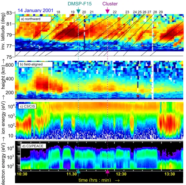
On 14 January 2001, the four Cluster spacecraft approached the magnetopause from the tail lobe, close to the 15:00 MLT meridian. Simultaneous measurements were made using a wide array of ground-based instrumentation. An overview of this pass and of the instrumentation deployed is given by Opgenoorth et al. (2001, this issue), who also study the intersection of the exterior particle cusp by the Cluster craft at about 13:30 UT. In addition, combined Cluster and ground-based observations of polar cap patches, seen be-tween 08:00 and 09:30 on this day, are discussed by Lock-wood et al. (2001, this issue). Figure 1 presents and overview of the data recorded by Cluster and EISCAT Svalbard Radar (ESR) between 10:30 and 14:00. Figure 1a shows the plasma concentrations seen by the ESR beams pointing at low (30◦) elevation along the northward magnetic meridian. Figure 1b shows the plasma concentrations along the other ESR beam, aligned with the local magnetic field direction. Figure 1c shows the ions seen by the CIS instrument of the Cluster C3 spacecraft: differential energy flux is contoured in an energy-time spectrogram format. Figure 1d shows the electrons seen
M. Lockwood et al.: Coordinated Cluster and ground-based instrument observations 1619 ele ctron energ y (e V) → ion energ y (e V) → hei ght ( km) → inv. la titude (deg) time (hrs : min) → 83 81 79 77 75 14 January 2001 104 103 102 a) northward b 600 400 200 d) C3/PEACE 18 19 20 21 22 23 24 25 26 27 28 29 b) field-aligned 10:30 11.30 12:30 13:30 DMSP-F15 Cluster c) C3/CIS 104 -103 -102 10
-Fig. 1. Observation of transient events seen by Cluster and the EISCAT Svalbard Radar (ESR) on 14 January 2001. (a) The plasma
concentrations seen in the ionosphere along the low elevation (30◦) poleward beam of the ESR, are colour-coded as a function of time and latitude. The centre of poleward-moving events are marked with a black line which is numbered in continuation of the events earlier on the same day, as studied by Lockwood et al. (2001, this issue). (b) The observations along the field-aligned ESR beam are shown as a function of time and altitude. (c) An energy-time spectrogram of differential energy flux of ions, integrated over all pitch angles, as observed by the CIS instrument on Cluster C3. (d) An energy-time spectrogram of the count rate of electrons observed by the HEEA detector of the PEACE instrument on Cluster C3 in zone 11 (electrons moving in the +ZGSE direction). The ESR and CIS data are colour-coded using the same
scales as in Fig. 1 of Opgenoorth et al. (2001, this issue). The PEACE data are scaled using the same scale as in Fig. 8 of the present paper. The vertical dashed lines give the times of closest conjunction of the ESR and Cluster (mauve) and the ESR and the DMSP-F15 satellite (green).
in zone 11 of the HEEA detector (i.e. of electrons moving in the +ZGSE direction) of the PEACE instrument, also on
the Cluster spacecraft C3: count-rates are contoured in an energy-time spectrogram format.
In this paper, we concentrate mainly on the data taken be-tween 11:00 and 12:30 which includes close conjunctions of the ESR with the DMSP-F15 satellite and the Cluster space-craft at about 11:44 and 12:20 UT, respectively (marked by the green and purple dashed lines in Fig. 1). In this interval, the Cluster craft were observing the dayside magnetospheric population often termed boundary plasma sheet (BPS, e.g.
Newell and Meng, 1992) with frequent, but brief, excur-sions into the low latitude boundary layer (LLBL). These are marked by the appearance of low-energy sheath ions and electrons (predominantly at energies below 500 eV) and the partial or complete disappearance of magnetospheric elec-trons (predominantly at energies above 500 eV), but not of the magnetospheric ions. Clear-cut examples of these LLBL entries are seen around 11:23, 11:37 and 12:52, with a more complex but long-lived example around 12:10. Other short-lived examples are also seen before the cusp convected east-ward over the craft at around 13:30 (see Opgenoorth et al.,
1620 M. Lockwood et al.: Coordinated Cluster and ground-based instrument observations 2001, this issue) and further examples were seen in the
in-terval after the cusp intersection and before the passage of the satellites through the magnetopause (not shown here, see Opgenoorth et al., 2001, this issue).
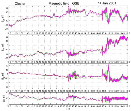
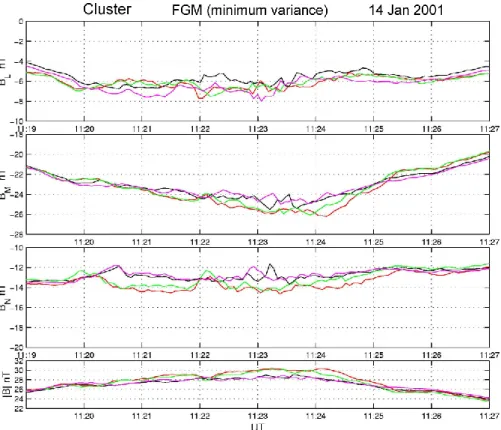
Figure 1a shows that the poleward-pointing ESR beam continued to observe poleward-moving events, as it had dur-ing the prior interval of southward IMF (see Lockwood et al., 2001, this issue). The numbering scheme used in Fig. 1 is a continuation of that used in the previous paper. How-ever, these events were slightly less frequent and migrated poleward at a somewhat lower phase speed that they had ear-lier (see Fig. 8 of Lockwood et al., 2001, this issue). An-other difference is that these were not, in general, seen by the field-aligned ESR beam (Fig. 1b). Blelly et al. (2001, private communication) have shown that even the event that was seen by the ESR field-aligned beam at around 11:00, does not have the same origin as the events (numbers 20, 21, and 22) seen in the northward-pointing beam. At this time the convection pattern was evolving in a complex way, following the northward turning of the IMF. Figure 2 is an overview of the magnetic field seen by the FGM instruments on the four Cluster spacecraft on this pass: the four panels give BX, BY and BZ in GSE coordinates and |B|. All four
spacecraft show almost identical variations on the timescales shown here. At the start of the plot at 11:00 [BX]GSE > 0,
but this reverses to [BX]GSE < 0 after about 12:00
com-bined with the plasma data (which show a progression from lobe to mantle to dayside plasma sheet), we interpret this as a motion of the spacecraft from tail-like field lines onto dayside field lines; [BY]GSE < 0 is true at all times when
Cluster is in the magnetosphere, which is as expected for the 15 MLT location of the spacecraft; [BZ]GSE <0 until about
12:05, it is approximately zero for 12:05–13:15, and sub-sequently, [BZ]GSE > 0 for the remainder of the time that
Cluster is within the magnetosphere. Thus, Cluster was ini-tially observing the interior boundary layers LLBL/BPS (i.e. on southward-pointing field lines in the magnetic cusp fun-nel, half way along the boundary field lines between the exte-rior magnetopause and middle altitudes). From 12:05–13:15, Cluster was observing the field lines that connect the interior and exterior, and interior boundaries (BZ ≈ 0), and
subse-quently, the spacecraft observed the exterior magnetopause boundary layers (BZ>0) where they intersected the exterior
cusp at about 13:30 (Opgenoorth et al., 2001, this issue). For the LLBL entry event around 11:23, which is studied in this paper in detail, the spacecraft are in the interior boundary lay-ers (BZ <0). We also look at an event around 12:10, when
the spacecraft were in the region with BZ ≈0 and an event
around 12:53. Within this last event is a pulse of positive BZ,
and this event takes place when the spacecraft are close to the exterior boundary layers (BZ >0). Figure 3 of Lockwood
et al. (2001, this issue) gives the interplanetary magnetic field seen by the ACE spacecraft on this day. Opgenoorth et al. (2001, this issue) report a very high cross-correlation of the clock angle of the magnetosheath field (in the GSE
ZY plane) seen by Cluster, once it had emerged from the magnetosphere after 15:00 UT, with the same angle seen by
ACE. The conservation of clock angle across the bow shock reveals a lag of 74 min between ACE and the magnetosheath. Lockwood et al. (2001, this issue) have cross-correlated mag-netic perturbation seen by the IMAGE magnetometer chain before the northward turning and derived a lag between ACE and the ionosphere that fluctuated around 75 min. Given that the propagation delay from the magnetopause to the dayside auroral ionosphere is typically 1–2 min, these lag estimates are highly consistent. In the interval studied in this paper, the lagged IMF is predominantly northward: the effects of a clear northward turning of the IMF seen by ACE around 09:50 are clearly detected around 11:00 in magnetometer de-flections, and the transpolar voltage from the potential model fits to the SuperDARN radar data. Here we concentrate on the Cluster data taken in intervals marked B and C in Fig. 3 of Lockwood et al. (2001, this issue). When allowing for the derived propagation lag of 75 min, these intervals correspond to 11:19–11:27 UT and 12:00–12:20 UT, both of which have northward IMF (for interval B, BZ ≈ +3 nT, BY ≈ +1.5 nT
in GSM coordinates, giving a clock angle θIMF ≈ 26◦; for
interval C, BZ ≈ +3 nT, BY ≈ −3 nT, giving θIMF ≈45◦).
However, both follow intervals in which the IMF BZ
compo-nent fell briefly to near to zero (θIMF≈90◦), with a positive
IMF BY.
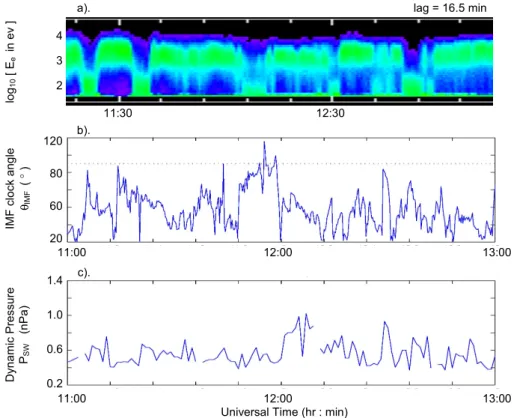
This association is stressed in Fig. 3 which shows the PEACE electron data from Fig. 1d with the IMF clock angle in GSM (θIMF, Fig. 3b), and the solar wind dynamic pressure
data observed by ACE (PSW, Fig. 3c). The interplanetary
data are plotted on a time scale that is lagged by the nomi-nal delay of 75 min, but an additionomi-nal offset of 16.5 min has been introduced between the PEACE data and the ACE data plots, making a total lag of 91.5 min. This lag provides a good alignment of the event seen by Cluster around 12:10, when Cluster and the ESR were in close conjunction. How-ever, Fig. 3 also demonstrates that there is a general corre-spondence between the onset of other LLBL events and the increases in the IMF clock angle. There is no correspondence between the solar wind dynamic pressure changes and this or any other lag. The origin of the additional lag of 16.5 min, however, requires an explanation before the LLBL events can be associated with the swings of the IMF vector toward the magnetospheric equatorial plane (the rises in θIMF).
2.1 DMSP-F15 observations
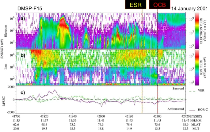
Figure 4 shows (a) the electrons and (b) the ions observed by DMSP-F15 as it passed equatorward, moving close to the ESR field-aligned beam around 11:44. The path of the satellite relative to the two ESR beams is given in Fig. 5 in invariant latitude with Magnetic Local Time (3-MLT) co-ordinates. In Fig. 4, the differential energy flux is plotted as a function of energy (increasing upward) and observation time. The satellite entered the polar cap, passing through an auroral oval showing a series of inverted-V electron arcs at 11:36–11:39 UT, at around 3 = 70◦ and 19:00 MLT. The purple line in Fig. 4c shows the horizontal convection veloc-ity perpendicular to the satellite track, which changed from
M. Lockwood et al.: Coordinated Cluster and ground-based instrument observations 1621
Fig. 2. The magnetic field observed by the four Cluster spacecraft at 11:16 UT on 14 January 2001. The plots shows the BX, BY and BZ
components in the GSE frame and the field magnitude |B|. Data from spacecraft C1, C2, C3 and C4 are coloured (respectively) black, red, green and magenta. (Note: in this figure, data have been plotted in the order of C1, C2, C3 and then C4 and since the data are very similar on this time scale, the magenta line for C4 has covered much of the other three lines).
sunward (i.e. from right to left when looking forward along the orbit) to weakly “anti-sunward” (i.e. from left to right across the orbit) close to the poleward edge of this auroral oval. The segment of the DMSP-F15 path that revealed the sunward flow channel and inverted-V events is marked with a thicker line in Fig. 5. At the poleward edge of the inverted-V events, the satellite observed a convection reversal boundary, with anti-sunward flow persisting thereafter.
The satellite was then briefly within a region where it ob-served polar cap precipitation, with brief intersections of magnetosheath. No significant ion flux was seen and the convection was anti-sunward. This persisted until about 11:41:30, when the satellite began to observe persistent sheath electron fluxes. This segment of the orbit is also marked with a thick line in Fig. 4, labelled sheath-like elec-trons because the spectrum is notably lacking in the lowest energy electrons of the sheath distribution. At this time, weak fluxes of ions are seen at about 3–20 kV. Just before the satel-lite’s closest conjunction with the field-aligned ESR beam (at around 11:44, orange and black dashed line), the elec-tron spectrum becomes a low-flux, low-energy sheath dis-tribution which persists until the satellite passes through the open-closed boundary (OCB), estimated here to be at 11:45 (red and black dashed line). The OCB is identified by the disappearance of the weak sheath electron population and the
onset of persistent BPS electrons. After 11:45, there is a brief dispersed electron event at low-energies and a brief drop out of the BPS electrons (at energies above about 1 keV). This may be a brief re-encounter with the OCB, but this is not as clear-cut as in the example presented by Lockwood et al. (2001, this issue). The OCB location is also marked on Fig. 5.
2.2 Convection and magnetometer observations
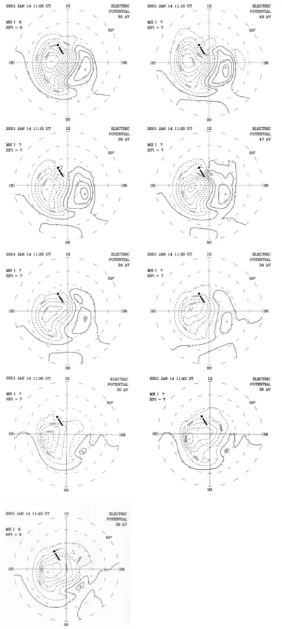
Figure 5 also plots the flow streamlines (equipotentials 5 kV apart) derived by the AMIE technique for 11:40–11:45 UT, when the DMSP-F15 satellite was close to the ESR. The technique has used observations by the SuperDARN radars, ground-based magnetometers, the EISCAT radars and the DMSP satellites. The pattern shows a dominant dusk cell with only a weak dawn cell. The pattern appears to show a convection throat at high-latitudes (3 ≈ 80 − 85◦) in the morning sector with eastward and poleward flow into the po-lar cap, suggesting negative IMF BY (Heelis et al., 1976).
However, the lagged IMF data at this time gives positive IMF BY and such an interpretation would place both the
ESR beams on closed field lines, which is inconsistent with the OCB location deduced from Fig. 4. This will be dis-cussed again below. The evolution of the pattern to the form shown in Fig. 5 is presented in Fig. 6. At 11:05, the lagged
1622 M. Lockwood et al.: Coordinated Cluster and ground-based instrument observations
11:00 12:00 13:00 Universal Time (hr : min)
Dyn a m ic P re ssu re PSW (n P a ) IMF clock an gle θIMF ( ° ) 1.4 1.0 0.6 0.2 120 80 60 20 b). c). lo g10 [ E e in e v ] 4 3 2
a). lag = 16.5 min
11:00 12:00 13:00 11:30 12:30
Fig. 3. (a) The PEACE data shown in Fig. 1d and compared with (b) the IMF clock angle θIMFin GSM coordinates, as observed by ACE and
(c) the solar wind dynamic pressure, PSW, also observed by ACE. The ACE data are plotted against lagged time, using the nominal 75 min.
lag derived independently by Lockwood et al. (2001, this issue) and Opgenoorth et al. (2001, this issue) for, respectively, before and after the period of interest in this paper. An additional lag of 16.5 min has been introduced to obtain a good correspondence between the transient LLBL entries seen by Cluster and the increases in θIMFto near 90◦.
IMF had turned northward, but the convection pattern had yet to respond in any significant way (the transpolar voltage is 55 kV, which was the value it had during the prior period of southward IMF, see Fig. 3, Lockwood et al., this issue), other than a small patch of low flow which appeared just to the west noon. The flow pattern had a vigorous dawn cell as well as the dominant dusk cell and the flows in the day-side polar cap were poleward and weakly westward, which is consistent with the weakly positive IMF BY. At 11:10,
the transpolar voltage had dropped to 49 kV and the slow flow feature evolved into an unusual distortion of the dusk cell around noon. The perturbation to the flow had addi-tional anti-sunward flow just to the west of the ESR, with additional sunward flow to the west of that paint. By 11:15, only the additional poleward flow could be resolved, having migrated towards dusk, such that it was to the east of the ESR. The transpolar voltage had fallen to 39 kV. At 11:20, the transpolar voltage had risen again to 47 kV, primarily due to a second enhancement in poleward flow, which like the previous one, appears first near noon. The first enhancement in poleward flow can still be defined and has moved further east (but at a slower speed), occuring around 16:00 MLT at this time. After 11:25, the transpolar voltage was roughly constant at a baselevel of about 35 kV. This value is likely to reflect the rate of open flux destruction in the tail, in which
case further enhancements in the dayside voltage are not go-ing to be reflected in the transpolar voltage. It appears that poleward flow features form near noon at 11:10, 11:20 and then migrate east.
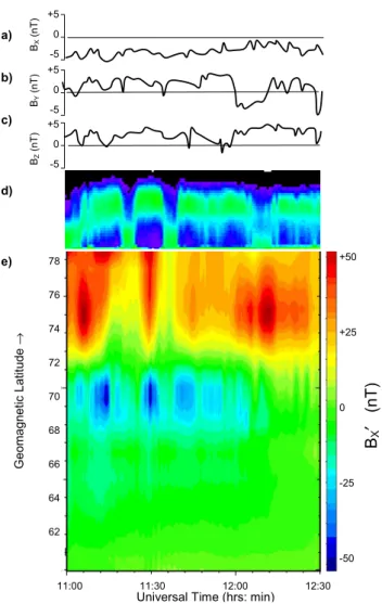
This eastward propagation may offer an explanation of some or all of the delay of 16 min between the IMF clock angle changes and the seemingly associated LLBL entry event. A more detailed study of the enhancements at the ESR/IMAGE meridian is presented in Fig. 7, which shows the 3 components of the lagged IMF data (by the nominal 75 min), the electron data seen by PEACE-C4 (panel d), and the upward continuation of the ground BXperturbation, BX0,
seen by the IMAGE chain, in the same format as used by Lockwood et al. (2001, this issue). A positive X (north-ward) component (BX0 > 0) is a response to an eastward
current. If the magnetometers are responding to a Hall cur-rent in the E-region (i.e. horizontal uniformity of conductiv-ities can be assumed), this corresponds to a westward con-vection velocity in the F-region. Note that the yellow and red colours reveal positive BX0 (eastward current and thus
westward flow) whereas green and blue reveal negative BX0
(westward current and thus eastward flow). Between 11:00 and 12:00 (roughly 14:45–15:45 MLT), westward flow was seen poleward of weaker eastward current south of the ESR; only the former of these can be seen in the AMIE flow
pat-M. Lockwood et al.: Coordinated Cluster and ground-based instrument observations 1623
DMSP-F15 14 January 2001
ESR
OCB
a)
b)
c)
Fig. 4. Energy-time spectrograms for (a) electrons and (b) ions observed by DMSP-F15 as it passed equatorward in close conjunction with
the ESR along the path shown in Fig. 5. In both cases, the differential energy flux is plotted as a function of energy (increasing upward) and observation time, ts. (c) Shows the vertical (green) and horizontal (purple) components of the ion velocity (the horizontal component is
perpendicular to the satellite track such that positive values have a sunward component and negative values have an anti-sunward component. The orange-and-black dashed line gives the time of closest conjunction with the ESR field-aligned beam and the red-and-black line gives the open-closed field line boundary (OCB) defined from the energetic magnetospheric electrons.
terns shown in Fig. 6. Figure 7e shows clear increases in
BX0 a few minutes (respectively about 7 and 5 min) before
the first two LLBL entry events at Cluster (at around 11:23 and 11:37 UT, Fig. 7d). Note that the first of these is clear at the highest latitudes, but is slightly masked by the (declin-ing) residue of enhanced BX0due to the southward IMF prior
to the northward turning. For these two events, the relevant part of the IMAGE magnetometer chain is at an MLT 49 and 35 min ahead of Cluster. For the third LLBL event around 12:10, there is an almost a coincident enhanced BX0 event.
In this third case, IMAGE is at essentially the same MLT as Cluster. These data are consistent with events propagating eastward at about 7 min of MLT per min (roughly 0.9 km s−1 at ionospheric altitudes), and giving both the enhanced flow signatures (detected as BX0 increases) and a transient entry
of the Cluster spacecraft into the LLBL.
If these events are also manifest as the poleward flow en-hancements near noon as seen in Fig. 6 (that commence in the intervals from 11:05–11:10 and 11:15–11:20), they must have moved from noon to the IMAGE meridian at the higher average speed of 14 min of MLT per 1 min (approximately 1.8 km s−1) between 12 MLT and 14 MLT (double the av-erage speed between IMAGE and Cluster at 14 MLT and 15 MLT). This is consistent with the flow perturbations
high-lighted in Fig. 6, as they move rapidly initially east and then they slow down. Thus, the first detected signatures of the events seen by Cluster appear to be the flow enhancements near noon at about 11:07:30 and 11:17:30 in the AMIE con-vection plots. These are both just 5 min after the transient swings of the IMF to a near 90◦ clock angle and if one
al-lows for the magnetopause to ionosphere propagation delay of 1–2 min, this is then within the uncertainty of the nominal lag estimate of 75 min.
2.3 Cluster observations
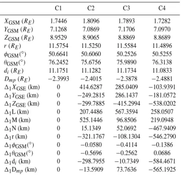
Figures 8 to 11 present a detailed analysis of the Cluster data from the interval of 11:19 to 11:27, which includes the sec-ond of the transient LLBL events shown in Fig. 1. Table 1 gives the coordinates of the Cluster spacecraft for this inter-val: the X, Y and Z coordinates in GSM; the geocentric dis-tance, r; the latitudinal and longitudinal angles, φGSM and θGSM, respectively; the field-aligned distance to the
iono-sphere, di; and the smallest distance of the spacecraft to the
model magnetopause of Shue et al. (1997), Dmp. All of these
parameters are also referenced to spacecraft C1 so, for ex-ample 11XGSM is the difference between the XGSM of the
1624 M. Lockwood et al.: Coordinated Cluster and ground-based instrument observations 35kV 11:40 UT 14 January 2001 MLT = 00 hrs 06 12 18 Λ = 60º 70º Cluster footprint DMSP-F15
ESR field-aligned beam ESR low elevation beam
-5kV 0 kV +10kV +20kV OCB sheath-like electrons inverted-V electrons
Fig. 5. An invariant-latitude (1) – MLT map of the convection
equipotentials from the AMIE technique for magnetometer, Super-DARN, EISCAT/ESR and DMSP data post-integrated over the in-terval 11:40–11:45. The path of the DMSP-F15 satellite is shown, with the two thick segments showing where the satellite observed sunward convection and inverted-V electron precipitation and mag-netosheath electron precipitation. The location of the open-closed boundary (OCB, crossed by DMSP-F15 at 11:45) is also marked as are the locations of the two ESR beams and the mapped footprint of the Cluster spacecraft.
are given in km, whereas the coordinates are given in Earth radii (1 RE = 6370 km). The separations are also given in
normal coordinates (L, M, N ). The boundary-normal orientation was first determined from a model since the spacecraft did not intersect the magnetopause until some considerable time after the events discussed here. How-ever, when it did intersect the magnetopause at around 15:30, the boundary-normal coordinates were found by the mini-mum variance technique to be almost exactly the same as those for this model. We employ the minimum variance results that give unit vectors of (l, m, n) and (i, j , k) in the boundary-normal and GSE frames which are related by
l = (0.32i + 0.59j − 0.74k), m = (0.63i − 0.71j − 0.29k),
and n = (0.70i + 0.37j + 0.61k). These values are suffi-ciently accurate to ensure that Bnis relatively small
through-out the interval.
Table 1 shows that spacecraft C3 is closest to the model magnetopause (both 11Dmp and 11N are maxima for this
spacecraft, equal to, respectively, +73.8 km and +52.1 km), whereas C4 is predicted to be at the deepest point in the mag-netosphere (both 11Dmpand 11N are minima of −565.2 km
and −467.9 km); C1 and C2 are at a similar distance from the model boundary and 11Dmpand 11N yield different
an-swers as to which is closest: 11Dmp is −13.6 km for C2,
Table 1. Cluster spacecraft coordinates and separations at 11:23 on
14 January 2001 C1 C2 C3 C4 XGSM(RE) 1.7446 1.8096 1.7893 1.7282 YGSM(RE) 7.1268 7.0869 7.1706 7.0970 ZGSM(RE) 8.9529 8.9065 8.8869 8.8689 r(RE) 11.5754 11.5250 11.5584 11.4896 φGSM(◦) 50.6641 50.6060 50.2526 50.5255 θGSM(◦) 76.2452 75.6756 75.9890 76.3138 di(RE) 11.1751 11.1282 11.1734 11.0833 Dmp(RE) −2.3993 −2.4015 −2.3878 −2.4881 11XGSE(km) 0 414.6287 285.0409 −103.9391 11YGSE(km) 0 −249.2815 286.1437 −181.0572 11ZGSE(km) 0 −299.7885 −415.2994 −538.0202 11L (km) 0 207.4486 567.3594 258.0507 11M (km) 0 525.1446 96.8506 219.0948 11N (km) 0 15.1349 52.0692 −467.9409 11r (km) 0 −321.1767 −108.1304 −546.2790 11φGSM(◦) 0 −0.0580 −0.4114 −0.1386 11θGSM(◦) 0 −0.5696 −0.2562 0.0686 11di(km) 0 −298.7955 −10.7349 −584.4671 11Dmp(km) 0 −13.5909 73.7636 −565.1925
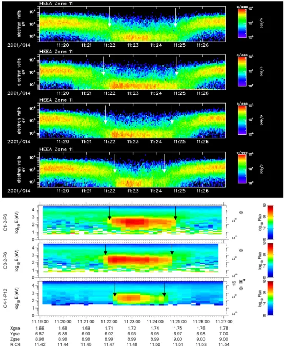
whereas 11N is +15.13 km. Figure 8 compares the
elec-tron and ion data observed by the PEACE and CIS instru-ments on the four spacecraft C4 during this interval. The top four panels show the data, from top to bottom, the HEEA detector of PEACE for spacecraft C1, C2, C3 and C4. Data are shown for zone 11, i.e. the electrons are moving in the
+ZGSE direction. This zone gives a continuous data series
at the highest time resolution. The count rates (proportional to differential energy flux) are shown in spectrogram format as a function of energy and time. Also shown are data from the three functioning CIS ion instruments (on board, in or-der, C1, C3 and C4). The differential energy flux is shown in energy-time spectrogram format, integrated over all pitch angles. The arrows mark the appearance and disappearance of the lowest energy (< 100 eV) magnetosheath electrons in the PEACE data. They are reproduced on the CIS data panels. It can be seen that these points also mark the ap-pearance and disapap-pearance of the largest fluxes of magne-tosheath ions. However, careful inspection reveals that there are some lower fluxes of sheath ions seen outside these two arrows, particularly by C1 and C3. Outside of the arrows, the electron data reveal both a continuously dispersed disap-pearance and reapdisap-pearance of magnetospheric electrons and a similarly dispersed appearance and loss, respectively, of lower energy sheath electrons. This reveals that the space-craft has passed through a layered structure, rather than wit-nessing a transient loss of magnetospheric electrons (for the latter, the highest energy sphere electrons would have reap-peared first and the lowest energy sheath electrons would have disappeared last). This layering is consistent with the satellite passing onto open field lines along which magneto-sphere electrons were lost by flowing out across the
magne-M. Lockwood et al.: Coordinated Cluster and ground-based instrument observations 1625
Fig. 6. The sequence of 5 min integrated AMIE convection patterns for 11:05–11:45. The locations of the two ESR beams are shown in each
1626 M. Lockwood et al.: Coordinated Cluster and ground-based instrument observations G eom a gne tic L ati tude → BX ′ (nT) +50 +25 0 -25 -50 11:00 11:30 12:00 12:30
Universal Time (hrs: min) 78 76 74 72 70 68 66 64 62 60 BZ (nT) BY (nT) BX (n T) +5 0 -5 +5 0 -5 +5 0 -5 a) b) c) d) e)
Fig. 7. (a)–(c) represent the lagged (by 75 min) variations of the
IMF components BX, BY and BZin the GSM reference frame; (d)
the energy-time spectrogram of the electron data seen by PEACE-C4 (as shown in Figs. 1 and 3), and (e) the “upward continuation” of the X component of the magnetic field BX0as a function of latitude and from the IMAGE magnetometer chain. The technique used to derive BX0employs Fourier analysis of the observations of the data from the latitudinal chain of stations on the ground to reconstruct high-resolution latitude variations that would have been observed just below the current layer.
topause, and magnetosheath electrons were gained, by flow-ing in the opposite direction. The time-of-flight dispersion of both reveals that the satellites passed onto field lines that had been open for longer at the event centre before returning to closed field lines. The magnetospheric ions are the apparent difficulty in this interpretation. Figure 8 shows that their flux is not really altered much at all in the event and remains con-stant, even when the magnetosheath ions are present. This cannot be an effect of the longer flight time of the ions (com-pared to electrons of the same energy) since the sheath ions have had time to arrive. Data from the RAPID instrument at higher energies confirms the decrease in flux of magneto-spheric electrons but only small reductions in the flux of the ions (Wilken et al., 2001, this issue). The lack of any
tran-sient decrease and recovery in the magnetosperic ions shows that their maintenance is not due to drifts onto opened then re-closed field lines. Thus, if the satellite is moving onto, and then deeper into open field lines in this event, some pro-cess is maintaining the flux of magnetospheric ions on these newly-opened field lines. The only alternative explanation is that the sheath plasma has been injected onto closed field lines, but this does not explain the loss of the magnetospheric electrons, nor the dispersion ramps outside the arrows.
Figure 9 gives the moments of the ion gas, as observed by the CIS instrument on spacecraft 4. The times of the relevant pair of arrows in Fig. 8 are given by the two vertical lines. The panels show: (a) the proton number density, N(H+); (b) the alpha particle number density, N(He++); (c) the field-parallel ion temperature, T||; (d) the field-perpendicular ion
temperature, T|; and the ion velocity components; (e) VX,
(f) VY; and (g) VZ, in GSE coordinates. The number
den-sity of protons and alpha particles shows the same wave-form, such that the fraction of alpha particles is about 10% throughout. The mixing of the two populations means that the lower temperature sheath plasma depresses the atures in the event, in particular, the perpendicular temper-ature which falls from typical magnetospheric values of the order of 5 × 10⁷K for this location close to the dayside mag-netopause to of the order of 2 × 10⁶K in the event cen-tre which is typical of sheath values for this magnetopause location. The number densities confirm that there is addi-tional plasma outside the event boundaries, particularly in its wake, but they have only a small effect on the average temperatures. At the event centre, the velocities are of the order of [VX]GSE = −20 km s−1, [VY]GSE =25 km s−1and [VZ]GSE = −25 km s−1. Although these point away from
noon around the magnetopause, these are much smaller val-ues than the valval-ues seen once Cluster does emerge from the magnetopause and into the sheath, which average [VX, VY, VZ]GSE= [−170, 65, −70] km s−1(see below). These
char-acteristics clearly define the plasma as being the low-latitude boundary layer (LLBL) with a mixture of magnetospheric plasma and magnetosheath plasma, flowing anti-sunward, but at much slower speed than the sheath itself. (Mozer et al., 1994).
The spacecraft potential is measured by the EFW instru-ment on each spacecraft and varies with the ambient plasma concentration. Figure 10 shows the values for spacecraft C1 (in black), C2 (red), C3 (green) and C4 (blue). All space-craft see the same variation, with minima outside a main central enhancement where the magnetospheric electrons are lost and magnetosheath plasma are gained, respectively. All satellites see a small secondary peak after the main peak, as can be seen in the N[H+] and N[He++] variations in Fig. 9. The signatures are nested to some extent, with C4 entering the event last and emerging from it first. Table 1 shows that C4 is the furthest from the nominal magnetopause location (it has the largest |Dmp|) and thus this supports the concept of a
travelling indentation of the boundary. Nesting is not so clear for the other spacecraft. The order of the observed event du-rations (from longest to shortest) is C2, C3, C1, C4; whereas
M. Lockwood et al.: Coordinated Cluster and ground-based instrument observations 1627
Fig. 8. Observations of the electrons and ions made by the PEACE and CIS instruments of the Cluster spacecraft at 11:19–11:27. (a)–(d) are
energy-time spectrograms of count rates seen by the HEEA detector of PEACE in zone 11 (electrons moving in the +ZGSEdirection) for
spacecraft C1, C2, C3 and C4, respectively. (e)–(g) are energy-time spectrograms of differential number flux observed by CIS for spacecraft C1, C3 and C4. The arrows mark the boundaries of the LLBL event, defined from the lowest energy sheath electrons, and plotted for the same times on the ion spectrograms and in Fig. 10.
the order set by a constant nested signature and the boundary-normal separations 11N (see Table 1) would be C3, C2, C1,
C4. The arrows in Fig. 10 are at the same times as those in Fig. 8: they are colour-coded using the same scheme as the graphs. The duration and nesting of the events defined this way are similar to those derived from the EFW spacecraft potential data.
Cross-correlating the signatures seen by EFW at the space-craft gives a phase lag between spacespace-craft, which can be used to give one estimate of a phase velocity of [VX, VY, VZ]GSE = [−24, 0, 9] km s−1 , which in turn yields
V|| = 1 km s−1 and V ⊥ = 26 km s−1 in relation to
the average magnetic field direction and [VL, VM, VN] =
[−14.3, −17.7, −11.31] km s−1in boundary-normal coordi-nates. The event is moving anti-sunward into the magneto-sphere, rather than around its dusk flank. Thus, the event demonstrates a field-perpendicular convection of flux tubes, primarily moving in the anti-sunward (−X) direction. Us-ing the Tsyganenko T96 model with appropriate inputs, this velocity maps to a speed of ionosphere Vi ≈ 0.8 km s−1,
in a direction poleward and away from noon around the af-ternoon sector. The core of the event at C2 lasts for 210 s,
1628 M. Lockwood et al.: Coordinated Cluster and ground-based instrument observations
Fig. 9. The moments of the ion gas from spacecraft C3 for the
interval shown in Fig. 8. The panels show: (a) the proton number density, N(H+); (b) the alpha particle number density, N(He++);
(c) the field-parallel ion temperature, T||; (d) the field-perpendicular
ion temperature, T⊥; and the ion velocity components (e) VX, (f) VY, and (g) VZ, in GSE coordinates.
which gives a length of structure at the magnetopause and in its direction of motion of L ≈ 26 × 210 = 5460 km (∼ 1 RE), which mapped to ionosphere gives Li ≈140 km.
Note that the average ion velocities within the event (see Fig. 9) are comparable in magnitude, but not precisely the same as the derived event phase motion. The phase mo-tion is much lower than the exterior sheath speeds seen af-ter the magnetopause crossing. Average velocities for 5 min after the satellites emerge from the sheath (i.e. for 15:09– 15:14 UT) are [VX, VY, VZ]GSE = [−170, 65, −70] km s−1,
giving [VL, VM, VN] = [35.7, −133.0, −137.7] km s−1.
The large negative VN probably indicates that the
satel-lites are already deep into the magnetosheath for much of this time. The best alignment of sheath flow with the nominal boundary plane is seen at 15:06:10, when [VX, VY, VZ]GSE = [−80, 100, −15] km s−1, giving [VL, VM, VN] = [44.5, −117.1 − 28.1] km s−1. For either
estimate, the sheath flow velocity is an order of magnitude larger than the event phase velocity. Both the event
mo-Fig. 10. The spacecraft potentials in the interval shown in mo-Fig. 8,
measured by the EFW instruments on spacecraft C1 (black), C2 (red), C3 (green) and C4 (blue). The arrows correspond to those plotted in Fig. 8.
tion and the sheath flow are towards dusk (negative M com-ponent), but the event motion is equatorward (negative L), whereas the sheath flow is poleward (positive L), indicating that the magnetic curvature force, as well as the sheath flow, is playing a role in the field line evolution. The tension force must have a strong component in the −L direction, implying a high-latitude reconnection site. The large differences be-tween both the magnitude and the direction of the event ve-locity and the sheath veve-locity mean that this event is certainly not a boundary indentation caused by a feature propagating around the magnetosphere in the magnetosheath.
Figure 11 shows the magnetic field observations during this event in the normal frame, using the boundary-normal orientation discussed earlier. Fig. 11 shows no co-herent signal in the boundary-normal component, BN, and
certainly no bipolar signature that could be interpreted as an FTE. However, primarily due to an increase in the BM
component, there is a weak peak in the field magnitude, |B|. Thus, the event appears to be an FTE in all but one respect: it has a dimension of about 1 REin its direction of motion; it
is moving anti-sunward into the polar cap and the motion is field-perpendicular; it contains a mixture of magnetosphere and magnetosheath plasma. The only feature lacking is the bipolar signature in the boundary-normal field.
Unfortunately, skies over Svalbard were cloudy at the time of this event and thus, we could not use auroral imagers to ob-serve any corresponding phase motion in the mid-afternoon auroral ionosphere. However, after the skies cleared, such observations were possible for the less clear-cut event around 12:10. These are discussed in the next section. For compari-son, Fig. 12 shows the PEACE and CIS data for this event, in the same format as Fig. 8. Many of the same features are