HAL Id: hal-00180548
https://hal.archives-ouvertes.fr/hal-00180548
Submitted on 9 Nov 2007
HAL is a multi-disciplinary open access
archive for the deposit and dissemination of
sci-entific research documents, whether they are
pub-lished or not. The documents may come from
teaching and research institutions in France or
abroad, or from public or private research centers.
L’archive ouverte pluridisciplinaire HAL, est
destinée au dépôt et à la diffusion de documents
scientifiques de niveau recherche, publiés ou non,
émanant des établissements d’enseignement et de
recherche français ou étrangers, des laboratoires
publics ou privés.
An Abstract Interpretation-based Combinator for
Modelling While Loops in Constraint Programming
Tristan Denmat, Arnaud Gotlieb, Mireille Ducassé
To cite this version:
Tristan Denmat, Arnaud Gotlieb, Mireille Ducassé. An Abstract Interpretation-based Combinator for
Modelling While Loops in Constraint Programming. the 13th International Conference on Principles
and Practice of Constraint Programming (CP’07), Sep 2007, France. pp.00-00. �hal-00180548�
An Abstract Interpretation Based Combinator
for Modelling While Loops in Constraint
Programming
No Author Given
No Institute Given
Abstract. We present the w constraint combinator that models while loops in Constraint Programming. Embedded in a finite domain con-straint solver, it allows programmers to develop non-trivial arithmetical relations using loops, exactly as in an imperative language style. The deduction capabilities of this combinator comes from abstract interpre-tation over the polyhedra abstract domain. This combinator has already demonstrated its utility in constraint-based verification and we argue that it also facilitates the rapid prototyping of arithmetic constraints (power, gcd, sum, ...).
1
Introduction
A strength of Constraint Programming is to allow users to implement their own constraints. CP offers many tools to develop new constraints. Examples include the global constraint programming interface of SICStus Prolog clp(fd) [6], the ILOG concert technology, iterators of the GECODE system [15] or the Con-straint Handling Rules [9]. In many cases, the programmer must provide prop-agators or filtering algorithms for its new constraints, which is often a tedious task. Recently, Beldiceanu et al. have proposed to base the design of filtering algorithms on automaton [5] or graph description [4], which are convenient ways of describing global constraints. It has been pointed out that the natural exten-sion of these works would be to get closer to imperative programming languages [5].
In this paper, we suggest to use the generic w constraint combinator to model arithmetical relations between a finite set of integer variables. This combinator provides a mechanism for prototyping new constraints without having to worry about any filtering algorithm. It is inspired from the while loop of the imperative programmming style. Originally, the w combinator has been introduced in [10] in the context of program testing but it was not deductive enough to be used in a more general context. In this paper, we base the generic filtering algorithm associated to this combinator on case-based reasoning and Abstract Interpre-tation over the polyhedra abstract domain. Thanks to these two mechanisms, w performs non-trivial deductions during constraint propagation. We illustrate that in many cases this combinator can be useful for prototyping new constraints without much effort.
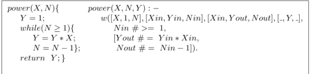
As an example, we illustrate the w combinator on a relation that models y = xn. Note that writing a program that computes the n power of an integer variable x is trivial whereas building finite domain propagators for y = xn is not an easy task for a non-expert user of CP. Figure 1 shows an imperative program (in C syntax) that implements the n power computation of x, along with the corresponding constraint model that exploits the w combinator (in CLP(FD) syntax). In these programs, we suppose that N is positive although this is not a requirement of our approach. It is worth noticing that the w combinator is
power(X, N ){ power(X, N, Y ) :−
Y = 1; w([X, 1, N ], [Xin, Y in, N in], [Xin, Y out, N out], [ , Y, ],
while(N≥ 1){ N in # >= 1,
Y = Y ∗ X; [Y out # = Y in∗ Xin,
N = N− 1}; N out # = N in− 1]).
return Y ;}
Fig. 1. An imperative program for y = xn and a constraint model
implemented as a global constraint. As any other constraint, it will be awoken as soon as X, N or Y have their domain pruned. Moreover, thanks to its filtering algorithm, it can prune the domains of these variables. The following request shows an example where w performs remarkably well on pruning the domains of X, Y and N.
| ?- X in 8..12, Y in 900..1100, N in 0..10, power(X,N,Y).
N = 3, X = 10, Y = 1000
Contributions. In this paper, we detail the pruning capabilities of the w combinator. We describe its filtering algorithm based on case-based reasoning and fixpoint computations over polyhedra. The keypoint of our approach is to re-interpret every constraint in the polyhedra abstract domain by using Linear Relaxation techniques. We provide a general widening algorithm to guarantee termination of the algorithm. The benefit of the w combinator is illustrated on several examples that model non-trivial arithmetical relations.
Organization. Section 2 describes the syntax and semantics of the w opera-tor. Examples using the w operator are presented. Section 3 details the filtering algorithm associated to the combinator. It points out that approximation is crucial to obtain interesting deductions. Section 4 gives some background on abstract interpretation and linear relaxation. Section 5 shows how we integrate abstract interpretation over polyhedra into the filtering algorithm. Section 6 discusses the abstraction. Section 7 concludes.
2
Presentation of the w constraint combinator
This section describes the syntax and the semantics of the w combinator. Some examples enlight how the operator can be used to define simple arithmetical constraints.
2.1 Syntax
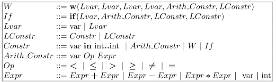
Figure 2 gives the syntax of the finite domain constraint language where the w operator is embedded.
W ::= w(Lvar, Lvar, Lvar, Lvar, Arith Constr, LConstr) If ::= if (Lvar, Arith Constr, LConstr, LConstr)
Lvar ::= var| Lvar
LConstr ::= Constr | LConstr
Constr ::= var in int..int | Arith Constr | W | If Arith Constr ::= var Op Expr
Op ::= < | ≤ | > | ≥ | #= | =
Expr ::= Expr + Expr | Expr − Expr | Expr ∗ Expr | var | int Fig. 2. syntax of the w operator
As shown on the figure, a w operator takes as parameters four lists of vari-ables, an arithmetic constraint and a list of constraints. Let us call these pa-rameters Init, In, Out, End, Cond and Do. The four lists must have the same length. Cond is the constraint corresponding to the loop condition. Do is the list of constraints corresponding to the loop body. In an imperative while loop, body statements compute a new value for the defined variables, depending on the current value of the used variables. A variable can be both used and de-fined. The four lists of variables contain both the used and defined variables of the loop. The Init list contains logical variables representing the initial value of these variables. In variables are the values at iteration n. Out variables are the values at iteration n + 1. End variables are the values when the loop is exited. Note that Init and End variables are logical variables that can be constrained by other constraints. On the contrary, In and Out variables are fresh variables that do not concretely exist in the constraint store. They are local to the w combinator. In variables are involved in the constraints Cond and Do whereas Out variables only appear in the Do constraints. Each variable of Out must be assigned to an expression in the Do constraints.
Line 2 of Figure 2 presents an if combinator. The parameter of type Arith Constr is the condition of the conditional structure. The two parameters of type LConstr are the “then” and “else” parts of the structure. Lvar is the list of variables that appear in the condition or in one of the two branches. We do not further describe this operator to focus on the w operator.
The rest of the language is a simple finite domain constraint programming language with only integer variables and arithmetic constraints.
2.2 Semantics
The solutions of a w constraint is a couple of variable lists (Init, End) such that the corresponding imperative loop with input values Init terminates in a state where final values are equal to End. When the loop embedded in the w combinator never terminates, the combinator has no solution and should fail. This point is discussed in the next section.
2.3 First Example: sum
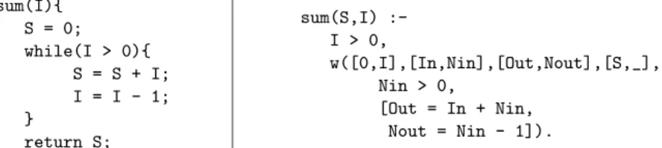
Constraint sum(S,I), presented on Figure 3, constrains S to be equal to the sum of the integers between 1 and I: S = !n
i=1i The factorial constraint
sum(I){ S = 0; while(I > 0){ S = S + I; I = I - 1; } return S; sum(S,I) :-I > 0, w([0,I],[In,Nin],[Out,Nout],[S,_], Nin > 0, [Out = In + Nin, Nout = Nin - 1]). Fig. 3. The sum constraint derived from the imperative code
can be obtained by substituting the line Out = In + Nin by Out = In * Nin. Thanks to the w combinator, sum and factorial are easy to program as far as one is familiar with imperative programming. Note that translating an imperative function into a w operator can be done automatically.
2.4 Second Example: greatest common divisor (gcd)
The second example is more complicated as it uses a conditional statement in the body of the loop. The constraint gcd(X,Y,Z) presented on Figure 4 is derived form the Euclidian algorithm. gcd(X,Y,Z) is true iff Z is the greatest common divisor of X and Y .
3
The filtering algorithm
In this section we present the filtering algorithm associated to the w operator introduced in the previous section. The first idea of this algorithm is derived from the following remark. After n iterations in the loop, either the condition is false and the loop is over, or the condition is true and the statements of the body are executed. Consequently, the filtering algorithm detailed on Figure 5 is basically
gcd(X,Y){ while(X > 0){ if(X < Y){ At = Y; Bt = X; }else{ At = X; Bt = Y; } X = At - Bt; Y = Bt; } return Y; gcd(X,Y,Z) :-w([X,Y],[Xin,Yin],[Xout,Yout],[_,Z], Xin > 0, [if([At,Bt,Xin,Yin], Xin < Yin,
[At = Yin, Bt = Xin], [At = Xin, Bt = Yin]), Xout = At - Bt,
Yout = Bt]).
Fig. 4. The gcd constraint
a constructive disjunction algorithm. The second idea of the algorithm is to use abstract interpretation over polyhedra to over approximate the behaviour of the loop. Function w∞ is in charge of the computation of the over approximation. It will be fully detailed in the next section.
The filtering algorithm takes as input a constraint store ((X, C, B) where X is a set of variables, C a set of constraints and B a set of variable domains), the constraint to be inspected (w(Init, In, Out, End, Cond, Do)) and returns a new constraint store where information has been deduced from the w constraint. ˜X is the set of variables X extended with the lists of variables In and Out. ˜B is the set of variable domains B extended in the same way.
Line 1 posts constraints corresponding to the immediate termination of the loop and launches a propagation step on the new constraint store. As the loop terminates, the variable lists Init, In, Out and End are all equal and the condi-tion is false (¬Cond). If the propagacondi-tion results in a store where one variable has an empty domain (line 2), then the loop must be entered. Thus, the condition of the loop must be true and the body of the loop is executed: constraints Cond and Do are posted (line 3). A new w constraint is posted (line 4), where the initial variables are the variables Out computed at this iteration, In and Out are replaced by new fresh variables (F reshIn and F reshOut) and End variables remain the same. Cond" and Do" are the constraints Cond and Do where vari-able names In and Out have been substituted by F reshIn and F reshOut. The initial w constraint is solved.
Line 5 posts constraints corresponding to the fact that the loop iterates one more time (Cond and Do) and line 6 computes an over approximation of the rest of the iterations via the w∞ function. If the resulting store is inconsistent (line 7), then the loop must terminate immediatly (line 8). Once again, the w constraint is solved.
When none of the two propagation steps has led to empty domains, the stores computed in each case are joined (line 9). The Init and End indices mean that
Input:
A constraint, w(Init, In, Out, End, Cond, Do) A constraint store, (X, C, B)
Output:
An updated constraint store w filtering
1 (Xexit, Cexit, Bexit) := propagate( ˜X, C∧ Init = In = F in ∧ ¬Cond, ˜B)
2 if ∅ ∈ Bexit
3 return ( ˜X, C∧ Init = In ∧ Cond ∧ Do ∧
4 w(Out, F reshIn, F reshOut, End, Cond!, Do!), ˜B) 5 (X1, C1, B1) := propagate( ˜X, C∧ Init = In ∧ Cond ∧ Do, ˜B)
6 (Xenter, Center, Benter) := w∞(Out, F reshIn, F reshOut, End, Cond!, Do!, (X1, C1, B1))
7 if ∅ ∈ Benter
8 return ( ˜X, C∧ Init = In = Out = F in ∧ ¬Cond, ˜B)
9 (X!, C!, B!) := join((Xexit, Cexit, Bexit), (Xenter, Center, Benter))Init,End
10 return (X!, C!∧ w(Init, In, Out, End, Cond, Do), B!)
Fig. 5. The filtering algorithm of w
the join is only done for the variables from these two lists. After the join, the w constraint is suspended and put into the constraint store (line 10).
We illustrate the filtering algorithm on the power example presented on Fig-ure 1 and the following request:
X in 8..12, N in 0..10, Xn in 10..14, power(X,N,Xn). At line 1, posted constraints are:
Xin = X, Nin = N, Yin = 1, Xn = Yin, Nin < 1. This constraint store is in-consistent with the domain of Xn. Thus, we deduce that the loop must be entered at least once. The condition constraint and loop body constraints are posted (we omit the constraints Init = In):
N >= 1, Yout = 1*X, Xout = X, Nout = N-1 and another w combinator is posted:
w([Xout,Yout,Nout],[Xin’,Yin’,Nin’],[Xout’,Yout’,Nout’],[_,Xn,_], Nin’>= 1,[Yout’ = Yin’*Xin’, Xout’ = Xin’, Nout’ = Nin’-1]). Again, line 1 of the algorithm posts the constraints Xn = Yout, Nout < 1. This time, the store is not inconsistent. Line 5 posts the constraints
Nout >= 1, Yout’ = Yout*X, Xout’ = X, Nout’ = Nout - 1, which reduces domains to
Nout in 1..9, Yout’ in 64..144, Xout’ in 8..12. On line 6,
w∞([Xout’,Yout’,Nout’],FreshIn,FreshOut,[_,Xn,_],Cond,Do)is used to infer Xn >= 64. This is a very important deduction as it makes the constraint store inconsistent with Xn in 10..14. So Nout < 1,Xn = X is posted and the fi-nal domains are N in 1..1, X in 10..12, Xn in 10..12. This example points
out that approximating the behaviour of the loop with function w∞ is crucial to deduce information.
On the examples of sections 2.3 and 2.4 some interesting deductions are done. For the sum example, when S is instanciated the value of I is computed. If no value exist, the filtering algorithm fails. Deductions are done even with partial information: sum(S,I), S in 50..60 leads to S = 55, I = 10.
On the request gcd(X,Y,Z), X in 1..10, Y in 10..20, Z in 1..1000, the filtering algorithm reduces the bounds of Z to 1..10. Again, this deduction is done thanks to the w∞ function, which infers the relations Z ≤ X and Z ≤ Y . If we add other constraints, which would be the case in a problem that would use the gcd constraint, we obtain more interesting deductions. For example, if we add the constraint X = 2 ∗ Y , then the filtering algorithm deduces that Z is equal to Y.
Another important point is that approximating loops also allows the filtering algorithm to fail instead of non terminating in some cases. Consider this very simple example that infinitely loops if X is lower than 10.
loop(X,Xn)
:-w([X],[Xin],[Xout],[Xn], X < 10,
[Xout = Xin])
Suppose that we post the following request, X < 0, loop(X,Xn), and apply the case reasoning. As we can always prove that the loop must be unfolded, the algorithm does not terminate. However, the filtering algorithm can be extended to address this problem. The idea is to compute an approximation of the loop after a given number of iterations instead of unfolding more and more the loop. On the loop example, this extension performs well. Indeed the approximation infers Xn < 0, which suffices to show that the condition will never be satisfied and thus the filtering algorithm fails. If the approximation cannot be used to prove non-termination, then the algorithm returns the approximation or con-tinue iterating, depending on what is most valuable for the user: having a sound approximation of the loop or iterating hoping that it will stop.
4
Background
This Section gives some background on abstract interpretation. It first presents the general framework. Then, polyhedra abstract domain is presented. Finally, the notion of linear relaxation is detailed.
4.1 Abstract Interpretation
Abstract Interpretation is a framework introduced in [7] for infering program properties. Intuitively, this technique consists in executing a program with ab-stract values instead of concrete values. The abab-stractions used are such that
the abstract result is a sound approximation of the concrete result. Abstract interpretation is based upon the following theory.
A lattice #L, $, %, &' is complete iff each subset of L has a greatest lower bound and a least upper bound. Every complete lattice has a least element ⊥ and a greatest element ). An ascending chain p1$ p2 $ . . . is a potentially infinite sequence of ordered elements of L. A chain eventually stabilizes iff there is an i such that pj = pi for all j ≥ i. A lattice satisfies the ascending chain condition if every infinite ascending chain eventually stabilizes. A function f : L → L is monotone if p1$ p2 implies f(p1) $ f(p2). A fixed point of f is an element p such that f(p) = p. In a lattice satisfying ascending chain condition, the least fixed point lfp(f) can be computed iteratively: lfp(f) = "i≥0fi(⊥)
The idea of abstract interpretation is to consider program properties at each program point as elements of a lattice. The relations between the program prop-erties at different locations are expressed by functions on the lattice. Finally, computing the program properties consists in finding the least fixed point of a set of equations.
Generally, interesting program properties at a given program point would be expressed as elements of the lattice #P(N), ⊆, ∩, ∪' (if variables have their values in N). However, computing on this lattice is not decidable in the general case and the lattice does not satisfy the ascending chain condition. This problem often appears as soon as program properties to be inferred are not trivial. This means that the fixed points must be approximated. There are two ways for ap-proximating fixed points. A static approach consists in constructing a so-called abstract lattice #M, $M,%M,&M' with a Galois connection #α, γ' from L to M. α : L → M and γ : M → L are respectively an abstraction and concretiza-tion funcconcretiza-tion such that ∀l ∈ L, l $ γ(α(l)) and ∀m ∈ M, m $M α(γ(m)). A Galois connection ensures that fixed points in L can be soundly approximated by computing in M. A dynamic approximation consists in designing a so-called widening operator (noted ∇) to extrapolate the limits of chains that do not stabilize.
4.2 Polyhedra abstract domain
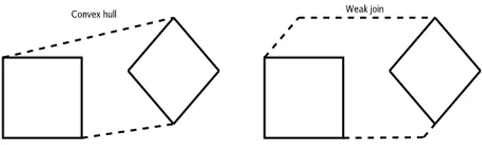
One of the most used instanciation of general abstract interpretation is the inter-pretation over the polyhedra abstract domain [8] or[11]. On this domain, the set of possible values of some variables is abstracted by a set of linear constraints. The solutions of the set of linear constraints define a polyhedron. Each element of the concrete set of values is a point in the polyhedron. In this abstract do-main, the join operator of two polyhedra is the convex hull. Indeed, the smallest polyhedron enclosing two polyhedra is the convex hull of these two polyhedra. However, computing the convex hull of two polyhedra defined by a set of linear constraints requires an exponential time in the general case.
Recent work suggest to use a join operator that over approximates the convex hull [14]. Figure 6 shows two polyhedra with their convex hull and weak join.
Intuitively, the weak join of two polyhedra is computed in three steps. Enlarge the first polyhedron without changing the slope of the lines until it encloses the
Fig. 6. Convex Hull vs Weak Join
second polyhedron. Enlarge the second polyhedron in the same way. Do the intersection of these two new polyhedra.
In many work using abstract interpretation on polyhedra, the standard widen-ing is used. The standard widenwiden-ing operator over polyhedra is computed as fol-lows: if P and Q are two polyhedra such that P $ Q. Then, the widening P ∇Q is obtained by removing from P all constraints that are not entailed in Q. This widening is efficient but not very accurate. More accurate widening operators are given in [2].
4.3 Linear Relaxation of constraints
Using polyhedra abstract interpretation requires to interpret non linear con-straints on the domain of polyhedra. Existing techniques aim at approximating non linear constraints with linear constraints. In our context, the only sources of non linearity are multiplications, strict inequalities and disequalities. These constraints can be linearized as follows:
multiplications Let X and X be the lower and upper bounds of variable X. A multiplication Z = X∗Y can be approximated by the conjunction of inequalities:
(X − X)(Y − Y ) ≥ 0 ∧ (X − X)(Y − Y ) ≥ 0
∧ (X − X)(Y − Y ) ≥ 0 ∧ (X − X)(Y − Y ) ≥ 0 This constraint is linear as the product X ∗ Y can be replaced by Z. In [1], it is proved that this constraint is the smallest linear relaxation of Z = X ∗ Y . Fig.7 shows a slice of the relaxation where Z = 1. The rectangle corresponds to the bounding box of variables X, Y , the dashed curve represents exactly X ∗ Y = 1, while the four solid lines correspond to the four parts of the inequality.
strict inequalities and disequalities Strict inequalities X < V ar (resp. X > V ar) can be rewritten without approximation into X ≤ V ar − 1 (resp. X ≥ V ar + 1), as variables are integers. Disequalities are considered as disjunctions of inequalities. For example, X 4= Y is rewritten into X =< Y −1∨X >= Y +1. Adding the bounds constraints on X and Y and computing the convex hull of the two disjuncts leads to an interesting set of constraints. For example, if X and Y are both in 0..10, the relaxation of X 4= Y is X + Y ≥ 1 ∧ X + Y ≤ 19.
Fig. 7. Relaxation of the multiplication constraint
5
Using abstraction in the filtering algorithm of w
In this section, we detail how abstract interpretation is integrated in the w filtering algorithm. Firstly, we show that solutions of w can be computed with a fixed point computation. Secondly, we explain how abstract interpretation over polyhedra allows us to compute an abstraction of these solutions. Finally, the implementation of the w∞function is presented.
5.1 Solutions of w as the result of a fixed point computation Our problem is to compute the set of solutions of a w constraint: Z ={((x1, . . . , xn), (xf1, . . . , xfn)) | w((x1, . . . , xn), In, Out, (xf
1, . . . , xfn), Cond, Do)} Let us call Sithe possible values of the loop variables after i iterations in a loop. When i = 0 possible variables values are the values that satisfy the domain constraint of Init variables. We call Sinit this set of values. Thus S0= Sinit. Let us call T the following set:
T ={((x1, . . . , xn), (x"
1, . . . , x"n)) | (x1, . . . , xn) ∈ Sinit∧ ∃i(x"1, . . . , x"n) ∈ Si} T is a set of couples of lists of values (l, m) such that initializing variables of the loops with values l and iterating the loop a finite number of times produce the values m. The following relation holds
Z ={(Init, End) | (Init, End) ∈ T ∧ End ∈ sol(¬Cond)}
where sol(C) denotes the set of solutions of a constraint C. The previous formula expresses that the solutions of the w constraint are the couples of lists of values (l, m) such that initializing variables of the loops with values l and iterating the loop a finite number of times leads to some values m that violate the loop condition.
In fact, T is the least fixed point of the following equation: Tk+1= Tk
∪ {(Init, Y ) | (Init, X) ∈ Tk
∧ (X, Y ) ∈ sol(Cond ∧ Do})} (1) T0= {(Init, Init) | Init ∈ Sinit} (2)
Cond and Do are supposed to involve only In and Out variables. Thus, composing Tkand sol(Cond∧Do) is possible as they both are relations between two lists of variables of length n.
Following the principles of abstract interpretation this fixed point can be computed by iterating Equation 1 starting from the set T0 of Equation 2.
For the simple constraint: w([X],[In],[Out],[Y],In < 2,[Out = In+1]) and with the initial domain X in 0..3, the fixed point computation proceeds as follows. T0= {(0, 0), (1, 1), (2, 2), (3, 3)} T1= {(0, 1), (1, 2)} ∪ T0 = {(0, 0), (0, 1), (1, 1), (1, 2), (2, 2), (3, 3)} T2= {(0, 1), (0, 2), (1, 2)} ∪ T1 = {(0, 0), (0, 1), (0, 2), (1, 1), (1, 2), (2, 2), (3, 3)} T3= T2
Consequently, the solutions of the w constraint are given by Z ={(X, Y ) | (X, Y ) ∈ T3
∧ Y ∈ sol(In ≥ 2)} = {(0, 2), (1, 2), (2, 2), (3, 3)}
Although easy to do on the example, iterating the fixed point equation is undecidable because Do can contain others w constraints. Thus, Z is not com-putable in the general case.
5.2 Abstracting the fixed point equations
We compute an approximation of T using the polyhedra abstract domain. Let P be a polyhedron that over approximates T , which means that all elements of T are points of the polyhedron P . Each list of values in the couples defining T has a length n thus P involves 2n variables. We represent P by the conjunction of linear equations that define the polyhedron.
The fixed point equations become:
Pk+1(Init, Out) = Pk& (Pk(Init, In) ∧ Relax(Cond ∧ Do))Init,Out (3) P0(Init, Out) = α(Sinit) ∧ Init = Out (4) Compared to equations 1 and 2, the computation of the set of solutions of constraint C is replaced by the computation of a relaxation of the constraint C. Relax is a function that computes linear relaxations of a set of constraints using the relaxations presented in Section 4.3. PL1,L2 denotes the projection
of the linear constraints P over the set of variables in L1 and L2. Projecting linear constraints on a set of variables S consists in eliminating all variables not belonging to S. Lists equality L = M is a shortcut for ∀i ∈ [1, n]L[i] = M[i],
where n is the length of the lists and L[i] is the ith element of L. P1& P2denotes the weak join of polyhedron P1 and P2presented in Section 4.2.
In Equation 4, Sinit is abstracted with the α function. This function com-putes a relaxation of the whole constraint store and projects the result on Init variables.
An approximation of the set of solutions of a constraint w is given by Q(Init, In) = P (Init, In)∧ Relax(¬Cond) (5) We detail the abstract fixed point computation on the same example as in the previous section. As the constraints Cond and Do are almost linear their relaxation is trivial: Relax(Cond ∧ Do) = Xin≤ 1, Xout= Xin+ 1. Xinis only constrained by its domain, thus α(Sinit) = Xin≥ 0 ∧ Xin≤ 3. The fixed point is computed as follows
P0(Xin, Xout) = Xin≥ 0 ∧ Xin≤ 3 ∧ Xin= Xout
P1(Xin, Xout) = (P0(Xin, X0) ∧ X0≤ 1 ∧ Xout = X0+ 1)Xin,Xout
& P0(Xin, Xout)
= (Xin≥ 0 ∧ Xin≤ 1 ∧ Xout= Xin+ 1) & P0(Xin, Xout) = Xin≥ 0 ∧ Xin≤ 3 ∧ Xout≤ Xin+ 1 ∧ Xout ≥ Xin P2(Xin, Xout) = (P1(Xin, X1) ∧ X1≤ 1 ∧ Xout = X1+ 1)Xin,Xout
& P1(Xin, Xout)
= (Xin≥ 0 ∧ Xin≤ 3 ∧ Xin≤ Xout− 1) & P1(Xin, Xout) = Xin≥ 0 ∧ Xin≤ 3 ∧ Xout≤ Xin+ 2 ∧ Xout ≥ Xin∧ Xout ≤ 4 P3(Xin, Xout) = (P2(Xin, X2) ∧ X2≤ 1 ∧ Xout = X2+ 1)Xin,Xout
& P2(Xin, Xout)
= (Xin≥ 0 ∧ Xin≤ 3 ∧ Xin≤ Xout− 1) & P2(Xin, Xout) = P2(Xin, Xout)
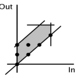
Figure 8 shows the difference between the exact fixed point computed with the exact equations and the approximate fixed point. The points correspond to elements of T3 whereas the grey zone is the polyhedron defined by P3.
An approximation of the solutions of the w constraint is Q = P3(Xinit, Xend) ∧ Xend≥ 2
= Xend≥ 2 ∧ Xend≤ 4 ∧ Xin≤ Xend∧ Xin≤ 3 ∧ Xin≥ Xend− 2 On the previous example, the fixed point computation converges but it is not always the case. Widening can address this problem. The fixed point equation becomes:
Pk+1(Init, Out) = Pk(Init, Out)∇ (Pk
& (Pk(Init, In) ∧ Relax(Cond, Do))Init,Out) In this equation ∇ is the standard widening operator presented in Section 4.2.
Fig. 8. Exact vs approximated fixed point
5.3 w∞: implementing the approximation
In Section 3, we have presented the filtering algorithm of the w operator. Here, we detail more concretely the integration of the abstract interpretation over polyhedra into the constraint combinator w via the w∞ function.
w∞ is an operator that performs the fixed point computation and commu-nicates the result to the constraint store. Figure 9 describes the algorithm. All the operations on linear constraints are done with the clpq library [12].
Input:
Init, In, Out, End vectors of variables
Cond and Do the constraints defining the loop A constraint store (X, C, B)
Output:
An updated constraint store w∞ :
1 Pi+1:= project(relax(C, B), [Init])∧ Init = Out 2 repeat
3 Pi:= Pi+1
4 Pj:= project(Pi
∧ relax(Cond ∧ Do, B), [Init, Out]) 5 Pk:= weak join(Pi, Pj)
6 Pi+1:= widening(Pi, Pk)
7 until includes(Pi, Pi+1) 8 Y := Pi+1
∧ relax(¬Cond, B) 9 (C!, B!) := concretize(Y )
10 return (X, C!∧ w(Init, In, Out, End, Cond, Do), B!)
Fig. 9. The algorithm of w∞operator
This algorithm summerizes all the notions previously described. Line 1 com-putes the initial value of P . It implements the α function introduced in Equa-tion 4. The relax funcEqua-tion computes the linear relaxaEqua-tion of a constraint C given
the current variables domains, B. When C contains another w combinator, the corresponding w∞ function is called to compute an approximation of the sec-ond w. The project(C, L) function is a call to the Fourier variable elimination algorithm. It eliminates all the variables of C but variables from the list of lists L. Lines 2 to 7 do the fixed point computation following Equation 3. Line 6 performs the standard widening after a given number of iterations in the repeat loop. This number is a parameter of the algorithm. At Line 7, the inclusion of Pi+1 in Pi is tested. includes(Pi, Pi+1) is true iff each constraint of Pi is entailed by the constraints Pi+1.
At line 8, the approximation of the solution of w is computed following Equa-tion 5. Line 9 concretizes the result in two ways. Firstly, the linear constraints are turned into finite domain constraints. Secondly, domains of End variables are reduced by computing the minimum and maximum values of each variable in the linear constraints Y . These bounds are obtained with the simplex algorithm.
6
Discussion
The polyhedra abstract domain is generally used differently from what we pre-sented (see for example [8] or [11]). Usually, a polyhedron denotes the set of linear relations that holds between variables at a given program point. As we want to approximate the solutions of a w constraint, our polyhedra describe relations be-tween input and output values of variables and thus, they involve twice as many variables. In abstract interpretation, the analysis is done only once whereas we do it each time a w operator is awoken. This means that we perform in-context analysis. Indeed, the fixed point equations that we solve depend on the constraint store. This also means that we have to use an efficient analysis. Consequently, we cannot afford to use classical libraries to handle polyhedra, such as [3], because they use the dual representation, which is a source of exponential time computa-tions. Our representation implies, nevertheless, doing many variables elimination with the Fourier elimination algorithm. This remains costly when the number of variables grows. However, the abstraction that we have used to compute an approximation of the solutions of w constraints is only one among others. For example, abstraction on intervals is very efficient but leads to less accurate de-ductions. The octagon abstract domain [13] could be an interesting alternative to polyhedra as it is considered to be a good trade-off between accuracy and efficiency.
7
Conclusion
We have presented a constraint combinator, w, that allows users to make a constraint from an imperative loop. We have shown examples where this com-binator is used to implement non trivial arithmetic constraints. The filtering algorithm associated to this combinator is based on case reasoning and fixed point computation. Abstract interpretation on polyhedra provides a method for
approximating the result of this fixed point computation. The results of the ap-proximation are crucial for pruning variable domains. On many examples, the deductions made by the filtering algorithm are considerable, especially as this algorithm comes for free in terms of development time.
References
1. F. A. Al-Khayyal and J. E. Falk. Jointly constrained biconvex programming. Mathematics of Operations Research, 8(2):273–286, 1983.
2. R. Bagnara, P. M. Hill, E. Ricci, and E. Zaffanella. Precise widening operators for convex polyhedra. In Radhia Cousot, editor, Proc. of the Static Analysis Symp., volume 2694 of Lecture Notes in Computer Science, pages 337–354. Springer, 2003. 3. R. Bagnara, E. Ricci, E. Zaffanella, and P. M. Hill. Possibly not closed convex poly-hedra and the parma polypoly-hedra library. In M. V. Hermenegildo and G. Puebla, editors, Proc. of the Static Analysis Symp., volume 2477 of Lecture Notes in Com-puter Science, pages 213–229. Springer, 2002.
4. N. Beldiceanu, M. Carlsson, S. Demassey, and T. Petit. Graph properties based filtering. In Proccedings of the International Conf. on Principles and Practice of Constraint Programming, pages 59–74, 2006.
5. N. Beldiceanu, M. Carlsson, and T. Petit. Deriving filtering algorithms from con-straint checkers. In Proccedings of the International Conf. on Principles and Prac-tice of Constraint Programming, pages 107–122, 2004.
6. M. Carlsson, G. Ottosson, and B. Carlson. An open-ended finite domain constraint solver. In PLILP, pages 191–206, 1997.
7. P. Cousot and R. Cousot. Abstract interpretation : A unified lattice model for static analysis of programs by construction or approximation of fixpoints. In Proc. of Symp. on Principles of Programming Languages, pages 238–252. ACM, 1977. 8. P. Cousot and N. Halbwachs. Automatic discovery of linear restraints among
variables of a program. In Proc. of Symp. on Principles of Programming Languages, pages 84–96. ACM, 1978.
9. T. Fruhwirth. Theory and practice of constraint handling rules. Special Issue on Constraint Logic Programming, Journal of Logic Programming, 37(1-3), 1998. 10. A. Gotlieb, B. Botella, and M. Rueher. A CLP framework for computing structural
test data. In First International Conf. on Computational Logic, pages 399–413. Springer, 2000.
11. N. Halbwachs, Y-E. Proy, and P. Roumanoff. Verification of real-time systems using linear relation analysis. Formal Methods in System Design, 11:157–185, 1997. 12. C. Holzbaur. OFAI clp(q,r) Manual. Austrian Research Institutefor Artificial
Intelligence, Vienna, 1.3.3 edition.
13. A. Min´e. The octagon abstract domain. Higher-Order and Symbolic Computation, 19:31–100, 2006.
14. S. Sankaranarayanan, M. A. Col`on, H. Sipma, and Z. Manna. Efficient strongly relational polyhedral analysis. In K. S. Namjoshi E. A. Emerson, editor, Proc. of the Verification, Model Checking, and Abstract Interpretation Conf., pages 115– 125. Springer, 2006.
15. C. Schulte and G. Tack. Views and iterators for generic constraint implementa-tions. In Recent Advances in Constraints (2005), volume 3978 of Lecture Notes in Artificial Intelligence, pages 118–132. Springer-Verlag, 2006.