Methods for sensitivity analysis and backward propagation of uncertainty applied on mathematical models in engineering applications

(1)

HAL Id: tel-01945221

https://tel.archives-ouvertes.fr/tel-01945221

Submitted on 5 Dec 2018

HAL is a multi-disciplinary open access archive for the deposit and dissemination of sci-entific research documents, whether they are pub-lished or not. The documents may come from teaching and research institutions in France or abroad, or from public or private research centers.

L’archive ouverte pluridisciplinaire HAL, est destinée au dépôt et à la diffusion de documents scientifiques de niveau recherche, publiés ou non, émanant des établissements d’enseignement et de recherche français ou étrangers, des laboratoires publics ou privés.

models in engineering applications

Iman Alhossen

To cite this version:

Iman Alhossen. Methods for sensitivity analysis and backward propagation of uncertainty applied on mathematical models in engineering applications. Mechanical engineering [physics.class-ph]. Univer-sité Paul Sabatier - Toulouse III, 2017. English. �NNT : 2017TOU30314�. �tel-01945221�

(2)

THÈSE

En vue de l’obtention du

DOCTORAT DE L’UNIVERSITÉ DE TOULOUSE

Délivré par:

Université Toulouse 3 Paul Sabatier (UT3 Paul Sabatier)

Présentée et soutenue par :

Iman ALHOSSEN

le 11 Décembre 2017

Titre :

Méthode d’analyse de sensibilité et propagation inverse d’incertitude

appliquées sur les modèles mathématiques dans les applications d’ingénierie

École doctorale et discipline ou spécialité :

ED MEGEP : Génie mécanique

Unité de recherche :

Institut Clément Ader, CNRS UMR 5312

Directeur(s) de Thèse :

Stéphane Segonds

MCF (HDR), Université Paul Sabatier

Directeur

Florian Bugarin

MCF, Université Paul Sabatier

Co-Directeur

Jury :

Bertrand Wattrisse

PR, Université de Montpellier

Rapporteur

Mhamad Khalil

PR, Université Libanaise

Rapporteur

Adrien Bartoli

PR, Université Clermont Auvergne

Président

Cyril Bordreuil

PR, Université de Montpellier

Examinateur

Fulbert Baudouin

MCF, Université Paul Sabatier

Examinateur

(3)

(4)

Acknowledgment

By the end of this thesis I turned the page to open a new chapter in my academic life. Nearly three years have passed since I came to Toulouse, three years with some dark days, but many light days. So thank GOD for everything, thank GOD for giving me this opportunity to be a PhD student and then thank God for granting me the capability to proceed successfully. Also thanks to all those who have helped me finish this work.

First and foremost thanks to my thesis advisors Stephane Segonds and Florian Bugarin for their endless help during the past three years. I could never have imaged to have ad-visors better than you. I will forever be thankful to you !

Thanks to Christina Villeneuve-Faure for her help and courage especially in the ap-plication of the force spectroscopy.

Thanks to Fulbert Baudoin for his assistance in different parts of this work.

Thanks to Adrien Bartoli for his time and help while developing the models of the application in the domain of computer vision.

Thanks to the reviewers of my thesis Mr. Bertrand Wattrisse and Mr. Mohammad

Khalil for accepting evaluating and revising my work. Thanks to all the members of my

thesis committee for participating in this evaluation.

Thanks to my spiritual supporters Samir and Raafat who taught me how we should be patient in order to reach our goals.

Thanks to my colleagues: Batoul, Donghai, Daniel, Hannah, Jim, Montassar, Menouar, Pierre, Shiqi, Yanfeng, Yiewe, and all the nice people I met in Institute Clement Ader. Thanks to my Lebanese friends for being my second family: Abbas, Alaa, Bilal, Fatima, Muhammad, Mariam, Zainab, and all the members of the group "Muntada Essudfa". Finally thanks to my family for the love, encouragement, and support they have always given to me.

(5)

(6)

Abstract

Approaches for studying uncertainty are of great necessity in all disciplines. While the forward propagation of uncertainty has been investigated extensively, the backward prop-agation is still under studied. In this thesis, a new method for backward propprop-agation of uncertainty is presented. The aim of this method is to determine the input uncertainty starting from the given data of the uncertain output.

In parallel, sensitivity analysis methods are also of great necessity in revealing the influ-ence of the inputs on the output in any modeling process. This helps in revealing the most significant inputs to be carried in an uncertainty study. In this work, the Sobol sensitivity analysis method, which is one of the most efficient global sensitivity analysis methods, is considered and its application framework is developed. This method relies on the computation of sensitivity indexes, called Sobol indexes. These indexes give the effect of the inputs on the output. Usually inputs in Sobol method are considered to vary as continuous random variables in order to compute the corresponding indexes. In this work, the Sobol method is demonstrated to give reliable results even when applied in the discrete case. In addition, another advancement for the application of the Sobol method is done by studying the variation of these indexes with respect to some factors of the model or some experimental conditions. The consequences and conclusions derived from the study of this variation help in determining different characteristics and information about the inputs. Moreover, these inferences allow the indication of the best experimental conditions at which estimation of the inputs can be done.

Keywords: Uncertainty quantification, Backward uncertainty propagation, sensitivity

(7)

(8)

Résumé

Dans de nombreuses disciplines, les approches permettant d’étudier et de quantifier l’influence de données incertaines sont devenues une nécessité. Bien que la propagation directe d’incertitudes ait été largement étudiée, la propagation inverse d’incertitudes demeure un vaste sujet d’étude, sans méthode standardisée. Dans cette thèse, une nouvelle méthode de propagation inverse d’incertitude est présentée. Le but de cette méthode est de déter-miner l’incertitude d’entrée à partir de données de sortie considérées comme incertaines. Parallèlement, les méthodes d’analyse de sensibilité sont également très utilisées pour déterminer l’influence des entrées sur la sortie lors d’un processus de modélisation. Ces approches permettent d’isoler les entrées les plus significatives, c’est a dire les plus in-fluentes, qu’il est nécessaires de tester lors d’une analyse d’incertitudes. Dans ce travail, nous approfondierons tout d’abord la méthode d’analyse de sensibilité de Sobol, qui est l’une des méthodes d’analyse de sensibilité globale les plus efficaces. Cette méthode repose sur le calcul d’indices de sensibilité, appelés indices de Sobol, qui représentent l’effet des données d’entrées (vues comme des variables aléatoires continues) sur la sortie. Nous dé-montrerons ensuite que la méthode de Sobol donne des résultats fiables même lorsqu’elle est appliquée dans le cas discret. Puis, nous étendrons le cadre d’application de la méthode de Sobol afin de répondre à la problèmatique de propagation inverse d’incertitudes. Enfin, nous proposerons une nouvelle approche de la méthode de Sobol qui permet d’étudier la variation des indices de sensibilité par rapport à certains facteurs du modèle ou à certaines conditions expérimentales. Nous montrerons que les résultats obtenus lors de ces études permettent d’illustrer les différentes caractéristiques des données d’entrée. Pour conclure, nous exposerons comment ces résultats permettent d’indiquer les meilleures conditions expérimentales pour lesquelles l’estimation des paramètres peut être efficacement réalisée.

(9)

(10)

List of Figures

1.1 The data fitted to a logarithmic function and to a 4th root function.. . . . 9

1.2 The measurements of the height x1 and the radius of the cylinder x2. . . . 12

1.3 Probabilistic presentation of input uncertainty: (a) continuous distribu-tion, (b) discrete distribution . . . . 13

1.4 Probabilistic propagation of input uncertainty. . . 16

1.5 Scatter plot of sampling techniques: (a) Random sampling, (b) Latin Hy-per cube sampling. . . 17

1.6 Fuzzy membership functions: (a) Triangular, (b) Trapezoidal. . . . 25

1.7 Bayesian inference for backward uncertainty propagation: prior distribu-tion and output data are used to derive a posterior distribudistribu-tion. . . 31

1.8 Output variance decomposition for model of two variables representing the concept of the Sobol’s method for the derivation of the sensitivity indexes. 42

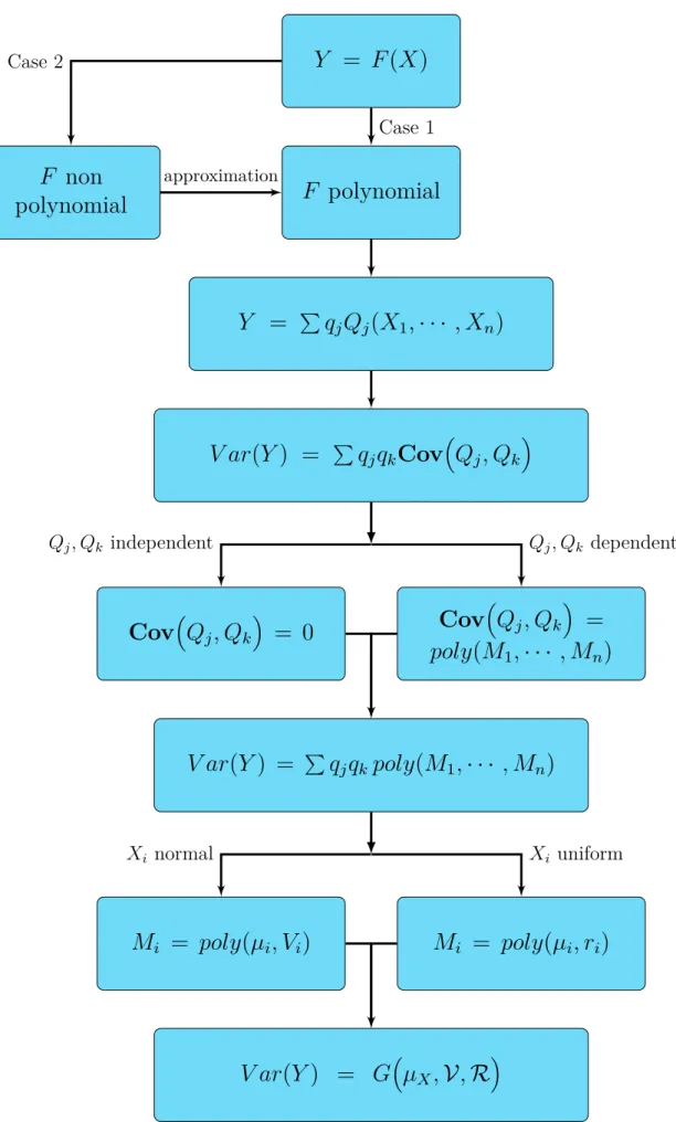
2.1 Flowchart that summarizes Step 1. . . 55

2.2 Uncertain real weight (WR) in terms of the measured weight (Wm). . . 56

2.3 The obtained values of V and r as a function of the number of sample points used. . . 60

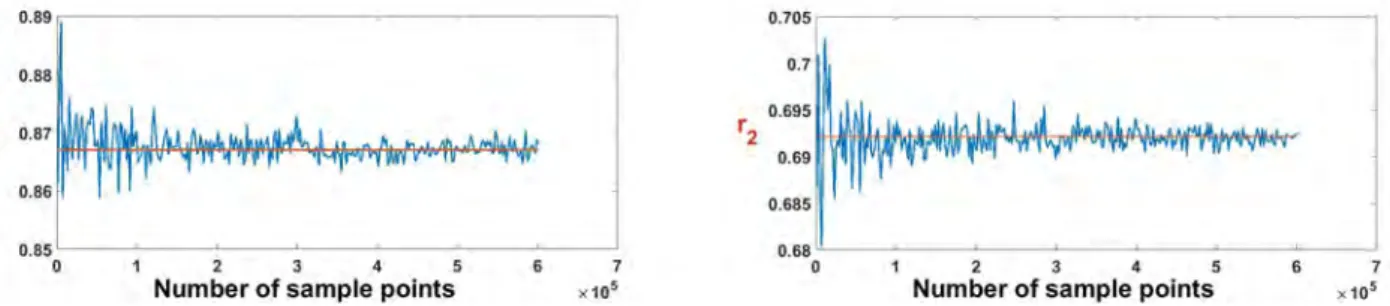
2.4 The obtained values of r1 and r2 as a function of the number of sample points used. . . 61

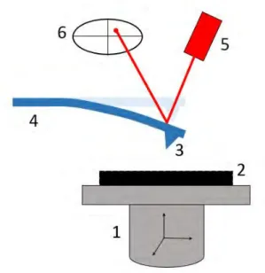
3.1 Schematic of the AFM parts: 1.Piezoscanner 2.Sample 3.Tip 4.Cantilever

5. Laser emitter 6.Photo-detector. . . . 66

3.2 The tip-sample positioning during the different phases of AFM. . . 67

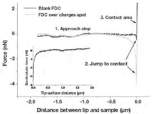
3.3 A typical AFM Force Distance Curve showing the approach stage, the contact stage, and the retract stage. The labels (a), (b), (c), (d), and (e) refer to the phases of the tip-sample positioning of Fig. 3.2. . . 67

3.4 The FDCs while scanning an oxy-nitride dielectric (before and after the effect of the electrostatic force). Their difference produces the EFDC. This figure is extracted from [Villeneuve-Faure et al., 2014]. . . 69

3.5 Sample scheme (electrode is represented in black). . . 70

3.6 Evolution of EFDC as function of electrodes parameters: (a) Width w (bias v and depth d are fixed at 15v and 100nm respectively) and (b) Depth d (bias v and width w are fixed at 15v and 20µm respectively). . . . 72

3.7 The illustration of the logistic curve f(z).. . . 73

3.8 Residuals of the polynomial and logistic regressions. . . 74

3.9 The model Fitted-4PL . . . 74

(13)

3.11 The second order Sobol indexes of d, v, and w. The indexes Sdw, Sdv, and

Svw represent the influence of the interactions between d and w, d and v,

and v and w, respectively, on A, B, C, and D. . . . 79

3.12 The main effect plots of depth d, width w and applied voltage v for each of the 4PL parameters: (a) A, (b) B, (c) C and (d) D. . . . 82

3.13 The Interaction Effects Matrix plot of the parameter A. . . . 84

3.14 one-way interaction plots for the parameters: (a) B, (b) C, and (d) D, in the order : d-w plots, d-v plots and v-w plots. . . . 85

3.15 The difference between the EFDCs obtained experimentally (blue) and the EFDCs obtained using the first order matrix approximation models of A, B, C, and D (red). Different values of (d, v, w) are considered: (a) (10 nm, 6 v, 6 µm) , (b) (100 nm, 8 v, 40 µm), (c) (50 nm, 6 v, 6 µm), and (d) (10 nm, 15 v, 40 µm). . . . 88

3.16 The difference between the EFDCs obtained experimentally (blue) and the EFDCs obtained using the second order matrix approximation models of A, B, C, and D (red). Different values of (d, v, w) are considered: (a) (10 nm, 6 v, 6 µm), (b) (100 nm, 8 v, 40 µm), (c) (50 nm, 6 v, 6 µm), and (d) (10 nm, 15 v, 40 µm). . . . 90

4.1 The pinhole camera. . . 95

4.2 Real vs virtual image by a pinhole camera. . . 96

4.3 Geometric model of the 2D image formation by a pinhole camera. . . 96

4.4 The pixel coordinate system P = {Op; Up, Vp} vs the image plane frame J = {O; U, V}. . . . 97

4.5 A paper template deformed into a cylinder. . . 100

4.6 The 3D reconstruction model in SfT. . . 101

4.7 A scheme of the algorithm SfT_BGCC12I.. . . 108

4.8 The normal at the point M determined by the angle θ. . . . 109

4.9 A scheme of the model ZfT_SfT. . . . 111

4.10 A schematic of the model ZfT_SfT’. . . . 114

4.11 The variation of the first order Sobol indexes SZ and Sf and SN as a function of the depth : (a) For Er with θ ∈ [15◦, 30◦] , (b) For Er with θ ∈ [30◦, 45◦], (c) For Er with θ ∈ [45◦, 60◦], (d) For EN with θ ∈ [15◦_, ₃₀◦_{], (e) For E} N with θ ∈ [30◦, 45◦], (f) For EN with θ ∈[45◦, 60◦] . . . 116

4.12 The variation of the total order Sobol indexes T SZ and T Sf and T SN as a function of the depth : (a) For Er with θ ∈ [15◦, 30◦] , (b) For Er with θ ∈ [30◦, 45◦], (c) For Er with θ ∈ [45◦, 60◦], (d) For EN with θ ∈ [15◦_, ₃₀◦_{], (e) For E} N with θ ∈ [30◦, 45◦], (f) For EN with θ ∈[45◦, 60◦] . . . 120

4.13 The charge transport model. . . 121

4.14 Evolution of the first order Sobol indexes of the injection height barrier w. 124 4.15 Evolution of the first order Sobol indexes of the mobility µ. . . . 125

4.16 Evolution of the first order Sobol indexes of the de-trapping barrier height wtr. . . 127

4.17 Evolution of the first order Sobol indexes of the trapping coefficient B. . . 128

(14)

List of Algorithms

1 First order Sobol indexes of Z, f, and θ as a function of Z with [15◦_, ₃₀◦_{] as} a sampling space for θ . . . 115

2 Total order Sobol indexes of Z, f, and θ as a function of Z with [15◦_, ₃₀◦_] as a sampling space for θ . . . 119

(15)

Nowadays, no one can doubt the basic role of modeling in any scientific process. In short, a model is a systematic description of the relationship between input and output. It aims to imitate, translate, or predict the behavior of real systems. However, undesirable disturbances may prevent a model from achieving its aim perfectly. Indeed, scientists can not be completely accurate during the modeling process, while constructing the model and collecting the input data. This leads to the presence of uncertainty, indicating a state of being unsure about the correctness of the performance of the model. Consequently, it is becoming no longer acceptable to submit any scientific project without providing a comprehensive assessment of the reliability and validity of the results under the effect of uncertainty. For that, studying uncertainty is becoming of a great interest in almost all disciplines, considering it an essential procedure for robust modeling. This manuscript presents our work in developing new methods to deal with uncertainty, and applying such methods in different domains.

The input of a model usually consists of variables and parameters. The variables are said to be uncertain if it is not sure that the values given to run the model are the actual true ones. Mainly, variable uncertainty appears due to imperfect measurements, inherent variability, and incomplete data collection. In addition, the model is said to have pa-rameter uncertainty if its papa-rameters are not surely characterizing the real system. Such uncertainty arises due to poor calibrations, imprecise estimations, or bad curve fittings. Moreover, the model is said to have structural uncertainty if we cannot be confident that the form of the model is accurately imitating the real studied system. Usually, structural uncertainty appears due to ambiguity in the definitions of the given concepts, limitations of the acquired knowledge in the studied domain, or difficulties in some systems to be represented as equations or codes.

(16)

Introduction

Whenever there is uncertainty in the input or the model structure, the output of course will be uncertain, hence the obtained results can not be trusted. Moreover, this output uncertainty may end up with severe consequences, especially in some sensitive domains like risk assessment and decision making. A simple example in this manner is the un-certainty in the construction of an airplane. This may happen due to unun-certainty in the global process from the pre-design step up to the final manufacturing and assembling. Such uncertainty, combined to unpredicted meteorological configurations, can be a reason for airplane crashes and crises. As a consequence, scientists insist that uncertainty cannot be tolerated or ignored, and it should be studied carefully.

The methods developed in this manner are of different concerns, depending on the source of the uncertainty (input, parameter, or model structure) and on the aim of the mod-eler. Some methods are concerned just with structural uncertainty. Other methods are dedicated for parameter and input variable uncertainty. Generally, these methods can be classified into three groups:

1. Structural Uncertainty Assessment: Methods in this group are applied only in case of structural uncertainty. They seek an optimal model representation of the real system with a reduced structural uncertainty as much as possible.

2. Uncertainty Quantification: Methods in this group are mainly applied in the case of input uncertainty. Their goal is to find a quantitative characterization of the uncertainty. Two types of uncertainty quantification methods exist: forward uncertainty propagation and backward uncertainty propagation. In the forward uncertainty propagation the un-certainty of the output is to be quantified by propagating the unun-certainty of the input. In the backward uncertainty propagation, the input uncertainty is to be determined starting from the given output uncertainty.

3. Sensitivity Analysis: Methods in this group are applied in the case of input uncer-tainty. Their aim is to find which input elements have the genuine output impact. This helps in indicating whether an uncertain input element will cause a significant uncertainty

(17)

in the output or not.

Note that the methods of sensitivity analysis are even applied in the case of absence of uncertainty. Indeed, their main goal is to detect the effect of each input on the output by studying the output variation with respect to the variation of the inputs. However, in an uncertainty study a sensitivity analysis is first done to detect the influence of each uncertain input according to its variation on its range of uncertainty. Then, for a model having several inputs, only the most influencing inputs are taken into account in the un-certainty study while the others are fixed at some specific values.

Relative to the methods of the groups considered above, the backward propagation of uncertainty is the one with least consideration in literature. In addition, rare studies have conducted input variable uncertainty, knowing that this uncertainty is frequently encountered especially in problems where the input variable is an experimental data. For that, in this thesis we focus on deriving a new backward uncertainty propagation method applied mainly for input variable uncertainty. In parallel to this, we followed a new man-ner while applying Sobol method which is an already existing sensitivity analysis method. The applications are done on two real models in order to keep the context of our work and the obtained conclusions realistic. This work is presented in this dissertation which is organized as follows:

In Chapter 1 we give a general review of the main methods in structure uncertainty assessment, uncertainty quantification, and sensitivity analysis. This will provide the nec-essary background concepts needed to study and understand uncertainty. There will be a clear focus on the uncertainty quantification and sensitivity analysis methods since these two topics are the main concern of our work. The methods are thoroughly described with their applicability and limitations.

In Chapter 2 we present a new derived backward uncertainty propagation method. The aim of this method is to determine the input uncertainty starting from the given data of the uncertain output. The main idea is to partition the output uncertainty between the inputs using the probabilistic representation of uncertainty. This partition helps in

(18)

Introduction

generating a nonlinear system of equations whose unknowns are the uncertainties of the inputs. The system can be solved solved numerically as a non linear least square problem, and the input uncertainty is obtained. The method is mainly applied in case of having input variable uncertainty, especially for problems with inputs coming from experimental data. Different examples are also presented in this chapter in order to see how the method is applied in reality. In general, the method is simple, however the partition of the output uncertainty becomes more complicated in the case of having a big number of inputs with a complex form of the model. In this case, sensitivity analysis can be used to detect the most impacting inputs, so that the backward propagation can be restricted to these important inputs. In this work we consider one of the sensitivity analysis methods, called Sobol method, and develop the way of applying it and analyzing its results. These ideas are presented in detail in the next chapters.

In Chapter 3 we present our first application of the Sobol sensitivity method. The aim of this application is to examine the performance of the Sobol method in case of hav-ing a model whose explicit form is unknown, plus havhav-ing a limited number of data points to apply the sensitivity method numerically. The model considered in this application is from the domain of force spectroscopy, in which we study the sensitivity of an experimen-tal curve called Electrostatic Force Distance Curve (EFDC). This curve is obtained by a microscopic scanning technique, which uses a very thin tip to scan surfaces. The EFDC plots the electrostatic force between this tip and a scanned dielectric. The EFDCs for dif-ferent experimental settings are given as experimental data, then using this we study the sensitivity of this curve with respect to the variation of the settings which are considered as inputs. To derive the conclusions concerning the performance of the Sobol method we use Design Of Experiment (DOE). DOE is a methodology for designing experiments that allows, by some special plots, the analysis of the effect of the experimental factors on the response. For that we validate the sensitivity results of the Sobol method by the plots of DOE. All these notions are presented in detail in this chapter as well as the obtained conclusions and consequences.

(19)

method from the already existing ones. Usually with the Sobol method the sensitivity is studied by computing for each input a sensitivity index that reflects the effect of this input on the output. Our idea in this chapter is to extend this by studying the evolution of these indexes with respect to an outside factor or an experimental condition like time, distance, and temperature. The aim of this extension is to detect the most convenient conditions at which conclusions about the impact of each input can be derived. In addi-tion, studying the variation of Sobol indexes helps in giving more information about the inputs, which helps also in the backward propagation of uncertainty. In this manner we consider two different models.

The first model is from the domain of computer vision, which is a programming represen-tation of a 3D reconstruction method called Shape-From-Template (SFT). This method uses a single 2D image and a 3D template to recover a deformed 3D surface. We study the sensitivity of this model with respect to the depth of the surface in front of the camera, its orientation, and the focal length of the camera by which the image is taken. The sensitivity indexes are then computed and analyzed as a variation of the depth. This helps in revealing how, at each depth, the position of the surface affects the quality of the reconstruction. All these specific points, the description of the SFT method, its sensitivity study and the conclusions derived are presented in this chapter.

The second considered model is a model for charge transport in dielectrics. This model is usually modeled using a set of partial differential equations however in this work we consider it as a black box model. We study its sensitivity with respect to four of its main inputs. The sensitivity indexes are studied under the variation of three experimen-tal conditions: the temperature, the time and the intensity of the applied electric field. The aim of this study is to find the experimental conditions at which each input has the significant impact on the output. This highlights the experimental conditions that should be followed in order to acquire a data suitable for estimating each input. The details of these ideas and the results obtained are all presented in this chapter.

Finally we close up with the Conclusion chapter that gives a full summary of the work with the conclusions drawn and the future perspectives.

(20)

Introduction

Note that we try to keep this manuscript self-contained as it may include some con-cepts from statistics (chapters 1 and 2), force spectroscopy (chapter 3), and computer vision (chapter 4). We try to make the information presented completely sufficient to understand how uncertainty is studied. However for further details, readers are invited to consult the references that will be mentioned in each chapter.

(21)

1

Literature Review

1.1 Introduction

Methods for studying uncertainty are of great necessity in all disciplines. These methods are categorized into three main groups: structural uncertainty assessment, uncertainty quantification, and sensitivity analysis. In this chapter, we provide a literature review of these three groups. First, we start by giving the general notation of a model that will be used throughout this manuscript. Next, we briefly present the concept of the structural uncertainty assessment. Then we focus on the main methods of uncertainty quantifica-tion and sensitivity analysis. To ease the explanaquantifica-tion of these methods we introduce the notion of the input uncertainty representation. Then we start by reviewing some forward uncertainty propagation methods, which are divided into two groups, probabilistic meth-ods and non probabilistic methmeth-ods. After that, we continue by reviewing some sensitivity analysis methods which are also divided into two main groups: local and global. For each presented method, we give its basic idea and then discuss its applicability and limitations.

(22)

1.2 General notation of a model

Lastly, we present the state of the art of the backward uncertainty propagation methods and then we finish off with a conclusion.

1.2 General notation of a model

Any model can be expressed formally as

F(x, α) = y (1.1)

The symbols x, y and α refer to the model input variable, output, and parameter. The model input variable x is a vector of n components in D, where D is the domain of F and D ⊆ Rn _{(n ≥ 1). x is the part of the model that varies in D at each model run to generate}

a new output. The parameter α is a vector in Rm (m ≥ 0). α is the part of the model that

defines its characteristics. It does not change with each model run, however it is given an initialization value once at the beginning of the model use. Both x and α are called the input of the model. The F in the above notation represents the model’s structure, it could be mathematical equation(s), computer code(s), or visual representation(s). The output y is the response of the input by F . It is considered here as a scalar, y ∈ R, since same results hold for a multi-scalar output, by considering each component alone. In a modeling process, the parts of the model that can be uncertain are the input x, α and/or the model structure F .

It is important to note that, throughout this manuscript the model structure F is as-sumed to be deterministic and not stochastic i.e. it produces the same output when it is run exactly with the same input. In addition, the notation of the model that will be used is F (x) = y, the parameter symbol α is removed for simplicity as x plays the same role. In the next section we give a brief overview of the concepts of structural uncertainty and

(23)

1.3 Structural uncertainty assessment

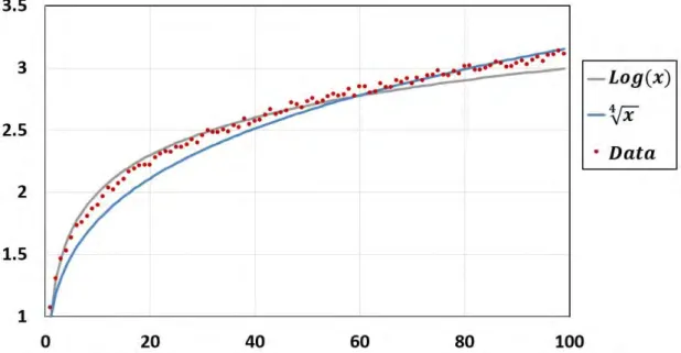
Structural uncertainty usually represents the lack of confidence that the structure of the constructed model reflects adequately the studied real system. In such cases, a modeler could not be sure that the output would be correct, even if the true values of all the inputs and parameters are known. To clarify this type of uncertainty, consider for example the case study of having the corresponding data points of a studied system and the aim is to find its structure. As shown in Fig. 1.1, the data points can be fitted by a logarithmic function and by a 4th root function. In this case it is not sure which formula is the true representation of the model, and hence there is a structural uncertainty.

Figure 1.1: The data fitted to a logarithmic function and to a 4th root function.

During modeling, several factors may lead to structural uncertainty. One of these factors is the simplifications and scientific judgments made when constructing and interpreting the model. Other factors are the incomplete understanding of the system under study and the inappropriate equations used to express this system. Even though these causes were taken in consideration, the definite elimination of structural uncertainty was impos-sible, however the emphasis was to reduce this uncertainty as much as possible. Methods of structural uncertainty assessment try to find the optimal model structure that best represents the real studied system.

(24)

1.3 Structural uncertainty assessment

models are built representing all the possible emulations of the true structure. Then a strategy is used to derive the aspect of the final model from the set of possible models. Model Selection [Leeb et Pötscher, 2005] and Model Averaging [Strong et al., 2009] are the two most popular and broad approaches used in this context. In Model Selection, an optimal model from the set of models is selected according to some criteria provided by experts. Some criteria that are proposed in [Bojke et al., 2009] include Residual Mean Squared Error, Finite-Prediction-Error, Minimum Variance Criteria, and subjective prob-abilities. On the other hand, in Model Averaging, instead of choosing one single model, the weighted average of the proposed models is taken. In this case, a suitable weight is assigned to each plausible model according to how much it matches reality.

Another method to cope structural uncertainty more flexibly is known as "Parameteriza-tion of structural uncertainty" [Strong et al., 2012]. The idea is to describe the uncertainty of the model by introducing new uncertain parameters, for instance correction factors, boolean elements, or exogenous variables. Thus a single general model is constructed in such a way that every other plausible model is considered as a particular case of this general model. In such a situation, the general model is considered to be studied under the effect of only input uncertainty with no structural uncertainty.

Although these strategies seem straightforward and really helpful in reducing and study-ing structural uncertainty, they still have some limitations. Indeed, usstudy-ing Model Selection may be disadvantageous in several cases. This is because selecting one model will prob-ably discard important eventualities from other alternative models. On the other hand, the Model Averaging strategy allows the collection of all possible models, however, when using large models with with highly computational cost, it becomes difficult to find the average. Parameterization of structural uncertainty is practical when dealing with struc-tural uncertainty, however not all strucstruc-tural uncertainties are that easy to be represented by a parameter. As a conclusion, a modeler should be cautious while choosing the appro-priate approach to reduce the structural uncertainty.

In this section, a general idea about methods that deal with structural uncertainty was presented. Although different methods exist in this manner, but none of them can guar-antee that the true model can be attained. Thus the goal was to achieve the best level of confidence while choosing the structure of the model.

(25)

In the following sections, we continue with the methods of uncertainty quantification and sensitivity analysis, which are the main focus of our work. However in the sequel we will assume that we are dealing with an exact true model that has no structural uncertainty.

1.4 Input uncertainty representation

For the sake of clarity, it is important to note that methods that study input uncertainty rely first on finding a representation of the uncertainty. Several ways have been proposed. However, the most practical and used one is the probabilistic way. In the following para-graph, in each method of uncertainty quantification and sensitivity analysis the associated representation way of uncertainty will be introduced. In exception, the probabilistic way is introduced here since its notion is used in most methods and in Chapter 2.

The uncertainty at an input point a = (a1, · · · , an) is represented probabilistically by a

random vector (vector of random variables) which will be denoted by X = (X1, · · · , Xn).

Each Xi represents the uncertainty at ai. The uncertainties at ai’s are assumed to be

independent, and hence the random variables X1, · · · , Xn are mutually independent. The

realizations of each random variable Xi are the uncertain values xi supplied to F that are

supposed to be equal to ai. These realizations are collected in a set denoted by Ωi. Then

the collection of the realizations of the random vector x is the set Ω = Ω1× · · · ×Ωn.

To clarify this notation of uncertainty consider the following example. Let

F(x1, x2) = πx1x22 (1.2)

be the function that gives the volume of some liquid in a cylinder. The first input x1

represents the height attained by the liquid in the cylinder in mm, and the second input

x2 represents the radius of the cylinder also in mm. Suppose that for a certain liquid the

values of x1 and x2 are 9.762 and 3.91 respectively, but these true exact values are not

known. Thus to get the volume of the liquid, measurements for x1 and x2 should be done.

The measurement process is pictured in Fig. 1.2.

Note that with the measurements of Fig. 1.2 we can not be sure about the exact values of x1 and x2 for the given liquid. This implies that there is input uncertainty for both

(26)

1.4 Input uncertainty representation

Figure 1.2: The measurements of the height x1 and the radius of the cylinder x2.

variables x1 and x2. Let X1 be the random variable representing the uncertainty at x1,

and let X2 be the random variable representing the uncertainty at x2. Then the input

uncertainty of F at the point (9.762, 3.91), which we suppose is not known, is represented by the random vector (X1, X2). Note that the realizations of the random vector X1 are

all the possible true values for x1 and they are collected in a set Ω1. Similarly for X2,

its realizations are all the possible true values of x2 and they are collected in a set Ω2.

From Fig. 1.2, one can define the sets Ω1 and Ω2 by Ω1 = [9.5, 10] and Ω2 = [3.5, 4]. We

associate here intervals to the sets Ω1 and Ω2 since x1 and x2 take real values. So any

real value between 9.5 and 10 is a possible true value for x1, and this gives an interval,

and similarly for x2 its possible true values are collected in an interval.

Actually what we present here is a very simple example of uncertainty that one may face. However in big problems, uncertainty could be much more complicated and it cannot be eliminated even with highly accurate measurements.

Now we continue with the probabilistic representation of the input uncertainty. Each random variable Xi, as a representation of the input uncertainty, is associated with a

probability distribution which specifies the probability of each possible value xi to be the

true value ai. Here we distinguish two cases:

(27)

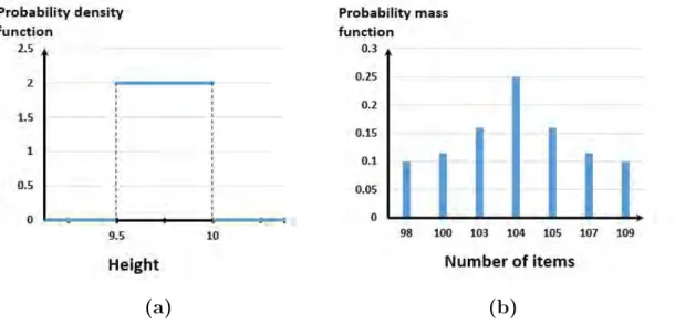
case, is the uncertainty presented in the inputs of the example of Fig. 1.2. Realizations in this example are real numbers taken between two limits and Ωi is an interval, thus

it is not finite. In this case each Xi is characterized by a probability density function.

Fig. 1.3(a)shows the probability density function of the height presented in the example above.

2. If Ωi is finite, Xi is a discrete random variable and its probability distribution is

charac-terized by a probability mass function. An example of this discrete case, is an uncertainty in an input which represents the number of items sold by a store per year. Realizations in this example are natural numbers and could not be real numbers, and so the Ωi is for

sure finite. In this case the random variable is characterized by a mass function (see Fig.

1.3(b)).

(a) (b)

Figure 1.3: Probabilistic presentation of input uncertainty: (a) continuous distribution,

(b) discrete distribution .

Usually input uncertainty is represented by a discrete random variable if the input itself represents a number of something, like items, so that the input takes only natural numbers (or integer values). In this case, the realizations of the associated random variable are integer values and hence the associated set of possible values is definitely finite. However continuous random variables are used to represent the input uncertainty for inputs taken from measurement or experiments. In this case, the possible true values are real numbers forming an infinite set, and in fact this is the most popular case.

(28)

1.4 Input uncertainty representation

the techniques presented are equally applicable for discrete distributions. The probabil-ity densprobabil-ity functions of X1, · · · , Xn are denoted by p1(x1), · · · , pn(xn). Accordingly, the

probability distribution of the random vector X is pX(x) = Qni=1pi(xi).

Usually, the probability distributions of the random variables are selected based on either prior data or subjective judgments of experts. In [Hammonds et al., 1994], the authors proposed some simple guidelines to derive the appropriate continuous distribution. These guidelines state that when the data are limited and the uncertainty range is relatively small, a uniform distribution can be used and the associated support interval is charac-terized by the uncertainty range. If there is more knowledge about a most likely value or midpoint, in addition to the range of the uncertainty, a triangular distribution may be assigned. When the range of the uncertainty is very large, a log-uniform or log-triangular distribution may be more appropriate than the uniform or the triangular distribution. The assumption of normal, log-normal, or empirical distributions usually depends on the availability of the relevant data, where a fitting process is usually used to guess such probability density functions. In addition to this, the authors in [Hammonds et al., 1994] indicated that other continuous distributions can be also used such as Gamma, Beta, and Poisson. Note that, analogous guidelines can be derived for the discrete case.

With this probabilistic representation of the input uncertainty at a, the corresponding output uncertainty at F (a) is represented by a random variable denoted by Y . This random variable is defined as Y = F (X1, · · · , Xn), and its probability density function is

denoted by pY. Note that the random variable Y and the random variables X1, · · · , Xn

are dependent, as y is a function of the other random variables.

The best estimate of the true value of a is given by the mean of X which will be denoted by µX = (µ1, · · · , µn). Similarly, the best estimate of the true value of F (a) is given by

the mean of Y which will be denoted by µY.

Concerning the quantity of uncertainty at a, it is usually represented by the variance of

X, denoted by V = (V1, · · · , Vn). However, for some specific distributions, other

sta-tistical parameters can be used to represent the quantity of uncertainty. For instance, for a uniformly distributed random variable, the radius of the support vector could be used to represent the quantity of uncertainty since it gives the dispersion of the values around the expected value. Similarly, the quantity of the output uncertainty is usually

(29)

represented by the variance, which will be denoted by V ar(Y ). However, the quantity of the output uncertainty can also be represented by other statistical parameters depending on the associated distribution. In the following , whenever the probabilistic point of view is used to represent uncertainty, the representative of the quantity of the uncertainty will be stated explicitly.

1.5 Forward uncertainty propagation

Forward Uncertainty Propagation is performed to investigate the uncertainty in the model’s output that is generated from the uncertainty in the model’s input [Marino et al., 2008]. The idea is to associate a representation for the input uncertainty, then accordingly try to find the output uncertainty in the same representation type. Methods in this group are classified as either probabilistic and non probabilistic, according to the way the input uncertainty is represented. Probabilistic methods use the probabilistic point of view to represent the input uncertainty (see section 1.4). Then through propagation, the proba-bilistic presentation of the model output is to be determined. Mainly, we seek the mean

µy and the variance V ar(Y ) of the the random variable Y which represents the output

uncertainty. The non probabilistic methods, however, use a non probabilistic forms to represent the input uncertainty. Then, according to the used form, the associated output representation is to be determined. In the following two subsections, classical methods from both categories are presented.

1.5.1 Probabilistic methods

In the probabilistic uncertainty propagation methods, each uncertain input is represented by a random variable and it is specified by a probability density function. Then, model output, as a function of the model input, is also a random variable whose statistical mo-ments are to be determined. Fig. 1.4 illustrates the probabilistic mode of the forward propagation of uncertainty.

The main concern is to find the first and the second moments of the output i.e. the mean and the variance. This task is devoted mainly to the propagation techniques.

(30)

Dif-1.5 Forward uncertainty propagation

Figure 1.4: Probabilistic propagation of input uncertainty.

ferent techniques are widely known in this manner, and the following is a summarized explanation of three of them. The first is called Monte Carlo, which is a simulation based technique. The second, generally known as Spectral Method, is based on functional expansion. The last one is the Perturbation Method, which is a local expansion based method.

Monte Carlo

Monte Carlo is one of the oldest and most popular simulation based methods in uncer-tainty propagation. It is used in order to estimate the mean value µY and the variance

V ar(Y ) as well as the probability density function of Y . First, M samples of input data

values {xk _{= (x}(k)

1 , · · · , x(k)n )}k=1···M are drawn randomly from the distributions of Xi,

according to their probability density functions. These sample points are then run by the model F to obtain their corresponding output values. The obtained values of the output are then collected to find its statistical characteristics. For instance, the computation of the expectation and variance of the output Y is done using the approximation formulas:

µY = 1 M M X k=1 F(X(k)) (1.3) V ar(Y ) = 1 M −1 M X k=1 (F (X(k)_{) − µ} Y)2 (1.4)

On the other hand, the distribution of Y can also be derived simply by using the obtained output data in a fitting process.

(31)

applicable and does not require any assumptions on the model form as linearity or con-tinuity. Moreover, the number of sample points M needed in the simulation is generally independent of n, the size of the input vector x [Helton et Davis, 2002]. However, it is important to note that the method converges to the exact stochastic solution as the number of samples goes to infinity, so thousands or millions of samples may be required to obtain accurate estimations [Iaccarino, 2009]. This could be problematic in the case of computationally expensive models and/or in the case of important size of input vector. Several methods have been developed to accelerate the convergence of the Monte Carlo approach. Indeed, in the basic Monte Carlo simulation, random sampling is used. How-ever by using other sampling techniques, a faster convergence can be achieved. Examples of such sampling techniques are: stratified sampling, Latin Hyper cube sampling, sam-pling based on Sobol’s sequences [Burhenne et al., 2011]. For instance, in Latin Hyper cube sampling the range of each input random variable Xiis divided into M equiprobable

intervals. Then, M random samples are drawn, by collecting for each sample one element from each of the equiprobable intervals. Thus each sampled point is associated with one of the rows and one of the columns. This ensures more coverage of the range of the inputs than the case of just random sampling. Fig. 1.5 shows the difference between the random sampling (basic Monte Carlo) and the Latin Hyper cube sampling for eight samples for two inputs.

(a) (b)

Figure 1.5: Scatter plot of sampling techniques: (a) Random sampling, (b) Latin Hyper cube sampling.

In Fig. 1.5, the Latin Hyper cube sampling shows some gaps and clusters like the random sampling because the sample size is too small. Note that as the number of samples

(32)

in-1.5 Forward uncertainty propagation

creases, the number of rows and columns increases, and hence there will be more coverage of the range of inputs.

To conclude, the Monte Carlo method is a practical method for propagating uncertainty, however its performance depends on the number of samples available. With the devel-opment of high performance software, computation of big samples becomes more easy. However it remains a problem for the models with high computation cost.

Spectral Methods

Spectral methods represent an alternative strategy for uncertainty propagation. Their basic idea is to write the model as an infinite sum of some basis functions. Indeed, this expansion eases the derivation of the moments (mean and variance) of the output random variable Y . Different basis functions have been used for such expansion, depending on the distribution of the input random variables X1, · · · , Xn. However the most used basis are

polynomials. Several approaches with different polynomial basis have been used [Gilli, 2013]. The most known one in this manner is the Polynomial Chaos Expansion (PCE), defined using multidimensional orthogonal polynomials as representative basis. Here, we give a general overview about the Polynomial Chaos Expansion, considering it as a typical illustration of the expansions of the spectral methods.

The first proposed Polynomial Chaos expansion employed the Hermite polynomials in terms of Gaussian random variables to generate the expanded series. According to [Lee et Chen, 2009], its expression is:

u= a0H0+ ∞ X i1=1 ai1H1(φi1) + ∞ X i1=1 i1 X i2=1 ai1i2H2(φi1, φi2) + ∞ X i1=1 i1 X i2=1 i2 X i3=1 ai1i2i3H3(φi1, φi2, φi3) + ... (1.5)

for an arbitrary random variable u, where {φi1}

∞

i=1 is a set of standard normal variables,

Hi is a generic element in the set of multidimensional Hermite polynomials of order i, and

ai are coefficients to be determined. For convenience, the expression was rewritten in a

more compact way:

u=

∞

X

i=0

(33)

where bi and Ψi(φ) correspond to ai1i2...ip and Hp(φi1, φi2, ..., φip) respectively. Note that the orthogonality property with respect to the standard normal probability density func-tion of the Hermite polynomials implies that

E[ΨiΨj] = E[Ψ2i]δij and E[Ψi] = 0 for i 6= 0 (1.7)

where E represents the expectation. Hence, the set {Ψi}forms an orthogonal basis of the

space of functions having normally distributed variables.

In practice, when there are n uncertain inputs standard normally distributed, the output response can be approximated by n-dimensional PCE, truncated at some order p [Lee et Chen, 2009]. In this case, the number of terms in PCE becomes P + 1 where P is given as P = p X s=1 (n + s − 1)! s!(n − 1)! (1.8)

Thus, the model output approximation is given by ˜Y =XP

i=0

biΨi(X) (1.9)

with X = (X1, X2, ..., Xn). The derivation of the coefficients can be carried out

analyti-cally [Schick, 2011], otherwise by utilizing sampling or projection techniques [Le Maître et Knio, 2010].

Since the above procedures are only compatible with standard normal variables, the way of treating other random variables became an important issue. To cope with this prob-lem, a generalized PCE was proposed based on different polynomial basis, where each corresponded to a set of orthogonal polynomials related to the underlying probability density function of the random vector. With the generalized PCE, non-normal distribu-tions such as beta, gamma, and uniform distribudistribu-tions could be used as a standard input vector [Lee et Chen, 2009]. Accordingly, Gaussian variables ware best approximated by Hermite polynomials. Legendre polynomials accounted for the best approximation of a uniformed distributed variable, whereas Jacobi polynomials should be used for Beta dis-tributions [Sepahvand et al., 2010].

(34)

1.5 Forward uncertainty propagation

variables can be involved in the same expansion. Thus, later, the approach was extended by assuming that the input vector components are independent distinct random variables, where a multi-dimensional basis is constructed as a simple product of the corresponding constructed one dimensional orthogonal polynomials.

Once the expansion of the model function is obtained, the moments (mean and variance) of the output can be derived. While the accuracy of the generalized PC approach can be improved by increasing the polynomial order of truncation, it should also be noted that as the number of inputs and the expansion order increase, the number of unknown co-efficients to be determined increases exponentially, thereby increasing the computational costs [Kewlani et al., 2012]. Thus this method is suitable for models with a small number of uncertain inputs.

Perturbation Method

The Perturbation method is an alternative way for uncertainty propagation, based on local expansion of the model function [Sudret, 2007]. The idea is to consider the trun-cated Taylor expansion of the model F in the neighborhood of µX the mean of the input

random vector X: F(X) = F (µX) + n X i=1 ∂F ∂Xi _X=µ(Xi− µi) +1₂Xn i=1 n X j=1 ∂2F ∂Xi∂Xj _X=µ(Xi− µi)(Xj− µj) + o(k X − µX k 2₎ (1.10)

Then the expectation of Y is:

µY = E[Y ] = E[F (X)] ≈ F (µ) + n X i=1 ∂F ∂Xi _X=µE[(Xi− µi)]+ n X i=1 N X j=1 ∂2_F ∂Xi∂Xj _X=µE[(Xi− µi)(Xj − µj)] (1.11)

Note that E[(Xi − µi)] = 0 for every i, and E[(Xi − µi)(Xj − µj)] = Cov(Xi, Xj).

(35)

Cov(Xi, Xj) = 0 for all i 6= j. Hence, the expectation of Y is simplified into: µY = E[F (X)] ≈ F (µ) + n X i=1 ∂2_F ∂2_X i _X=µ Vi (1.12)

As it can be seen, the expectation of the uncertain output is approximated by two terms. The first term is F (µX), the value of the model F at the mean of the uncertain input,

which is called the first order approximation of µY. The second term is a second order

correcting term which depends on the variances of the inputs and the partial derivatives of the model form F . In a similar manner, the variance of Y can be approximated. So starting from the formula:

V ar(Y ) = E[(Y − E(Y ))2] ≈ E[(Y − F (µ))2] (1.13)

Using the Taylor expansion, then V ar(Y ) is approximated by:

V ar(Y ) ≈ E     n X i=1 ∂F ∂Xi _X=µ(Xi − µi)   2  ≈ n X i=1 n X j=1 ∂F ∂Xi _X=µ ∂F ∂Xj _X=µE[(Xi− µi)(Xj − µj)] (1.14)

As E[(Xi− µi)(Xj− µj)] = 0 for all i 6= j, V ar(Y ) ends up with:

V ar(Y ) ≈ n X i=1   ∂F ∂Xi X=µ   2 Vi (1.15)

An interpretation of this approximation implies that the variance of the response is the sum of contributions of each input, where each contribution is a mix of the variance of this input and the gradient of the response with respect to this input.

This method appears quite general and it is applied at a low computational cost, espe-cially if the gradient of the model response is available. However, it can be applied only for models with small uncertainties, due to the local nature of the Taylor expansion ap-proximation.

(36)

uncer-1.5 Forward uncertainty propagation

tainty propagation, is the same as choosing between high accuracy and less cost. Spectral methods rely on complete expansion of the model while the perturbation method relies on the local expansion of the model. The first costs more, but give more accurate results than the second. Thus in applications one should compromise between cost and accuracy. In this subsection, three different uncertainty propagation methods were revised. The common point between these methods is that they rely on the probabilistic representa-tion of uncertainty. Their main goal is to find the probabilistic moments of the output uncertainty. This is done either numerically by simulation (Monte Carlo method) or by using an expansion of the output formula (spectral and perturbation methods). In gen-eral, these methods are considered simple from a theoretical point of view. In the next section, non probabilistic methods for uncertainty propagation are presented. The con-cept of some of these methods may be considered as generalization of the probabilistic approach, however some other methods have completely different notions.

1.5.2 Non-Probabilistic methods

As discussed in the previous section, the probabilistic uncertainty propagation methods are usually applied when the information about the uncertain inputs are sufficient to con-struct a probabilistic distribution. However, if the information of the uncertain element is insufficient, the non-probabilistic approaches can be used [Gao et al., 2011]. Below, alternative approaches to the probabilistic approach of uncertainty presentation are dis-cussed, including Interval theory, Fuzzy theory, Possibility theory, and Evidence theory. The way the uncertainty is propagated using these uncertainty presentation approaches is also discussed.

Interval Analysis

Interval analysis [Moore et al., 2009] is one of the simplest ways to propagate uncertainty in data-poor situations. In interval analysis, it is assumed that nothing is known about the uncertain input except that it lies within certain bounds. Each uncertain input is represented by an interval. An interval here refers to a close set in R, which includes the

(37)

where the real numbers a and b are the lower and upper limits of the interval. According to the author of [P Swiler et al., 2009], the problem of uncertainty propagation can be turned into an interval analysis problem: given the inputs’ uncertainties represented by intervals, what is the corresponding interval of the output uncertainty?

The interval of the output uncertainty is determined by finding the infimum and supre-mum attained by the model when the uncertain inputs vary entirely over their associ-ated intervals. When the model is a simple expression with simple arithmetic operations (+, −, ×, ÷), then the output interval is determined by extending these elementary arith-metic operations to intervals. Such extension is as follows

I op J = {c op d such that c ∈ I, d ∈ J} (1.16)

where I and J are two intervals, and op refers to one of the arithmetic operations. How-ever, the determination of the output interval becomes much more complicated if the model has a complex form. Non linear optimization problems might be used to determine the upper and the lower limits of the output interval. This probably requires a large number of model evaluations. Furthermore, most optimization solvers are local, and thus the global optima is not guaranteed. Which means that it is not easy to find the infimum and supremum. Hence, to solve interval analysis problems properly, global methods must be used, and usually these approaches can be very expensive.

In brief, interval analysis is suitable for propagating uncertainty in problems where the model has an elementary form, with a small number of inputs.

Fuzzy Set Theory

Another approach to represent the uncertainty of the input is the Fuzzy Set Theory. In the Fuzzy Set Theory, an uncertain input is treated as fuzzy number, and its correspond-ing uncertainty is characterized by membership functions. Such membership functions associate a weight between 0 and 1 to every possible value of the uncertain input. Then, to propagate the input uncertainty and find the output uncertainty, the output member-ship function is to be determined. To this end, some procedures are carried. Here, we give a quick review of the notions of the Fuzzy Set theory as it is used in uncertainty propagation.

(38)

The starting point will be the definition of the widely used term "Fuzzy Set". Let U be a universe set of τ values (elements), set A is called a fuzzy set if it is composed of ordered pairs in the following form:

A= {(τ, ΦA(τ)) | τ ∈ U, ΦA(τ) ∈ [0, 1] } (1.17)

where ΦA(τ) is the degree of membership of τ in A. The function ΦA is called the

mem-bership function of A.

A special case of fuzzy sets are the so-called fuzzy numbers. According to [Schulz et Huwe, 1999], a Fuzzy number A is a fuzzy set satisfying the following :

1. The membership function ΦA is piecewise continuous, and the elements τ are real

numbers, i.e. A = {(τ, ΦA(τ)) | τ ∈ U ⊆ R, ΦA(τ) ∈ [0, 1] }.

2. A is normal, i.e. there exists at least one (τ, ΦA(τ)) ∈ A such that ΦA(τ) = 1.

3. A is a convex set, i.e. for any (τ1,ΦA(τ1)), (τ2,ΦA(τ2)), and (τ3,ΦA(τ3)) ∈ A, the

following implication holds:

τ1 < τ3 < τ2 ⇒ΦA(τ3) ≥ min{ΦA(τ1), ΦA(τ2)} (1.18)

This simple concept of fuzzy numbers permits its application in the domain of uncertainty propagation. Indeed, an uncertainty at one real valued input point ai of point a =

(a1, · · · , an) is represented by a fuzzy number Ai with a specific membership function

Φi. The elements τ of Ai are the uncertain values supplied to F that are supposed to be

equal to ai. The membership function Φi is usually constructed based on the available

information about the uncertain input. In this manner, a general followed guidance is: the closer Φi(τ) is to 1, the more the element τ is accepted as a true value for ai, and

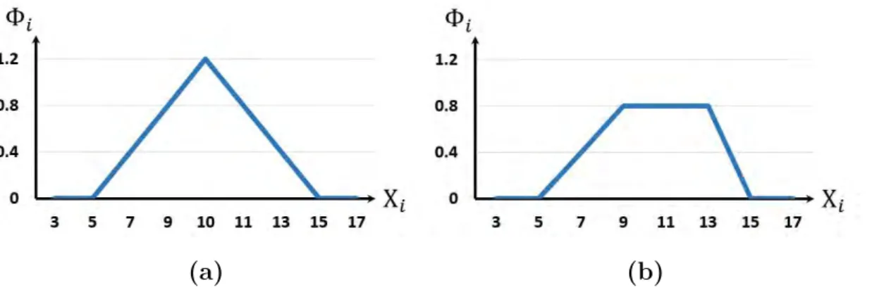
the closer it is to 0, the less it is accepted. Several forms of the membership function of a fuzzy numbers has been developed and used in the domain of uncertainty [Wierman, 2010], including triangular and trapezoidal shaped membership functions. Illustrations

(39)

of such membership functions are given in Fig. 1.6 to represent the uncertainty of a measured quantity around the value 10.

(a) (b)

Figure 1.6: Fuzzy membership functions: (a) Triangular, (b) Trapezoidal.

After associating to each uncertain input a fuzzy number, the propagation of uncertainty is performed using the extended principle of fuzzy set theory [Maskey et al., 2004]. According to this principle, the membership function of the output y is given by:

Φy(y) =        sup{min(Φ1(x1), · · · , Φn(xn)) y = f(x1, ..., xn)

0 if no (x1, · · · , xn) exist such that f(x1, · · · , xN) = y

(1.19)

Thus, the uncertain output is represented by a fuzzy number {(y, Φy(y))}. Its

member-ship function is determined at each possible value y of F (a) by applying the formula (1.19). This indicates the spread of the output uncertainty as well as the most probable true value F (a).

This method of uncertainty propagation has been applied in various domains, examples are in [Schulz et Huwe, 1999;Maskey et al., 2004], where usually the number of uncertain parameters is small, or the model form is monotone with respect to the inputs. In cases where more complex models have to operate on fuzzy numbers, the above procedure re-sults in nonlinear numerical optimization problems at each possible value of the output, and hence this would be computationally expensive.

The Dempster-Shafer Theory

The Dempster-Shafer Theory(DST), also known as evidence theory, is an uncertainty propagation method used when the available information is mostly provided by experts.

(40)

Unlike probability theory, in DST there are two measures of likelihood and not a single probability distribution function. These two measures are called belief and plausibility. The following paragraph is a description of the derivation of such measures as well as their role in uncertainty propagation. Readers interested in more details about DST are referred to [Baraldi et Zio, 2010].

As a first step for quantifying the input uncertainty in DST, a finite set Ωi is assigned

to each uncertain input xi at the uncertain point ai consisting of all the uncertain values

supplied to F that are supposed to be equal to ai. Then a mass function is associated

with each set Ωi, called the Basic Belief Assignment (BBA) and denoted by Bi. The BBA

is a mapping Bi : P(Ωi) 7−→ [0, 1] satisfying:

Bi(φ) = 0 and

X

A⊂Ωi

Bi(A) = 1 (1.20)

where P(Ωi) is the power-set of Ωi i.e. the set of all subsets of Ωi. For every A ⊂ Ωi,

the value Bi(A) indicates how likely the true value of the uncertain input falls within the

subset A. Each A ⊂ Ωi with Bi(A) > 0 is called a focal element of Bi. Note that, as

P

A⊂ΩiBi(A) = 1, the BBA function has a finite number of focal elements. Moreover, a BBA function is completely defined by these focal elements and their associated masses according to [Limbourg, 2008].

In DST, the function Bi is not the fundamental measure of likelihood. Rather, this BBA

is used to derive the two measures of likelihood: the belief and the plausibility. According to [Helton et al., 2004], the belief, Bel(A), and the plausibility, P l(A), for a subset A ⊂ Ωi

are defined by:

Beli(A) = X C⊆A Bi(C) (1.21) and P li(A) = X C∩A6=∅ Bi(C) (1.22)

Observe that these two summations can be simply computed since Bi has a finite number

of focal elements. Further more, the belief Beli(A) is commonly considered as a lower

bound of the probability that the true value of xi is within A. On the other hand, the

Methods for sensitivity analysis and backward propagation of uncertainty applied on mathematical models in engineering applications

HAL Id: tel-01945221

https://tel.archives-ouvertes.fr/tel-01945221

models in engineering applications

Iman Alhossen

To cite this version:

THÈSE

En vue de l’obtention du

DOCTORAT DE L’UNIVERSITÉ DE TOULOUSE

Délivré par:

Université Toulouse 3 Paul Sabatier (UT3 Paul Sabatier)

Présentée et soutenue par :

Iman ALHOSSEN

le 11 Décembre 2017

Titre :

Méthode d’analyse de sensibilité et propagation inverse d’incertitude

appliquées sur les modèles mathématiques dans les applications d’ingénierie

École doctorale et discipline ou spécialité :

ED MEGEP : Génie mécanique

Unité de recherche :

Institut Clément Ader, CNRS UMR 5312

Directeur(s) de Thèse :

Stéphane Segonds

MCF (HDR), Université Paul Sabatier

Directeur

Florian Bugarin

MCF, Université Paul Sabatier

Co-Directeur

Jury :

Bertrand Wattrisse

PR, Université de Montpellier

Rapporteur

Mhamad Khalil

PR, Université Libanaise

Rapporteur

Adrien Bartoli

PR, Université Clermont Auvergne

Président

Cyril Bordreuil

PR, Université de Montpellier

Examinateur

Fulbert Baudouin

MCF, Université Paul Sabatier

Examinateur

Acknowledgment

Abstract

Résumé

Contents

List of Figures

List of Algorithms

1

Literature Review

Contents

1.1

Introduction

1.2

General notation of a model

1.3

Structural uncertainty assessment

1.4

Input uncertainty representation

1.5

Forward uncertainty propagation

1.5.1

Probabilistic methods

1.5.2

Non-Probabilistic methods