HAL Id: hal-00639681
https://hal.inria.fr/hal-00639681
Submitted on 9 Nov 2011
HAL is a multi-disciplinary open access
archive for the deposit and dissemination of
sci-entific research documents, whether they are
pub-lished or not. The documents may come from
teaching and research institutions in France or
abroad, or from public or private research centers.
L’archive ouverte pluridisciplinaire HAL, est
destinée au dépôt et à la diffusion de documents
scientifiques de niveau recherche, publiés ou non,
émanant des établissements d’enseignement et de
recherche français ou étrangers, des laboratoires
publics ou privés.
Vision based control for Humanoid robots
Claire Dune, Andrei Herdt, Eric Marchand, Olivier Stasse, Pierre-Brice
Wieber, Eiichi Yoshida
To cite this version:
Claire Dune, Andrei Herdt, Eric Marchand, Olivier Stasse, Pierre-Brice Wieber, et al.. Vision based
control for Humanoid robots. IROS Workshop on Visual Control of Mobile Robots (ViCoMoR), Sep
2011, San Francisco, USA, United States. pp.19-26. �hal-00639681�
Vision based control for Humano¨ıd robots
C. Dune, A. Herdt, E. Marchand, O. Stasse, P.-B. Wieber, E. Yoshida
Abstract— This paper presents a visual servoing scheme to control humanoid dynamic walk. Whereas most of the existing approaches follow a perception-decision-action scheme, we hereby introduce a method that uses the on-line information given by an on-board camera. This close looped approach allows the system to react to changes in its environment and adapt to modelling error. Our approach is based on a new reactive pattern generator which modifies footsteps, center of mass and center of pressure trajectories at the control level for the center of mass to track a reference velocity. In this workshop, we present three ways of servoing dynamical humano¨ıd walk : a na¨ıve one that compute a reference velocity using a visual servoing control law, a second one that takes into account the sway motion induced by the walk and an on going work on vision predictive control that directly introduces the visual error in the cost function of the pattern generator. The two first approaches have been validated on the HRP-2 robot. These close loop approaches give a more accurate positioning than the one obtained when executing a planned trajectory especially when rotational motion are involved.
I. INTRODUCTION
Humanoid robots are designed for human environments, defined as unstructured and dynamic environments [1] where objects move outside robots’control. In order to complete a specific task, humanoid robots must perceive and react to en-vironmental changes. Vision based control may help them to perceive their surroundings in order to adapt their behaviour efficiently. Indeed, most of the humanoid robots are equipped with cameras that provide rich information without adding so much weight and size. The use of embedded camera is attractive because it avoids equipping the environment with additional sensors, and thus the system is more autonomous. Yet, extracting data from these cameras is a real challenge, especially while walking.
In this paper, we introduce a monocular visual servoing scheme to control the HRP-2 walk towards an object with taking into account the peculiar motion of the on-board camera induced by the stepping.
A. State of the art
Previous works on humanoid walking control assume that the robot path is defined before computing the actual joint C. Dune was with CNRS-AIST, JRL (Joint Robotics Laboratory), UMI 3218/CRT, Intelligent Systems Research Institute, AIST Central 2, Umezono 1-1-1, Tsukuba, Ibaraki 305-8568 Japan and is now with Handibio, EA4322 Universit´e du Sud- Toulon Var.
O. Stasse and E. Yoshida are with CNRS-AIST, JRL (Joint Robotics Laboratory), UMI 3218/CRT, Intelligent Systems Research Institute, AIST Central 2, Umezono 1-1-1, Tsukuba, Ibaraki 305-8568 Japan
A. Herdt and P.-B. Wieber are with Bipop team Inria Rhˆone Alpes, Grenoble, France
E. Marchand is with Lagadic team Inria Rennes Bretagne Atlantique, Rennes, France
control to realize it. They generally follow a perception-decision-action scheme: first, a sensor acquires data on the world and/or the robot state, then, suitable footsteps over a time horizon are decided, and the trajectories of the center of mass (CoM) and the center of pressure (CoP) are com-puted while respecting the stability constraints. Finally, the control of the legs is computed by inverse kinematics. This perception-decision-action loop has proven to be fast enough to realize impressive demonstrations for stair-climbing and obstacle avoidance [2], [3], [4], [5]. Object cM k x y z z Side view K C F ! k∗ Mo ! kM o
Fig. 1. The robot has to reach a desired position with regards to an object
We claim that a visual servoing control scheme is well suited for vision based walking motion generation because it compensates for model errors. Visual servoing proved to be successful for grasping tasks with standing [6], [7] or walking humanoids [8], [9]. In [8], visual servoing is used to control a humanoid avatar along landmarks. The upper body is approximated by the kinematic chain that links an on-board camera to the CoM. The lower body is controlled by adding two translational degrees of freedom to the CoM. The translational velocity of the CoM is sent to a kinematic locomotion module which control the legs motion. In [9] a whole body visual servoing scheme based on a hierarchical stack of task is introduced. However, the footsteps are predefined. The leg motion is thus set to be the task of higher priority. Therefore visual-servoing in this context is projected in the null-space of the pre-defined walking path. On the contrary in this work, the controller driving the walk is directly guided by vision.
Few work deal with footsteps, CoM and CoP trajectories modification inside the preview window. The work presented
IROS Workshop on Visual Control of Mobile Robots (ViCoMoR) September 26, 2011, San Francisco, California, USA
in [10] shades some light on this problem. It shows that modifying the next landing position of the flying foot might impose a new CoP trajectory going out of the support polygon. This can jeopardize the equilibrium of the robot. To solve the problem, the stepping period may be modified to reduce this instability [10], at the cost of slowing down the robot. A recent method proposes to modify the footsteps according to a perturbation applied to the CoP [11]. In the current paper the desired velocity computed by a visual servoing based controller is directly used to change footsteps, while ensuring walking stability constraints and with time intervals of constant length. Another difference lays on the fact that, on the one hand, the CoP is constrained at the center of the footprints, and on the other hand the CoP can move freely inside the support polygon.
B. Contribution
Our approach is based on a new pattern generator (PG) that has been proposed by Herdt et al [12], [13]. It computes a reactive stable walking motion for the CoM to track an instant reference velocity without predefined footsteps. This paves the way to reactive walking motion based on current environmental perception.
In this paper, we introduce a real time vision based control of HRP-2 walking motion. It is based on the visual servoing scheme we introduced in [14] applied to a positioning task. This scheme has the advantage of handling both fixed and mobile object. The only requirement is to know at least partially the 3d model of the object : some 3d edges for angular objects or the diameter of a sphere for a ball.
C. Paper overview
Section II is dedicated to the new PG description. Section III presents the model based tracker and the visual servoing control and Section IV presents the results obtained using our approach with regards to the execution of a planned trajectory. Section V draws the conclusion and perspectives.
II. PREDICTIONCONTROLSCHEME FORREACTIVE WALKINGMOTION
This section presents the on-line walking motion generator introduced in [12], [13]. The robot is modelled as a linear inverse pendulum which fits fairly well with the HRP-2 distribution of mass. The control is based on a Linear Model Predictive Control scheme that computes the footsteps and the optimal jerk of the point mass model to minimise the difference between a reference CoM velocity and the previewed one.
A. Systems Dynamics
The humanoid robot is modelled as an oriented mass point centred on the robot CoM. This paragraph describes the dynamics of a stable walking motion.
1) Motion of the Center of Mass: Let us consider a frame C attached to the position of the CoM of the robot and to the orientation of its trunk. The position and orientation of this frame will be noted c = "cx cy cz cϕ cψ cθ#,
with Cardan angles cϕ,cψ andcθ.
The acceleration ¨c of this frame has to be continuous for being realized properly by usual actuators. We will consider here that it is in fact piecewise linear on time intervals of constant length τ , with a piecewise constant jerk ...c (third derivative of the position) on these intervals. The trajectory of this frame over longer time intervals of length nτ can be simply obtained by integrating over time the piecewise constant jerk together with the initial speed˙c and acceleration ¨
c. For any coordinate α ∈ {x, y, z, ϕ, ψ, θ}, this leads to simple linear relationships
Cα i+1= Spcˆαi+ U p ... Cαi, (1) ˙ Cα i+1= Svˆcαi + Uv ... Cαi, (2) ¨ Cα i+1= Sacˆαi + Ua ... Cαi, (3)
where the initial state is cˆα
i = " cα(t i) ˙cα(ti) ¨cα(ti) #T , andCα
i+i is the vector of the state on the prediction horizon
that can is defined by
Cα i+1= cα(t i+1) .. . cα(t i+n) , . . . C...αi+1= ... cα(t i+1) .. . ... cα(t i+n)
The matrices U•, S•, Z•introduced here follow directly from
recursive application of the dynamics (details on matrices can be found in [12]), let T be the sampling period, and N the length of the time horizon. The matrix related to the position prediction are : Sp= 1 T T22 .. . ... ... 1 N T N2T2 Up= T3 6 0 0 .. . . .. 0 (1+3N +3N2)T3 6 . . . T3 6
the one related to the velocity prediction on time horizon are : Sv= 0 1 T .. . ... ... 0 1 N T Uv= T2 2 0 0 .. . . .. 0 (1+2N)T2 2 . . . T2 2
and the one related to the acceleration prediction on time horizon are : Sa= 0 0 1 .. . ... ... 0 0 1 Ua= T 0 0 .. . . .. 0 (1 + N )T . . . T
2) Motion of the Center of Pressure: The positionz of the Center of Pressure (CoP) on the ground can be approximated by considering only the inertial effects that are due to the translation of the CoM, neglecting the other effects due to the rotations of the different parts of the robot. This proves to
be a very effective approximation, which leads to the simple relationships: zx i = cxi − (czi − ziz)¨cxi/g, and ziy= c y i − (czi − ziz)¨cyi/g,
where the difference cz
i − ziz corresponds to the height of
the CoM above the ground, andg is the norm of the gravity force. We will consider here only the simple case where the height of the CoM above the ground is constant. In that case, we can obtain a relationship similar to (1)-(3):
Zx i+1= Szˆcxi + Uz ... Cxi andZ y i+1= Szˆcyi + Uz ... Cyi, with Sz= Sp− (czi − ziz)Sa/g, Uz= Up− (czi − ziz)Ua/g.
3) Foot step generation: Basically, humanoid nominal walking cycle can be divided into two stages: a double support phase, where the two feet are on the ground and a single support phase, where only one foot is firmly on the ground on the other one is flying from its previous position to the next one. In this paper the stepping period is set to be800ms with a double support phase of 100ms and single support phase of700ms.
The new pattern generator selects on-line the feasible footsteps on the preview window with regards to the robot mechanical properties [15]. Let note Fi+1 the vector of the
footstep position on the time horizon. The position of the footsteps is then used twice: first to ensure the stability constraints on the CoP trajectory and secondly to be included in the cost function to attract the CoP trajectory towards the center of the polygon of support.
B. Constraints definition
To be stable, the dynamics control of the walking motion must comply with the following stability constraints.
1) Constraints on the CoP : since the feet of the robot can only push on the ground, the CoP can lie only within the support polygon, that is the convex hull of the contact points between the feet and the ground [16]. Any trajectory not satisfying this constraint cannot be realized properly. This needs to be taken into account when computing a walking motion with the MPC scheme (4). The foot on the ground is assumed to have a polygonal shape, so that this constraint can be expressed as a set of constraints on the position of the CoP which are linear with respect to the position of the foot on the ground but nonlinear with respect to its orientation.
2) Constraints on the foot placement: we need to assure that the footsteps decided by the above mentioned algorithm are feasible with respect to maximum leg length, joint limits, self-collision avoidance, maximum joint velocity and similar geometric and kinematic limitations. In order to keep the Linear MPC structure of the algorithm, simple approxima-tions of all these limitaapproxima-tions are expressed in the form of linear constraints defined in [15].
C. Following a reference velocity
This section sets the optimisation problem to solve to ensure that the CoM velocity tracks a reference velocity.
In order to keep the constraints linear, the optimisation is split in two steps: first, translations are treated, then rotations along the vertical axis are considered. This control is used as the highest priority task in a general inverse kinematics framework to compute whole body motion.
1) Translational velocity: It has been proposed in [12] to generate walking motions by directly following a reference velocity ˙C∗
. Only horizontal translations were considered. Secondary objectives were also introduced to help obtaining a more satisfying behaviour: centring the position of the feet with respect to the position of the CoP, and minimizing the jerk ...c (t) to slightly smoothen the resulting trajectory.
min α 2 0 0 0 ˙Ci+1x − ˙C x,∗ i+1 0 0 0 2 +α 2 0 0
0 ˙Ci+1y − ˙Ci+1y,∗ 0 0 0 2 +β 2 0 0 0 ¯Cx i+1− ˙Ci+1x,∗ 0 0 0 2 +β 2 0 0
0 ¯Ci+1y − ˙Ci+1y,∗000
2 +γ 2 0 0Fx i+1− Zi+1x 0 02 +γ 2 0 0Fy i+1− Z y i+1 0 02 +ε 2 0 0 0C...xi 0 0 0 2 +ε 2 0 0 0C...yi 0 0 0 2 (4) where ¯C is the mean speed of the CoM over two steps. Intro-ducing the vectorui=
"... Cxi Fi+1x ... Cyi F y i+1 # of motion parameters which automatically computed, this optimization problem can be expressed as a canonical Quadratic Program with the aforementioned constraints [12].
2) Following a reference rotational velocity: If the robot trunk has to rotate, then the orientations of the feet have to be adapted properly. Yet, introducing θ as a variable in II-B.2 would result in non-linear constraints. In order to keep the linear form, Herdt et al [12], [13] chose to predetermine the orientation of the feet before solving the translational Quadratic Program.
To increase the robustness of trunk rotational motion, the feet orientations have to be aligned with the trunk orientation. Furthermore, feet and trunk acceleration and velocity have to be limited to avoid infeasible trajectories. This leads to the formulation of a decoupled Quadratic Program:
min uθ i δ 2||C θ i+1− Fi+1θ || 2 + & 2|| ˙C θ i+1− ˙C θ,∗ i+1|| 2 (5) s.t. F˙i+1θ,s = 0 (6) ||Fi+1θ,r − Fi+1θ,l|| < θrl max (7) ||Fθ
i+1− Ci+1θ || < θmaxF T (8)
|| ˙Fθ
i+1− ˙Ci+1θ || < ˙θmaxF T (9)
|| ¨Fθ
i+1− ¨Ci+1θ || < ¨θmaxF T , (10)
The two terms of the above objective ensure that the trunk follows the desired rotational velocity and that at the same time the feet are aligned as much as possible with the trunk. The constraints assure the feasibility of the desired motions. D. Over-all behaviour of pattern generator
In order to compute a proper control law for the walk, we have to understand the over-all behaviour of the pattern generator. The PG ensures that the CoM tracks a reference velocity yet on average and in the limit of the dimension
of the robot (length of legs, actuator torque limit, etc.). We describe here these two aspects of the PG (see Fig. 2).
+ − Pattern Generator t ˙ C ˙ C τ Sway motion Fi CoM CoP ˙ C ˙ C
Fig. 2. The pattern generator ensures that the input velocity is tracked on average on the preview horizon. The output of the Model Predictive Control is the first control computed on the preview horizon. The difference between the reference velocity and the real velocity is mostly a sway motion due to the stepping.
1) Limiting the velocity: In order to ensure the tracking of the reference velocity, the three velocity components have to be limited to feasible ones, i.e. velocities that respect the walking constraints which mainly depends on the robot geometry and actuators capabilities. It can be shown that the maximum speed for the HRP-2 robot is : ˙climit =
1
0.2 0.2 0.22for the considered PG [13].
2) Sway Motion: In most of the existing PG, the stepping motion induces a lateral sway motion that prevents the CoM velocity from following instantaneously the expected one. The sway motion is mandatory for a proper walk and the control law should not compensate for it but cancels its effects on the visual error computation.
Let us define ˙b the additional sway of period T = τstep/τ .
Let assume that ˙b is such that 3l=ii+T ˙b(t)dt = 0. Then the behaviour of the PG can be approximated by
˙c = ˙c + ˙b (11) where ˙c is the velocity of a virtual average CoM that corresponds to a displacement without the stepping. The camera velocity can then be written :
˙k = ˙k +kV
c˙b (12)
wherecV
k is the twist matrix related to the camera-center of
mass transformcMk (see Fig 1).
III. VISIONBASEDCONTROL
In this section, a position based visual servoing scheme is introduced to compute the velocity that is given as a reference to the reactive PG.
When the robot walks, its stepping makes its head shake and oscillate. Each time a foot hits the ground, the impact propagates to the robot’s head and the camera jolts which causes blur and shift in the image. Moreover, the inherent sway motion disturbs the control law. It makes the use of on-board images challenging. We will first describe a model-based tracking [17] that is robust enough to track a known object in such a difficult image sequence. Then, we
present our visual control law that modify online the current measurement to cancel the sway motion.
A. Model Based Tracking
The model-based tracking introduced in [17] provides a robust solution to the challenging issue of tracking an object while walking. It can be used to track geometrical shapes (lines, cylinders, ellipsoids, ...) as soon their perspective projection can be computed. It estimates on-line the position of a known object in the camera frame !kM
o. This tracking
algorithm can be divided in two steps: i) 2D tracking where contour points are locally tracked and ii) pose estimation that is based on a non linear iterative algorithm.
Fig. 3 depicts the tracking principle. 1) Starting from an initial pose, the lines of the 3D object model are projected on the image and sampled (light blue lines and black points). Then the normal to the line are computed for every sampled points (yellow lines). Pixels are tested in the neighbourhood of the sampled points and along the normal to find the maximum gradient response (red points). 2) In a second step, a virtual visual servoing is used to find the object position by controlling a virtual camera so that the projection of the 3D model fits best with the tracked points (black lines). The current visual features are the projection of the 3D lines li
according to the pose !kM
o and the desired visual features
are the tracked points pi. The error is the distance between
a point and a line (see bottom right frame Fig. 3). Finally the optimisation problem can be written as:
! kM o= arg min k Mo 4 i C(d⊥(pi, li(kMo))) (13)
where C is a robust function that allows to handle outliers. The distance d⊥ is represented in Fig. 3.
match the point
along the normal model projection at time t model projection at time t+1 matched points at time t+1 sample points at time t ρd θ x y l(t) P d ρ
distance point to line
Fig. 3. Model-based tracking principle.
The robust part of the tracker can not be found in the features extraction itself but in the weighting of their contri-butions relatively to the confidence given in each measure-ment. Classically, the outliers are rejected using Hough or RANSAC methods. The considered tracker is based on a statistical methods, the M-Estimator [18]. Further details on the algorithm for robust tracking may be found in [17].
B. Visual Servoing
Classically, visual servoing aims to regulate an error vector e = s − s∗
between some current features observed in an image s and some desired visual features s∗ [19].
Here the current and the desired features are the current pose of the object in the camera framekM
oand the pose of
the object in the desired camera framek∗Mo. The positioning
task is regulated when k∗Mk = I. The task error can be
expressed as 6 dimensional pose vector s = (t, θu): the first three coordinates are the three translationst and the last three coordinates are a rotation vector in a (θu) representation where θu defines the angle and axis of the rotation of the current camera with regards to the desired one.
The key feature in this control scheme is the interaction matrixL that links the time variation of the visual features
˙s to the relative camera velocity ˙k. It is defined by: ˙s = L ˙k (14) Then, the control law that regulates e with an exponential decrease ˙e = −λe is [19]:
˙k = −λ5L+
e (15)
where 5L+ denotes the Moore-Penrose pseudo inverse of an
approximation or a model of L.
For the chosen type of features, the interaction matrix is [19] L = 6k∗ Rk 03×3 03×3 Jω 7 (16) whereJω= Lω andLω is such thatL−1ω θu = θu.
Then we can write the CoM reference speed ˙c :
˙c = −λcVkL5+e (17)
C. Cancelling the sway motion
Due to the sway, the features oscillate in the image. Using (12) and (15) the feature variations can be written:
˙s = 5L ˙k + 5LkVc˙b (18)
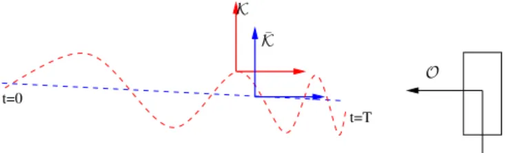
Let us define a virtual camera (Fig. 4) K that corresponds to the position of the on-board camera if there was no sway motion. The velocity of this virtual camera is ˙k, it is actually the velocity that is input into the reactive PG. Its value is given in(23). In order to compute a control law that does not include the sway motion, we will servo this virtual camera s(k) to s(k∗). t=0 t=T O ¯ K K
Fig. 4. K is the current camera frame and K is the camera position obtained if the visual servoing velocity is applied without the walking constraints.
We have now to express s = s(k) with regards to the current measurement s = s(k). With (14) we can write:
s(t) − s(0) = 8 t 0 5 L ˙kdt = 8 t 0 5 L( ˙k + ˙bk)dt (19) ands(t) − s(0) = 8 t 0 5 L ˙kdt (20)
Then assuming that s(0) − s(0) = E and using (19) and (20) we obtain s(t) = s(t) + 8 t 0 5 LkV c˙bdt − E (21)
from which we can deduce the corrected visual error
e(t) = s(t) − s∗ = e(t) − ( 8 t 0 5 LkV c˙bdt − E) (22)
Notice that whene −→ 0 then e −→30tL˙bk. In this study,
we do not expecte to converge to zero but to oscillate around zero with a period T . The convergence of the control law is then reached when 3t−Tt edt = 0, which is obtained if 3t t−T 3t 0L5 kV c˙bdt = 0. Let us define E = 3t t−T 3t 0L5 kV c˙bdt
and note that in generalE $= 0. It can be estimated over one period of time T . In order to avoid drift accumulation in the comutation of E we can use a sliding windows to define the current virtual error e and deduce the control law
˙k = −λ5L+ (e − ( 8 t 0 5 LkV c˙bdt − 8 t t−T 8 t 0 5 LkV c˙bdt)) (23)
And finally, the CoM reference velocity can be computed as : ˙c = −λcVkL5+(e − ( 8 t 0 5 LkVc˙bdt − 8 t t−T 8 t 0 5 LkVc˙bdt)) (24) D. Vision based control
Visual Model Predictive Control Scheme has been studied to deal with constraints, eg to ensure the visibility of the target or avoid joint limits [20]. In order to improve the results presented in this paper, we propose to write a general non linear model predictive control scheme to select the optimal jerk of the CoM ...C regarding some visual criteria. Then the function to minimise is now
min... C ,F 1 2 N 4 i=1 %s(ki) − s ∗ i% 2 (25) IV. APRELIMINARY RESULT
Fig. 5, Fig. 6 depicts an experiment of visual servoing for dynamic walking that shows the feasibility of the approach on the HRP2 robot.
The experimental scheme is the following : the robot has to reach a desired position with regards to a partially known object. First, the system is given a desired pose of the object in the camera frame. It can be arbitrarily set or it can be estimated by placing the robot at the desired position. The object is then tracked in the image and its pose is estimated
Fig. 5. Model tracking while walking on a square on the ground. The robot firstly walks forward, then sideways, then backwards, and sideways again to reach its initial position. On images 2-8, we can notice white horizontal curved line. They are induced by the reflexion of the light on the dark plastic shield. The model-tracker gives good positioning results when the tracked object has 3 dimensional edges.
in the camera frame. It allows to learn k∗
Mo. The advantage
of the learning solution is that the position is estimated using the same camera as the one used on-line for visual servoing, which compensate for calibration errors. Secondly the robot is placed to an initial arbitrary positionkMofrom where the
reference object can be seen. In this paper, the robot has to perform both translational motions and rotational motion to reach the desired position.
Fig. 5 presents some tracking results while the robot is walking. On images 2-8, we can notice white horizontal curved line. They are induced by the reflexivity of the light on the dark plastic shield that protects the HRP-2 camera. They cause some partial occlusion and worse, they can masquerade object lines and make the tracking fail. The model-based tracker we use is designed for convex objects. If the current projection of the model only allows to track 2D planes, it can happen that the optimisation problem falls in a local minimum. The order of magnitude of the model-tracking accuracy, while walking 2m away from the object, is about0.1m and 0.1rad.
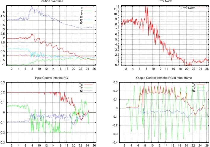
In the experiment illustrated Fig. 6 a position based visual servoing is given the Pattern Generator as an input. In this experiment, the robot has approximatly to move 1m forward, 1.5m sideways and 0.7rad in rotation. A convergence thresh-old is arbitrarily set to 0.1m in translation and 0.1rad in rotation. Then the accuracy of the positioning reaches these values at best. Besides, the reference velocity is limited to 0.2m/s in translation and 0.2rad/s in rotation. This limits have be chosen to secure the robot mechanical parts. It may be increase in the future.
The top left figure depicts the estimated position of the object frame with regards to the camera frame. Notice that the on board camera axis are not parallel to the ground plane. The robot head is oriented slightly towards the ground. Also remark that the position estimation could be replaced by any localisation technique (such as SLAM) except that the model based scheme has the advantage to handling mobile object tracking1. In the top left graph, we can see that the lateral
1
some examples of rolling ball tracking and other objects tracking are available on the lagadic team website : http://www.irisa.fr/lagadic/demo.html
motion oscillates. This is directly due to the stepping motion. This lateral motion can be also found in the bottom right figure that is the output velocity of the pattern generator. The walking control guaranties this sway motion to be minimal. Furthermore, the upper body of the HRP2 robot can not compensate for this sway motion due to a lack of degrees of freedom. Anyway, the model tracker proved to be robust enough to track an object even when the camera oscillates under the sway motion. The top right figure first shows an increase of the error and then a visual servoing classical exponential decrease. The increase of the error is directly related to the variation of the pose estimation that can be observed in the top left figure. Both changes are due to the motion induced by the robot first steps. Usually, the robot needs two steps to reach the desired velocity and make the error decrease. The bottom left figure presents the visual control law that is the reference pattern generator velocity.
The resulting motion has been compared to a planned trajectory executed with a Kajita’s PG. As shown in [21], when the robot is walking forward or backward, the open loop execution of the planned trajectory results in a good positioning (less than1cm in translation and less than 0.1rad in rotation). However, lateral motion induces a large drift and an error in rotation, such that the difference between the initial position and the final position is more than 60cm in translation and more that 0.5rad in rotation. Since we have set the convergence threshold to 0.1, the translational error is less than2cm. Yet, the error in rotation is small and less than 0.1rad even after lateral motion. The difference between the first position and the final position was less that 15cm and the error in rotation less than 0.1rad. As excepted, the greater error are found along the sagital plane. Indeed, this is the direction where the pose estimation is the more uncertain for a monocular camera.
V. CONCLUSION
We think that vision based control is well suited to control the walk of the humanoid robot HPR-2. The method proved to be robust to model errors and gives better result than executing a planned trajectory without closing the control loop. Our going work on vision based pattern generator
-1 -0.5 0 0.5 1 1.5 2 2.5 3 3.5 4 4.5 5 2 4 6 8 10 12 14 16 18 20 22 24 26
Position over time
x y z rx ry rz 0.5 1 1.5 2 2.5 3 3.5 4 4.5 5 5.5 6 6.5 7 7.5 8 8.5 9 9.5 10 10.5 11 11.5 12 2 4 6 8 10 12 14 16 18 20 22 24 26 Error Norm Error Norm -0.3 -0.2 -0.1 0 0.1 0.2 0.3 2 4 6 8 10 12 14 16 18 20 22 24 26
Input Control into the PG Tx Ty rz -0.4 -0.3 -0.2 -0.1 0 0.1 0.2 0.3 2 4 6 8 10 12 14 16 18 20 22 24 26
Output Control from the PG in robot frame Tx Ty Rz
Fig. 6. Visual servoing of dynamic walking experiment. Top left : trajectory of the object’s pose in the camera frame. Top right : evolution of the error norm. Bottom left : control Input of the pattern generator (reference CoM velocity ¯˙c). Bottom right : control output of the pattern generator (real CoM velocity ˙c), we can remark two picks to zero which are only due to client reading error from the middle ware and these values are not the one sent to the system
is expected to improve these results in several ways : the predictive framework allows to include both balance and visibility constraints, we expect the system to be more reactive and we expect more natural trajectories that do not necessary follows an exponential decrease of the error.
VI. ACKNOWLEDGMENTS
The first author is supported by Grant-in-Aid from the Japanese Society for the Promotion of Science (JSPS) Fel-lows P-09721. The second, third and fourth authors are supported by a grant from the RBLINK Project, Contrat ANR-08-JCJC-0075-01. Special thanks to F. Chaumette for his precious advices and discussions.
REFERENCES
[1] C. Kemp, A. Edsinger, and E. Torres-Jara, “Challenges for robot manipulation in human environments,” IEEE Robotics and Automation Magazine, pp. 20–29, march 2007.
[2] O. Lorch, A. Albert, J. Denk, M. Gerecke, R. Cupec, J. Seara, W. Gerth, and G. Schmidt, “Experiments in vision-guided biped walking,” in IEEE/RSJ International Conference on Intelligent Robots and Systems, 2002, pp. 2484–2490.
[3] J. Chestnutt, P. Michel, J. Kuffner, and T. Kanade, “Locomotion among dynamic obstacles for the honda asimo,” in IEEE Int. Conf. on Robotics and Automation, 2007, pp. 2572–2573.
[4] P. Michel, J. Chestnutt, S. Kagami, K. Nishiwaki, J. Kuffner, and T. Kanade, “Gpu-accelerated real-time 3d tracking for humanoid locomotion and stair climbing,” in IEEE Int. Conf. on Robotics and Automation, October 2007, pp. 463–469.
[5] J.-S. Gutmann, M. Fukuchi, and M. Fujita, “3d perception and envi-ronment map generation for humanoid robot navigation,” International Journal of Robotics Research, vol. 27, no. 10, pp. 1117–1134, 2008. [6] J. Coelho, J. Piater, and R. Grupen, “Developing haptic and visual perceptual categories for reaching and grasping with a humanoid robot,” Robotics and Autonomous Systems, vol. 37, no. 2-3, pp. 195– 217, November 2001.
[7] G. Taylor and L. Kleeman, “Flexible self-calibrated visual servoing for a humanoid robot,” in Australian Conference on Robotics and Automation (ACRA2001), 2001, pp. 79–84.
[8] N. Courty, E. Marchand, and B. Arnaldi, “Through-the-eyes control of a virtual humano¨ıd,” in IEEE Computer Animation 2001, H.-S. Ko, Ed., Seoul, Korea, November 2001, pp. 74–83.
[9] N. Mansard, O. Stasse, F. Chaumette, and K. Yokoi, “Visually-guided grasping while walking on a humanoid robot,” in IEEE Int. Conf. on Robotics and Automation, ICRA’07, Roma, Italy, April 2007, pp. 3041–3047.
[10] M. Morisawa, K. Harada, S. Kajita, S. Nakaoka, K. Fujiwara, F. Kane-hiro, K. Kaneko, and H. Hirukawa, “Experimentation of humanoid walking allowing immediate modification of foot place based on analytical solution,” in IEEE Int. Conf. on Robotics and Automation, 2007, pp. 3989–3994.
[11] K. Nishiwaki and S. Kagami, “Online walking control system for hu-manoids with short cycle pattern generation,” Int. Journal of Robotics Research, vol. 28, pp. 729–742, 2009.
[12] A. Herdt, D. Holger, P. Wieber, D. Dimitrov, K. Mombaur, and D. Moritz, “Online walking motion generation with automatic foot step placement,” Advanced Robotics, vol. 24, no. 5-6, pp. 719–737, April 2010.
[13] A. Herdt, N. Perrin, and P.-B. Wieber, “Walking without thinking about it,” in IEEE Int. Conf. on Robotics and Automation.
[14] C. Dune, A. Herdt, O. Stasse, P.-B. Wieber, E. Yoshida, and K. Yokoi, “Cancelling the sway motion of dynamic walking in visual servoing,” in IEEE Int. Conf. on Robotics and Automation, 2010.
[15] N. Perrin, S. Stasse, F. Lamiraux, and E. Yoshida, “Approximation of feasibility tests for reactive walk on hrp-2,” in IEEE International Conference on Robotics and Automation (ICRA), 2010, pp. 4243– 4248.
[16] P.-B. Wieber, “On the stability of walking systems,” in Int. Workshop on Humanoid and Human Friendly Robotics, 2002.
[17] A. Comport, E. Marchand, M. Pressigout, and F. Chaumette, “Real-time markerless tracking for augmented reality: the virtual visual servoing framework,” IEEE Trans. on Visualization and Computer Graphics, vol. 12, no. 4, pp. 615–628, July 2006.
[18] Huber, Robust Statistics. Wiler New York, 1981.
[19] F. Chaumette and S. Hutchinson, “Visual servo control, part i: Basic approaches,” IEEE Robotics and Automation Magazine, vol. 13, no. 4, pp. 82–90, December 2006.
[20] G. Allibert, E. Courtial, and F. Chaumette, Visual Servoing via Advanced Numerical Methods. Springer, Avril 2010, ch. 20- Visual Servoing via Nonlinear Predictive Control, pp. 393–412.
[21] O. Stasse, A. Davison, R. Sellouati, and K. Yokoi, “Real-time 3d slam for humanoid robot considering pattern generator information,” in IEEE Int. Conf. on Robotics and Automation, 2006, pp. 348–355.