HAL Id: hal-01941676
https://hal.archives-ouvertes.fr/hal-01941676
Submitted on 1 Dec 2018HAL is a multi-disciplinary open access archive for the deposit and dissemination of sci-entific research documents, whether they are pub-lished or not. The documents may come from
L’archive ouverte pluridisciplinaire HAL, est destinée au dépôt et à la diffusion de documents scientifiques de niveau recherche, publiés ou non, émanant des établissements d’enseignement et de
A distributed multi-agent production planning and
scheduling framework for mobile robots
Stefano Giordani, Marin Lujak, Francesco Martinelli
To cite this version:
Stefano Giordani, Marin Lujak, Francesco Martinelli. A distributed multi-agent production planning and scheduling framework for mobile robots. Computers & Industrial Engineering, Elsevier, 2013, 64 (1), pp.19-30. �hal-01941676�
A Distributed Multi-Agent Production Planning and
Scheduling Framework for Mobile Robots
Stefano Giordani ∗ Marin Lujak † Francesco Martinelli ‡
Abstract
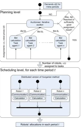
Inspired by the new achievements in mobile robotics having as a result mobile robots able to execute different production tasks, we consider a factory producing a set of distinct products via or with the additional help of mobile robots. This particu-larly flexible layout requires the definition and the solution of a complex planning and scheduling problem. In order to minimize production costs, dynamic determination of the number of robots on each production task and the individual robot allocation are needed. We propose a solution in terms of a two-level decentralized multi-agent sys-tem (MAS) framework: at the first, production planning level, agents are tasks which compete for robots (resources at this level); at the second, scheduling level, agents are robots which reallocate themselves among different tasks to satisfy the requests coming from the first level. An iterative auction based negotiation protocol is used at the first level while the second level solves a Multi-Robot Task Allocation Problem (MRTA) through a distributed version of the Hungarian Method. A comparison of the results with a centralized approach is presented.
Keywords: Production scheduling; Multi-robot task allocation; Multi-agent system; Optimization algorithm; Computer simulation.
∗Corresponding author. Dipartimento di Ingegneria dell’Impresa, Universit`a di Roma “Tor Vergata”,
Via del Politecnico, 1 - 00133 Roma, Italy. e-mail: [email protected]
†University Rey Juan Carlos, CETINIA, Calle Tulipan s/n, 28933 Mstoles (Madrid), Spain. e-mail:
‡Dipartimento di Informatica, Sistemi e Produzione, Universit`a di Roma “Tor Vergata”, Via del
1
Introduction
An external demand of a manufacturing system is generally a fluctuating stochastic pro-cess, usually known with a satisfactory accuracy only over a limited time horizon ahead. This introduces, at the strategic level, a high degree of uncertainty in the design of a production system and a supply chain where critical decisions must be taken based on aggregate and approximate information (see, e.g., Mun, 2002).
In traditional shop-floor planning, establishing a production facility requires the selec-tion of static producselec-tion machines and robot manipulators which would be suitable for long term production plans. With the advances in the development of mobile production resources, now it is possible for many products, once manufactured only by large pro-duction machines permanently tied to single locations, to be manufactured with smaller, mobile robots. One of the first such robots was presented in July 2010 by robotic producer Kuka (Bischoff et al., 2010). The shop floor layout with mobile robots makes the strategic decisions less critical with respect to the ones associated to the design of a plant where machines (i.e., production resources) are located on static positions. A dynamic layout represents in fact a less constrained facility where design decisions are postponed to the operative level and become reversible options. A dynamic layout is more effective in re-sponding to a fluctuating external demand and can be considered, for this reason, in the same vein as other solutions adopted through the years in the manufacturing domain for the same purpose, like, among others, Flexible Manufacturing Systems (e.g., Huang and Chen, 1986), Group Technology (see, e.g., Selim et al., 1998), Holonic Manufacturing (see, e.g., Christensen, 1994), and Agile Production Systems (see, e.g., Dugnay et al., 1997).
The high degree of flexibility achieved by the proposed dynamic multi-robot layout leads to a more complex operation management which may render centralized architec-tures unviable. Centralized architecarchitec-tures in such complex environments are often imprac-tical because of computational and communication bottleneck and the vulnerability of system failure. On the other hand, a bottom-up multi-agent modular architecture dis-tributes computational resources and capabilities among the agents and does not suffer from the “critical point of failure” problem associated with centralized systems (see, e.g., Wooldridge, 2002). Further advantages of a decentralized multi-agent approach are mod-ularity, decentralized knowledge bases, fault-tolerance, redundancy and extendibility, in
the sense that new robots can be added to the original system without any change in the system architecture (see, e.g., Lueth and Laengle, 1994).
For all the above reasons and because mobile robots are autonomous entities with limited vision and communication capacities, in this paper we propose a decentralized two-level multi-agent system (MAS) framework for the case where the production is exe-cuted exclusively or with the additional help of mobile robots, as shown, e.g., by Helms et al. (2002) and Tan et al. (2009). On the first, production planning level, tasks compete for the resources (robots) required for their execution. Assuming that the planning time horizon is subdivided into a finite number of time periods, the objective of the production planning level is the determination of the assignment of the robots in each time period to the respective tasks in order to minimize the total production cost for each produc-tion process (with the products’ demand known over all the time periods in the given time horizon). The resulting problem is a multiple decision maker multi-item dynamic lot-sizing problem with limited production capacity. The problem is NP-hard since it can be shown to generalize the very special case with single-decision maker, single-item, zero inventory holding cost, convex pro-duction cost function, unit set-up cost, and no propro-duction capacity, that has been proved to be NP-hard by Florian et al. (1980). Since the problem at production planning level is NP-hard this level of the MAS framework is coupled with a heuristic iterative auction based negotiation protocol to coordinate the agents’ decisions (see, e.g.: Kutanoglu and Wu, 2006; Schneider et al., 2005; Roundy et al., 1991). The resource prices, needed for the iterative auction based protocol, are updated using a strategy inspired by the subgradient technique used in the Lagrangian relaxation approach (see, e.g., Chen et al., 1998, and Barahona and Anbil, 2000).
Given the number of robots assigned to the tasks in each time period according to the decisions made at the first, planning level, on the second, scheduling level, the objective is to minimize the total distance covered by the robots in the reallocation between consec-utive periods. Therefore, a Multi-Robot Task Allocation Problem (MRTA) is solved for each period. The objective of the MRTA problem is to find the assignment of n robots to a set of n tasks (target positions) based on the optimization of some global objective function (see, e.g., Gerkey and Mataric, 2003). We assume that the decision making
en-vironment for this level is decentralized as well, with as many decision makers (agents) as there are the robots in the system. In particular, we assume robot to be collaborative, homogeneous, arranged in regular networks and relying on local communication between neighboring agents. We use a distributed version of the Hungarian Method for this alloca-tion problem, a distributed combinatorial optimizaalloca-tion algorithm which solves the assignment problem in strongly polynomial time (Giordani et al., 2010).
Note that the problem definition and the proposed modeling framework are general enough so that the task scheduling problem and the solution model can be applied also to other types of mobile manufacturing resources and production operators.
We experiment the proposed model considering a fluctuating demand modeled through an ARMA process. To measure the effectiveness of the approach, the social welfare (see, e.g., Chevaleyre et al., 2006) of the task agents in the decentralized scenario is compared with the performance obtained through a centralized solution. Preliminary results re-garding the first level of the proposed framework have been presented by Giordani et al. (2009) where the problem addressed on the second level (the robot movement) was not considered. The integrated solution of the two levels is a viable solution for the incorpo-ration of mobile robots on the shop-floor and provides indeed an interesting insight into the problem. In particular, we show that the decentralized approach of the first level gives comparable results to the centralized one while the required total movement distance of the robots’ reallocation is in general inferior.
The remainder of the paper is organized as follows. We introduce related work and review some of the economic models used in MAS negotiation for resource allocation in Section 2. In Section 3, the decentralized production scheduling problem is presented. The two-level solution approach is given in Section 4. In Section 5, we present the simulation results. We close the paper with the conclusions in Section 6.
2
Related work
There is a vast literature on the scheduling techniques in manufacturing based on multi-agent systems (see, e.g., Shen et al., 2006, Shen et al., 2007, Wang et al., 2008). For multi-agent interaction and negotiation, there are several applicable
economic models which might work well for the production planning level of the presented framework where tasks compete for resources (robots): commodity market, posted price, bargaining, tender/contract-net, and auction model (see, e.g., Kraus, 2001, Chevaleyre et al., 2006, Buyya et al., 2002), which is the approach chosen in this paper.
Regarding the second level, MRTA corresponds to the (linear sum) Assignment prob-lem for which the first developed algorithm was the Hungarian method (Kuhn, 1955). The Hungarian method or Kuhn-Munkres algorithm is a well known iterative algorithm which maintains dual feasibility during calculation and searches for a primal solution satisfying complementary slackness conditions. If the primal solution is feasible, the solution is optimal. If the primal solution is not fea-sible, the method performs a modification of the dual feasible solution after which a new iteration starts. Hungarian method can be implemented using
the alternating trees so that its worst case time complexity is limited by O(n3
) (see, e.g., Papadimitriou and Steiglitz, 1982).
There are several main approaches to the Assignment problem (see, e.g., Burkard and C¸ ela, 1999). The classical centralized assignment methods find a solution through the iterative improvement of some cost function: in primal simplex methods it is a primal cost, and in Hungarian, dual simplex and relaxation methods it is a dual cost (see, e.g., Bertsekas, 1992).
The Auction algorithms can improve as well as worsen both the primal and the dual cost through the intermediate iterations, although at the end, the optimal assignment is found (Bertsekas, 1992). Bertsekas in this work introduces the auction algorithm in which the agents bid for the tasks in iterative manner, and in each iteration, the bidding increment is always at least equal to ǫ (ǫ-complementary slackness). If ǫ < 1
n the algorithm
finds the optimal solution, and it runs in O(n3·max{c
ij}) time, where cij is the assignment
cost of robot i to task j, that is in pseudo-polynomial time. Using ǫ-scaling
technique and appropriate data structures a polynomial time version of the
auction algorithm running in O(n3
log(n · max{cij}) time is given by Bertsekas
and Castanon (1989) and Bertsekas (1992).
Zavlanos et al. (2008) provide a distributed version of the auction algorithm proposed by Bertsekas for the networked systems with the lack of global information due to the
limited communication capabilities of the agents. Updated prices, necessary for accurate bidding can be obtained in a multi-hop fashion only by local exchange of information between adjacent agents. No shared memory is available and the agents are required to store locally all the pricing information. This approach calculates the optimal solution in O(∆ · n3· max{c
ij}) time, with ∆ ≤ n − 1 being the maximum network diameter of the
communication network.
There are also many parallel algorithms based on the Hungarian method. For a good
survey see, e.g., Burkard and C¸ ela (1999), and Bertsekas et al. (1995). Among other
parallel algorithms for the assignment problem, one of the most efficient is the one proposed by Orlin and Stein (1993) that adopting cost scaling technique
solves the problem using Ω(n4
) processors in O(log3n · log C) time.
In the robotic community, there are many heuristic methods developed for the MRTA problem. Smith and Bullo (2007) describe two algorithms, namely ETSP, and Grid algo-rithm, for the task assignment in the sparse and dense environments. The agents have a full knowledge of the tasks in the environment and, in the ETSP algorithm, approach the closest ones. If the closest task is occupied, they pre-compute an optimal tour through the n remaining tasks, and search for the first non-occupied task based on certain crite-ria. Gerkey and Mataric (2003, 2004) describe certain relevant heuristic algorithms for the MRTA problem through the prism of three important factors: computation and communi-cation requirements, and the manner in which tasks are considered for (re)assignment, i.e. whether all or just a part of the tasks are considered for (re)assignment in each iteration. The problem with these approaches, as the authors state, is that there is no characteriza-tion of the solucharacteriza-tion quality that can be expected by the algorithms. Kwok et al. (2002) apply the classic combinatorial methods, such as Hungarian and Gabow algorithms, to the assignment problem in the context of a set of mobile robots which need to be moved to a desired matrix of grid points to have a complete surveillance of the desired area.
3
Problem formulation
A manufacturing system producing P different types of goods is considered. A task denotes a production process of a particular type of product and all the tasks are assumed different from one another. The tasks are executed by a set of N identical mobile robots,
characterized by a hiring cost, defined below.
Given a finite time horizon of T time periods and assuming that the demand for the P products in the T time periods is known, the discrete time production scheduling problem addressed in this paper consists of finding how many robots must be assigned to each task in each time period in order to minimize a total cost composed of backlog, inventory, manufacturing, and robot hiring costs.
Once the solution to the task scheduling problem has been determined, the robots decide how to move in order to fulfill the assignment requests by covering the minimum total distance.
A two-level hierarchical decentralized production scheduling problem can be then for-mulated, where, at the first level, the tasks are considered as agents which compete for robots, resources characterized by a hiring price; at the second level, robots are the agents which autonomously decide upon the way to meet the requests of the first level.
3.1 Production planning level
At the first, production planning level, each task agent requests the task coordinator agent for robots for each time period, based on product demands and production costs. The task coordinator agent assigns the robots to the tasks for each unit time period on the basis of their requests.
For all time periods k = 1, . . . , T , the agent representing task i, related to product
i, knows product demand rate di(k), robot maximum production rate ri(k) (production
capacity), unitary manufacturing cost ci(k), unitary holding cost hi(k), unitary backlog
cost bi(k), and unitary robot hiring cost ρi(k), all nonnegative. It is reasonable to assume
that the robots’ displacement time is negligible in respect to the length of the time period, ∆t. For each time period k, the decision variables controlled by the agent representing task i are:
• ni(k) ≥ 0: required number of robots (robot request);
• ui(k) ≥ 0: production rate.
Production can be anticipated or delayed in respect to the product demands, resulting in holding and backlog costs, respectively. Each task i is associated with a buffer whose
content xi(k) at the end of time period k can be positive (if a stock of completed product
items is present in the buffer) or negative (if a backlog of demands for the product realized with task i is in the queue). Using a standard notation, we denote x+i (k) := max{xi(k), 0}
as the stock level, and x−i (k) := max{−xi(k), 0} as the backlog level at the end of time
period k. Notice that, for each time period k, and task (product) i, only one of x+i (k) and x−i (k) can be different from 0 (i.e., x+i (k) · x−i (k) = 0 for k = 1, . . . , T and i = 1, . . . , P ).
The local optimization problem addressed by every task agent i includes x+i (k) and x−i (k) as additional variables, for each time period k. Those variables, together with the production rates ui(k), are assumed to be continuous according to a fluid approximation.
Given the above parameters and variables, the local optimization problem, Pi, addressed
by each task agent i can be formulated as follows.
(Pi) : min zi= T X k=1 h hi(k)x + i (k) + bi(k)x−i (k) + ci(k)ui(k) + ρi(k)ni(k) i (1) s.t. x+i (k) − x−i (k) = x+i (k − 1) − x−i (k − 1) + ∆t[ui(k) − di(k)], k = 1, ..., T (2) ui(k) ≤ ri(k) ni(k), k = 1, ..., T ; (3) ui(k), x+i (k), x − i (k), ≥ 0, k = 1, ..., T ; (4) 0 ≤ ni(k) ≤ N and integer, k = 1, ..., T. (5)
The values of x+i (0), x−i (0), and ni(0) represent the initial conditions, i.e. the stock
level, the backlog level, and the number of preassigned robots to task i respectively, at the beginning of the planning time horizon. For simplicity, but w.l.o.g., these values are assumed to be equal to zero. Constraints (2) are the mass balance constraints among product demand ∆t · di(k), stock level x+i (k), backlog level x
−
i (k), and production level
∆t · ui(k), for each time period k. W.l.o.g., assuming that, for each time period k and for
each task i, the values of hi(k) and bi(k) are positive, the constraint x+i (k) · x −
i (k) = 0,
is implicitly satisfied by the optimal solution, and, hence, omitted in the formulation.
capacity ri(k) · ni(k). Problem (Pi) belongs to the class of deterministic dynamic
lot-sizing problems well known in the inventory management literature (see, e.g., Florian et al., 1980).
For each task agent i, let n∗
i(k) be the number of required robots at time period k, in
the optimal solution of problem Pi, and let zi∗ be the optimal solution of Pi. Each task
agent (decision maker) finds such a solution taking into account only its local objective and constraints, but shares with the other task agents limited amount of available robots (resources). Therefore, these local decisions can be implemented only if the following global constraints are satisfied.
P
X
i=1
n∗i(k) ≤ N, k = 1, ..., T. (6)
In general, this is not the case and, hence, a negotiation process must be implemented among the task agents to come up with a set of local solutions that together satisfy also constraints (6). We assume that this process is supervised by another decision maker, i.e., a coordinator agent, which can be an arbitrary preassigned task agent that assigns the robots to the tasks for each time period on the basis of their requests, guaranteeing the fulfillment of the constraint on the limited robot amount. In Section 4.2, we provide a model for such a negotiation.
3.2 Production scheduling level
On the second, production scheduling level, which represents robots’ allocation to task locations, the scope is to assign individual robots to tasks so as to minimize total movement cost (i.e., total distance traveled by robots among task locations) during the planning time horizon, given the number ni(k) of robots required by task i (with i = 1, . . . , P ) in period
k (with k = 1, . . . , T ) according to the decisions made at the first level.
Let ℓi be the location where task i is executed. We assume that at the beginning of
the planning time horizon the robots are located at a depot whose location is ℓ0, and that
at the end of the planning time horizon, all the used robots must leave the task locations and go back to the depot. Let d(ℓi, ℓj) be the distance that a robot has to travel to go
from location ℓi to location ℓj, with i, j = 0, 1, . . . , P . The distances among locations are
that the depot is located at an equidistant point from the task locations.
Therefore, at the beginning of the first time period, ni(1) robots leave the depot and
move to location ℓiof task i, for each task i = 1, . . . , P . Successively, for each k = 2, . . . , T ,
at the beginning of period k, the robots should be reallocated among the task locations with possibly some additional robots leaving the depot and going to the required task locations, such that at the beginning of period k (at least) ni(k) robots are located at
location ℓi of task i.
Let N (k) ≤ N be the maximum number of robots used during the first k periods, i.e., N (k) = maxh=1,...,k{PPi=1ni(h)}, with k = 1, . . . , T , and let N (0) = 0. Since the locations’
distances satisfy the triangle inequality, we may assume that only if N (k) > N (k − 1), we have that N (k) − N (k − 1) additional robots leave the depot and reach some target (task) locations exactly at the beginning of period k. On the contrary, if N (k) = N (k − 1)
and PP
i=1ni(k) < N (k − 1), (at least) N (k) −PPi=1ni(k) robots will remain at their
current (task) locations also during period k, assuming that at each task location there is sufficient room to park also unused robots. Therefore, let us denote with n′i(k) ≥ ni(k)
the number of robots located at location ℓi during period k, where n′i(k) − ni(k) is the
number of robots parked at that location but not used by task i during period k. Clearly
PP
i=1n′i(k) = N (k). Finally, we may therefore assume that only at the end of the planning
time horizon the robots return to the depot.
According to the above considerations, in order to minimize the total distance traveled by the robots during the planning time horizon, we can independently minimize the total distance traveled by the robots for their reallocation to task locations between each two consecutive time periods k − 1 and k, with k = 2, . . . , T ; let us denote with D(k) the minimum total distance covered by the robots during reallocation k. The minimum total
distance traveled by the robots is D = PT +1
k=1 D(k), where D(1) is the total distance
traveled by ni(1) robots from the depot location ℓ0 to the task location ℓi, for each task
i, at the beginning of time period 1, and D(T + 1) is the total distance traveled by the robots to go back to the depot location from their last locations at the end of the planning time horizon. Clearly, D(1) does not depend on the (successive) robot reallocations. The same applies also to D(T + 1), since it is assumed that ℓ0 is located at equidistant position
Let us therefore consider the robots’ reallocation problem between two consecutive periods k − 1 and k, with k = 2, . . . , T . We model this problem considering a set R of N (k) collaborative mobile robots, a set T of N (k) targets (tasks), and a given N (k)×N (k) matrix of costs γrt for allocating robot r to target t. The problem faced by the robots is
determining the allocation of robots to targets such that each robot is allocated exactly to one target, each target is allocated to exactly one robot, and the total allocation cost is minimized.
The cost γrt for allocating robot r to target t depends on the (current) location of
robot r and the location of target t.
Since the robots are assumed to be of the same type, without loss of generality, we can
re-index them such that robot r ∈ {1 +Pi−1
h=1n′h(k − 1), . . . ,
Pi
h=1n′h(k − 1)}, is assumed
to be located at location ℓi of task i (with i = 1, . . . , P ), and robot r ∈ {1 +PPh=1n′h(k −
1), . . . , N (k)}, is a (new) robot that starts to be used for the first time in period k and therefore is assumed to be located at the depot location ℓ0, and has to go to a certain
task location at the beginning of period k. Similarly, the targets are indexed so that target t ∈ {1 +Pi−1
h=1nh(k), . . . ,Pih=1nh(k)}, is located at location ℓi, with i = 1, . . . , P ,
and target t ∈ {1 +PP
h=1nh(k), . . . , N (k)}, is a dummy (fictitious) target assumed to be
located at the dummy (fictitious) location ¯ℓ. Finally, cost γrt is assumed as the distance
between the location of robot r and the location of target t if the latter is non-dummy, otherwise such cost is assumed to be equal to zero since allocating a robot to the dummy target means that this robot will be unused in period k and hence it will remain parked at its previous location during that period.
The mathematical formulation of the problem is
minX r∈R X t∈T γrt· xrt (7) s.t. X r∈R xrt= 1, ∀ t ∈ T , (8) X t∈T xrt= 1, ∀ r ∈ R, (9) xrt≥ 0, ∀ r ∈ R, ∀ t ∈ T , (10)
and it corresponds to the well known Assignment problem. Although fractional solutions may exist, there always exists an optimal integer solution which corresponds to a real
assignment, since no fractional solution is a basic feasible solution of the above linear program (see, e.g., Papadimitriou and Steiglitz, 1982). In particular, xrt = 1 if the robot
r is assigned to target t; otherwise xrt= 0.
Denoting the above problem formulation as the primal problem, it is possible to define the dual problem as follows. Let αt be the dual variable related to target t, and βr the
same related to robot r. Both dual variables are real and unrestricted in sign. The dual problem is max{X r∈R βr− X t∈T αt} (11) s.t. βr− αt≤ γrt, ∀ r ∈ R, ∀ t ∈ T . (12)
It is possible to give an economic interpretation to the dual problem and the dual variables: αt is the price that each robot r will pay if it gets assigned to target t, while βr is the
robot r’s utility for being assigned to a certain target. Constraint (12) of the dual problem states that the utility βr of robot r cannot be greater than the total cost (γrt+αt) faced by
robot r for being assigned to target t. The dual objective function (11) to be maximized is the difference between the sum of the utilities of the robots and the sum of the prices of the targets, i.e., the total net profit of the robots. On the basis of the duality in linear
programming,P
rβr−Ptαt≤Pr
P
tγrt· xrt; therefore, the total net profit of the robots
cannot be greater than the total assignment (displacement) cost that the robots have to pay for being assigned to the targets, and only at the optimum, those two are equal. Obviously, at the optimum, each robot r will be assigned to target t for which the utility of the robot is βr = γrt+ αt, i.e., exactly equal to the total cost that the robot r would
pay for being assigned to target t.
4
Solution approach
The problems associated with the production planning and scheduling level are solved by two different and decentralized algorithms, the first one consisting of a negotiation among the tasks, and the second one amounting to a distributed version of the Hungarian algorithm, executed collaboratively by the robots.
4.1 Two-level MAS planning and scheduling framework
The two-level multi-agent system framework for planning and scheduling of production with mobile robots is shown in Figure 1.
[Insert Figure 1 around here]
At the first, planning level, the negotiation among the tasks is modeled by an iterative auction process controlled by the coordinator agent which is in charge of coordination of the negotiation. The details regarding the auction process are found in Section 4.2. Once when, at the planning level, the number of robots assigned to each task for each time period k ∈ {1 . . . T } is known, the planning level ends and the scheduling level begins its performance with the aim to find for each robot exact movements on the shop-floor through the whole time horizon subdivided in T time periods.
4.2 First level: negotiation process among the tasks
In the iterative auction process among tasks, at each iteration:
Step 1 The coordinator (auctioneer) communicates to all the task agents (bidders) current prices of the robots in the T time periods;
Step 2 Each task agent, based on the local utility function of its local objective, the constraints, and the current robot prices, determines the robot requests (a bid) for the T time periods maximizing its utility function and communicates its robot requests to the coordinator;
Step 3 Based on the bids received from the task agents, the coordinator allocates the robots to the tasks for each time period, maximizing the robots’ total utility func-tion;
Step 4 In order to reduce possible conflicts among tasks generated by their bids (i.e., the violation of constraints (6)), or to stimulate usage of the robots, the coordinator updates the robot prices.
Iteration process repeats until a certain (halting) condition is reached (e.g., a maximum number of iterations have been performed, or the best robot allocation found is sufficiently good from the agents’ point of view). At the end, the best robot allocation is retrieved.
Let Bi = {ni(k) : k = 1, . . . , T } be the bid of task agent i, and let Λ = {λ(k) : k =
1, . . . , T } be the (current) set of the robot prices fixed by the coordinator (each one for each time period). The utility function Ui(Bi, Λ) of agent i is the opposite of the total
production cost during the planning time horizon:
Ui(Bi, Λ) = −zi∗(Bi) − p(Bi, Λ). (13)
In this expression, z∗
i(Bi) is the (minimum) production cost for task i with fixed
num-bers of assigned robots ni(k), with k = 1, . . . , T , according to bid Bi, and p(Bi, Λ) =
PT
k=1λ(k)ni(k) is the (additional) robot cost. Note that, zi∗(Bi) is the optimal solution
of the local optimization problem Pi with fixed values of ni(k).
In Step 2, agent i finds the best bid B∗
i = {n∗i(k) : k = 1, . . . , T }, i.e., the bid that
maximizes its utility function Ui(Bi, Λ). Let Ui∗(Λ) be its maximum value for a given
set Λ of robot prices. Finding B∗
i, and hence determining Ui∗(Λ), corresponds to solving
problem Pi with λ(k) added to the robot hiring cost ρi(k) in the objective function of Pi.
In Step 3, the coordinator receives bid B∗
i from each task i, and assigns robots to
tasks maximizing resources’ (robots’) utility function taking into account received bids.
Denoting with νi(k) the number of robots assigned to task i in time period k, robots’
utility function R(ν, Λ) is the total profit obtained from the robot assignment, and, hence, R(ν, Λ) = T X k=1 λ(k) P X i=1 νi(k). (14)
Since νi(k) cannot be greater than robot request (bid) n∗i(k) of task agent i and
PP
i=1νi(k)
cannot be greater than N , for each k = 1, ..., T , the maximization of R(ν, Λ) can be easily obtained by (heuristically) assigning robots to tasks on the basis of the values of n∗
i(k),
for example adopting one of the following rules and taking the best related solution. • Rule 1. For each time period k, order the tasks according to non-increasing robot
requests n∗i(k), and, following this task order, assign νi(k) = min{n∗i(k), N′(k)}
robots to task i, where N′(k) (with 0 ≤ N′(k) ≤ N ) is the number of non-assigned
(yet available) robots in time period k.
• Rule 2. For each time period k, assign proportionally robots to tasks according to the robot requests n∗
i(k), that is, denoting with w(k) = min{1, (N/
P
assign νi(k) = w(k) · n∗i(k) (approximating the value to the closest integer) robots
to task i in time period k, and such that P
iνi(k) ≤ N .
Quality of robot assignment is evaluated from the task agents’ point of view, measuring the social welfare w(ν) of the tasks related to a given robot assignment ν = {νi(k)|i =
1, . . . , P, k = 1, . . . , T } as the (minimum) total production cost of the tasks with that robot assignment, that is,
w(ν) = P X i=1 zi∗(νi), (15) where z∗
i(νi) is the optimal solution of Pi with a given number of robots ni(k) = νi(k)
assigned to task i, for each time period k. Let w∗be the best (minimum) value of the social welfare found so far during iterative auction process. It can be proved that expression
wL(Λ) = − P X i=1 Ui∗(Λ) − N T X k=1 λ(k), (16)
is a valid lower bound on the best value of the task agents’ social welfare, for any vector Λ of non-negative robot prices λ(k).
In Step 4, the coordinator updates the robot prices λ(k), with k = 1, ..., T . This is done, considering the deviation dev(k) =PP
i=1n∗i(k) − N of the total number of requested
robots from the number N of available robots, and by increasing the current value of λ(k) if dev(k) is positive (i.e., dev(k) is the excess of robot requirements), or decreasing it (at most to 0) if dev(k) is negative (in this latter case −dev(k) is the deficit of robot requirements). The value of the increase (decrease) of λ(k) should be a non-decreasing function of the excess (deficit); moreover, it is a good practice that the auctioneer is more aggressive in the early iterations to get very quickly a good robot assignment, while smaller adjustments can be made in later iterations to refine the quality of the same. A possible choice for the price updating that goes in this direction is that of using an algorithm inspired by the subgradient technique used in Lagrangean relaxation, that experimentally guarantees the convergence of the Lagrangean dual (see, e.g., Held et al., 1974).
At iteration h of the auction process, let devh(k) be the deviation of the robot
require-ments, and Λh be the vector of the robot prices λh(k), with k = 1, . . . , T . The new value
of the robot price in time period k at iteration h + 1 is: λh+1(k) = max ( 0, λh(k) + ψh w ∗− w L(Λh) PT k=1(devh(k))2 devh(k) ) , (17)
where ψh is a scalar controlling the aggressiveness of the auctioneer. Following analog
practice in Lagrangean relaxation (see, e.g., Held et al., 1974) we start with value ψ0
= 2, and halve its value if the best task social welfare value found so far is not improved within a certain number of iterations.
In Step 1, the amount of information going from the coordinator to task agents is O(P · T · log(λmax)) bits, where λmax is the maximum robot price. In Step 2, the amount
of information sent by task agents to the robot owner is O(P · T · log(N )) bits. Step 3 is done in O((P log P ) · T ) time. Finally, in Step 4, price update is done in O(P · T ) time.
4.3 Distributed robot allocation algorithm
This section provides a distributed robot allocation algorithm for the problem of robots’ reallocation among task locations, i.e., targets, between two consecutive periods k − 1 and k of the planning time horizon. As discussed above, this corresponds to the well known Assignment problem where n robots have to be assigned to n targets, with n = N (k).
It is assumed that each robot r has the information of the distances (assignment costs) between its current location and the locations of all the targets. The inter-robot communication is performed over a connected dynamic communication network and the solution to the assignment problem is reached without any common coordinator or a shared memory of the system.
To solve the problem in this context, we developed a distributed version of a Hungarian method for the assignment problem, based on the concept of augmenting paths from the graph theory that we recall briefly in the following.
We refer to the centralized version of the Hungarian method implemented by means of so-called alternating trees and running in O(n3
) time (see, e.g., Burkard and C¸ ela, 1999). The algorithm is iterative and, maintaining a feasible dual solution, considers the admissible bipartite graph ¯G = (RST , ¯
E) where ¯E = {(r, t) : γrt+ αt− βr = 0}. The
algorithm searches for a matching of maximum cardinality in the graph ¯G. If the matching is perfect, i.e., if every robot is matched with a target, then the matching represents an optimal solution of the robot allocation and the algorithm stops. If the matching is not perfect, the algorithm updates the dual variables so as to increase the dual objective function such that at least one new admissible edge is added to ¯G, and continues with a
new iteration.
Given ¯G, let M ⊆ ¯E be the current maximal matching in ¯G. The edges belonging
to M are called matched edges, and the ones in ¯E\M are free edges. Given ¯G and the
current maximal matching M ⊆ ¯E, the algorithm iteratively improves the matching along
augmenting paths over alternating trees in ¯G, rooted at free target vertices. An alternating tree is a subgraph of ¯G with each target vertex connected to all its adjacent robot vertices through free edges of ¯E, and with each robot vertex connected to a target vertex through a matched edge. When an alternating tree rooted at free target vertex reaches a target leaf vertex which is adjacent to some free robot vertex, an augmenting path is found, i.e., a path that lets the augmentation of the cardinality of the matching, by exchanging the free and matched edges. When all the possible augmentation steps are performed, and hence
the resulting matching in ¯G is of maximum cardinality, the dual variables are updated
and the new admissible edges are added. Then a new iteration begins searching for the maximum matching on the new admissible graph (see, e.g., Burkard and C¸ ela, 1999).
In our distributed implementation of the Hungarian method, we maintain the forest F1
of all the alternating trees rooted at free target vertices. Moreover, we maintain the forest F2 of the alternating trees in ¯G rooted at robot vertices containing all the robot/target
vertices not contained in F1
. Clearly, the alternating trees in F2
are not connected with vertices in F1.
Initially, all the vertices of ¯G are assumed isolated (i.e., ¯E = ∅), and hence forests F1
and F2
are set up in the following way. Forest F1
is composed of n isolated target vertices. Forest F2
, in the similar way, is made of n isolated robot vertices. Dual variables are initially assumed to be αt= 0, for all the targets t, and βr= mint{γrt}, for all the robots r,
and are updated as follows. For each robot vertex r ∈ F2
, let σr= mint∈F1{γrt+ αt− βr}
be the minimum slack value of the dual constraints (12) associated to robot r among target vertices t in F1
, and let tr be the target corresponding to the arg-min; moreover,
let δ = minr∈F2{σr} be the minimum value among the minimum slack values of the robot
vertices r in F2
. The new (feasible) values of the dual variables are: αt:= αt− δ , ∀ target vertex t ∈ F1
βr:= βr− δ , ∀ robot vertex r ∈ F1
After updating the dual variables, new admissible edges (r∗, t∗) with r∗ ∈ F2
t∗ ∈ F1
appear. Even though there might be more than one new admissible edge, w.l.o.g., we can add the new edges one at a time to ¯G, and after adding each (r∗, t∗), a new matching
on the augmented admissible graph can be searched for. New edge (r∗, t∗) connects the two forests F1
and F2
. There are two cases:
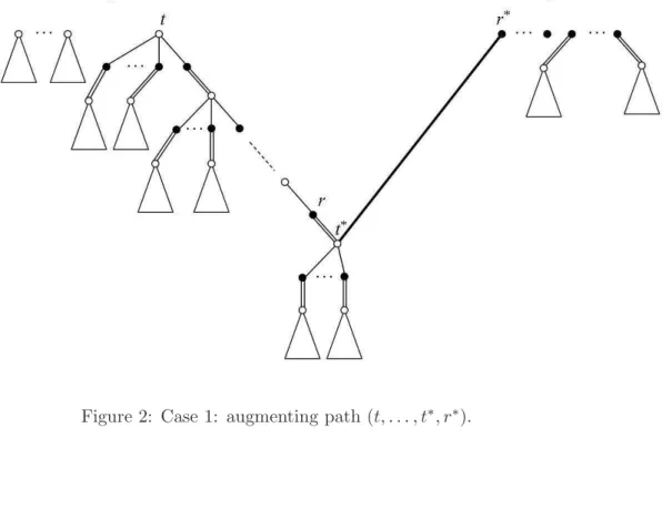
• robot vertex r∗ is free (unmatched). In this case there is an augmenting path
(t, . . . , t∗, r∗) starting from a (free) root target vertex t of F1
, connected with t∗
through an alternating path of F1
, and ending in r∗ through edge (t∗, r∗). Figure 2 shows this case, where white dots are target vertices, black dots are robot vertices, plain line segments are free edges, double line segments are matched edges, and the bold line segment is the new admissible edge (t∗, r∗); triangles represent subtrees
rooted at target vertices. By exchanging the free and matched edges in the aug-menting path we get the augmented matching. Since target vertex t is not free any more, the whole tree of F1
rooted in t moves to F2
and is connected to root r∗ over t∗ (see Figure 3).
[Insert Figure 2 around here] [Insert Figure 3 around here]
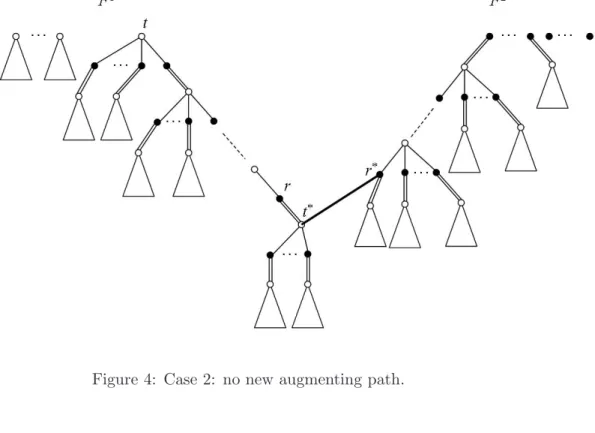
• robot vertex r∗ is not free, i.e., it is matched. In this case there is no new augmenting
path (see Figure 4); the two forests of alternating trees are updated by disconnecting robot vertex r∗, along with the whole subtree rooted in r∗, from forest F2
, and connecting this subtree (rooted in robot vertex r∗) to the target vertex t∗ in forest
F1
through the new admissible edge (t∗, r∗) (see Figure 5).
[Insert Figure 4 around here] [Insert Figure 5 around here]
Note that at the end, when we have a perfect matching of ¯G, all target vertices are matched and therefore forest F1 is empty.
4.3.1 Implementation details
The robots interactively execute the steps of the algorithm based on the local information and the one received through the messages from their neighbors in a communication graph.
The structure of the communication graph is made of the forests F1
and F2
restricted to robots. The interconnected robots recalculate the structure of the forests each time the forests change. Therefore, the connection graph is updated each time the update of the forests F1
and F2
occurs.
Each robot r keeps in its memory 4 pointers relating to the robots on its neighboring positions in the forests, i.e., the father robot, the oldest son robot, the next older brother robot, and the next younger brother robot, as seen from Figure 6. The first two pointers are used to move upwards and downwards in the forest while the two latter ones are used to explore the branch.
[Insert Figure 6 around here]
Each robot r in its memory also keeps the data about its position (whether it is in F1
or F2
), its matched target mr (if there is none, i.e., if r is free, mr = 0), and the father
target vertex in the forest. Each robot r memorizes also the vector of the distances γrt
from the location of robot r to the targets’ locations, the value of the dual variable βr,
and the minimum slack value σr along with the target tr which obtains the σr.
Through autonomous calculations and the communication with the (robot) neighbors, robots get and share the information about the position of each target (whether in F1 or
F2
), the values of dual variables αtof all the targets t, the value of δ for the dual variables’
update, the new admissible edge (r∗,t∗) between a robot r∗ in F2
and a target t∗ in F1
due to the dual variables’ update, and the root robots r(F1
) and r(F2
) of forests F1
and F2
respectively (the first robot vertex in a depth-first search of the forest). All these data are locally stored by each robot. In this way, there is no common coordinator or a shared memory of the robots’ system.
In detail, the robots, depending on their positions in the forests, (e.g., whether they are in the augmenting path, in forest F1 or F2, etc.) change their roles, and accordingly do
some of the steps of the distributed Hungarian algorithm. In the following we describe the robots actions according to their roles.
Initialization (done by each robot r):
t, and βr := mint{γrt}.
• Initialize the pointers in such a way that robot r is connected only with its next older brother robot (r − 1) and next younger brother robot (r + 1) and has no father and no sons. This means that the forests are initialized as described in Section 4.3.
• Each robot positioned in F2
determines [σr, tr] without exchanging any message
with the others. Root robots r(F1
) and r(F2
) start the message exchange based on depth-first search (DFS) along the forests F1 and F2, respectively, asking if there is a free robot. In the contact
with the first free robot, the same informs r(F2
) to start a new iteration. In the following we describe the actions of the robots in respect to their roles during each iteration.
• Calculating [δ, (r∗, t∗)]. All the robots r ∈ F2
participate in calculating [δ, (r∗, t∗)].
The calculation of δ starts from the root robot r(F2
) and follows via the exchange
of messages through DFS of F2
. When the values of [δ, (r∗, t∗)] are found, the
information is transmitted to all the robots in F2 through message exchange based
on DFS starting from the root robot of F2
. The same DFS message passing applies to inform the robots in F1.
• Dual variables updating. All the robots r do the following: for each target t ∈ F1
set αt := αt− δ; moreover, if robot r belongs to F1, set βr := βr− δ. No messages
are exchanged in this phase.
• The father robot of t∗ (if any), returns the information about himself and about his
oldest son to all the robots through the DFS message passing.
• Root robot r(F2
) informs r∗ in F2
to start the next phase of augmenting or non augmenting the path.
• Augmentation. If r∗ is free (see Figure 2), then it initiates the augmentation of the
matching. Over the message passing from r∗and the robots in the augmenting path, robot r∗orders the swapping of the free and the matched edges along the augmenting
path. It sends the messages to the robots in F2
(through DFS message passing in F2
, starting from robot r(F2
the subtree of target t∗ in F1
. The information contains t∗, and all the objects in
the tree going backwards in F1
up to the first target t without robot father along the augmenting path (t, . . . , t∗, r∗). The robots simultaneously update the matching in respect to the messages received from r∗ and update the pointers to the adjacent
robots so that the tree of t∗ in F1
rooted in t moves to F2
and gets connected to root r∗ over t∗ (see Figure 3). The robots through the DFS message passing get the
updated information regarding the position of the targets in respect to the forests. Each robot r positioned in F2
calculates the new [σr, tr] without exchanging any
messages with the others.
• No Augmentation. If r∗ is already matched (see Figure 4), then it does not augment
the matching. It sends the message to r(F2
) to inform, through the DFS message passing, all the robots r in F2
to decrease minimum slack values σr by δ; r∗
dis-connects from forest F2
attaching itself together with its subtree to F1
over t∗ (see
Figure 5). Each robot r in F2
updates the new [σr, tr] data comparing the old value
of minimum slack σr with the slack value (γrt+ αt− βr) for each target t in the
subtree routed at r∗ in F1, which results in O(n2) exchanged messages.
The total computational time is O(n3
) as well as the total number of messages ex-changed by the robots; nonetheless, the computational time required to perform the lo-cal lo-calculation by each robot is O(n2
). Therefore, differently from other known distributed algorithms for the assignment problem recalled in Section 2, the proposed algorithm runs in strongly polynomial time.
Regarding the robustness of the proposed method, if the robot during the execution of the algorithm stops responding, it is considered erroneous and is eliminated from the further calculations. In the case where the robot was unmatched in the forest F2
, the cal-culation continues without any modifications, ignoring the robot in question. Otherwise, the algorithm starts from the beginning excluding the same.
5
Simulation results
The robotic Multi-Agent System was simulated in the C language using the CPLEX 8.0 callable library for the solution of problems Pi of the upper level and was run on a PC
with a 2.2 GHz dual-core duo CPU and 4 GB of RAM.
The production system instances on which the simulation is demonstrated has P = 50 tasks (products). The number of time periods of the planning horizon is T = 100, with the duration of each period ∆t = 1. The external demand rate of product i is modeled as di(k) = ¯di· [1 + δdi(k)], for k = 1, . . . , T , where ¯di is the average demand rate of the
product produced by task i in the planning horizon and δdi(k) are values generated by an
ARMA(2,2) as in Example 2 of Gaalman (2006). In our numerical example, the average demand is ¯di = 5, for each product i.
The production system is simulated with the production executed by different number of robots, N . In order to cover a wide range of cases (from very highly congested to very low-congested), we consider the number N of robots in the range from 10 to 300.
¯
N = 250 is the number of robots for which the average production rate of the system ¯
NP1·T PP
i=1
PT
k=1ri(k) (approximately) equals the total average demand rate PPi=1d¯i.
The values of the unitary production costs are given for the whole planning horizon.
Notice that when the unitary backlog cost bi(k) is not large enough in respect to the
unitary manufacturing cost ci(k) and the robot hiring cost ρi(k), it may happen that,
even if the system has enough capacity to clear all the demand, a positive backlog is found at the end of the planning horizon. For this reason, in the numerical case considered here, we assume for each task (product) i the following relation among the parameters of the cost function:
hi(k) ≤ ci(k) +
ρi(k)
ri(k)
≤ bi(k) (18)
According to (18), the demand is fulfilled if there are enough production resources avail-able, and, therefore, backlog at the end of the planning horizon can be used as a mea-surement of congestion. For simplicity we assume that the unitary costs of backlog, bi(k),
inventory, hi(k), manufacturing, ci(k), and robot rental, ρi(k), are constant and equal
for all the tasks in all the time periods. In particular we assume hi(k) = 4, ρi(k) = 4,
ci(k) = 1, and bi(k) = 5 ∀i, ∀k.
Finally, the robot production capacity ri(k) is also assumed to be constant and equal
for all the tasks and time periods. In particular, we assume ri(k) = 1 for each task i and
time period k. In this way, all the considered mixed integer problems are solved within a fraction of one second by CPLEX, and, hence, we are able to execute each simulation in
less than two minutes; notice, however, that providing a CPU time efficient approach for the considered scheduling problem is out of the scope of this paper.
For the analysis of the results, notice that the stopping criteria of the upper level decentralized algorithm are a maximum number of iterations, in our problem instance equal to 1000, and an error between the best upper and lower bound found, equal to 0.01 (whichever of those two is satisfied first). The performance of the decentralized model is evaluated with respect to that of the centralized optimization model with objective function being the sum of the objective functions (1) of problems Pi, subject to constraints
(2)–(5) for each i ∈ {1, . . . , P }, and constraint PP
i=1ni(k) ≤ N , for each k ∈ {1, . . . , T }.
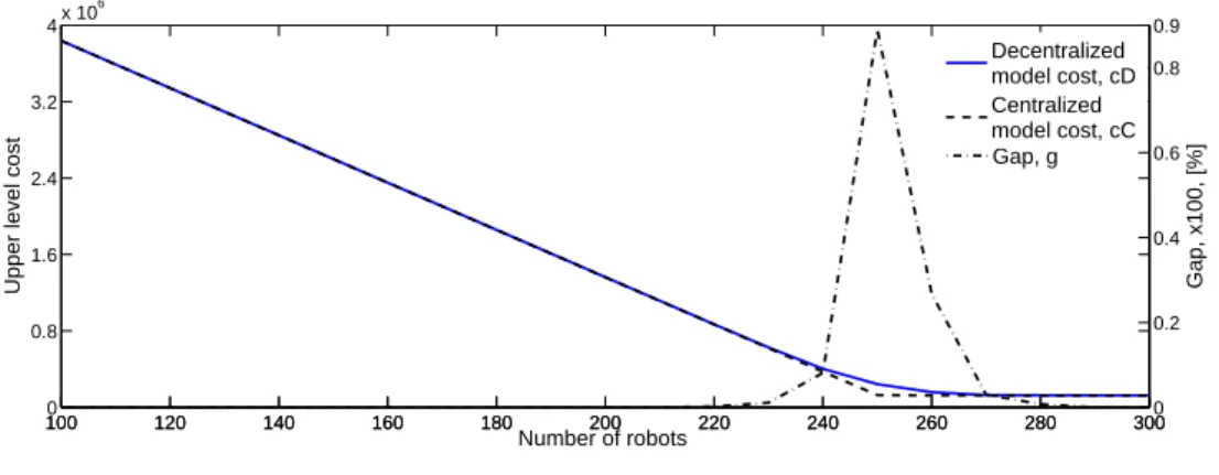
Let cD be the best solution value of the total production cost (social welfare)
ob-tained for the decentralized model by applying the proposed approach, and let cC be the
optimal solution value of the centralized one. Performance of the decentralized model in respect to the centralized one is evaluated measuring the relative gap (in percentage) g = [(cD− cC)/cC] · 100, that provides an estimation of the relative extra-cost incurred in
the decentralized model in respect to the centralized one for not having at disposal all the system information to optimally reconfigure and distribute the available robots.
In the simulation of the MRTA problem on the lower level of the pro-posed approach, we assume that the robots move within a convex regular
decagon with a circumscribed circle of radius rc = 100 with 10 production
cen-ters positioned on the vertices of the same, and with the given P = 50 (fixed) production machines (each one for each task) equally distributed on the 10 production centers, whose locations corresponds therefore to the task loca-tions ℓi (i = 1, . . . , 50). It is assumed that the robot depot is placed in the center of the
decagon, and all the robots are placed in the depot at the beginning, and have to turn back to the depot at the end of the production horizon, all traveling equal distances rc = 100
from the depot to their allocated task positions and vice versa. The time of the robots’ rearrangement and their traveling times from one position to another are negligible in respect to the duration ∆t of each period. When changing the production position from one task to another, the robots choose the shortest distance path. We do not enter here in the details of collision avoidance since it is not a subject of this paper.
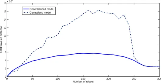
presents the solution of the lower level in terms of the total distance traveled by robots in correlation to the varying number of robots in the system.
[Insert Figure 7 around here] [Insert Figure 8 around here]
Since the total mean demand rate in each time period equals 250, the system with up to approximately N = 230 robots is very highly congested, and, as a result, by increasing the number of robots N from 0 up to 230, the total production costs linearly decrease since the prevailing are the costs due to the accumulated backlog and are of the same order for the centralized and decentralized model. In the range from 230 to 280 robots, the decentralized model sustains higher costs of production due to the lack of complete system’s information for the reconfiguration of the production resources. At N = 230, the relative gap between the decentralized and centralized model is 1%, after which it increases and has a peak value at N = 250, where the total robot production rate equals the total mean demand rate per period. This gap between decentralized and centralized model decreases with the less congested instances up to N = 270, where the gap falls to 3%. By further increasing the number of robots, at N = 288 the gap equals zero. Indeed, the maximum number of robots needed for both the centralized and decentralized model is N = 288. Increasing N beyond this number does not affect the solution value, as can be seen in Figures 7 and 8.
In fact, when the total number of robots in the system is significantly lower than ¯N , the system is highly constrained, and both the decentralized and the centralized approach are characterized by very high and comparable backlog costs. The total costs of the two approaches differ in practice in the values of the other cost components, that are indeed negligible in respect to the backlog cost. Oppositely, when the total number of robots in the system is significantly larger than ¯N , the local optimal solutions of the task agents’ subproblems are likely to satisfy (resource) constraints (6), and then the set of local solutions of the decentralized approach is equivalent to the centralized solution. Moreover, in this case, there is no backlog cost and the total cost of both approaches is
low. In the intermediate case, i.e., when N approaches ¯N , the gap g among the total
that the latter approach can take full advantage of having at disposal all the information, which allows it to satisfy the resource constraint with a lower backlog cost in respect to the one payed in the decentralized case.
On the second level, total distance traveled by the robots varies with N and follows approximately a bell shaped curve (as can be seen in Figure 8). Initially, the centralized model has a lower translocation cost for up to N = 30, after which the traveled distance of the centralized model increases much more rapidly than the one of the decentralized model. In the congested instances where 230 < N < 280, robots in the centralized model travel up to 3 times more than the ones in the decentralized case. This is where the centralized model seeks to diminish the total production cost by better reallocating the robots having all the system’s information at disposal.
Since, on the upper level, the decentralized model is more costly and gives no better results than the centralized one due to the lack of complete system’s information in the decision processes of individual agents, and because of the additional cost λ which each task has to pay in the negotiation for acquiring the robots, the system is not as flexible and the robots do not change production positions as frequently as in the centralized system. On the second level, this lack of flexibility results, in general, in inferior required total movement distance of the robots’ reallocation as seen from Figure 8.
6
Conclusion
In this paper, a dynamic factory layout with a set of mobile production resources (e.g. robots) carrying out the production, has been proposed. Notice, however, that the latter can also be used to increment the production capacity of already existing machines in the traditional factories. In respect to a classical layout where the production locations are placed on static positions, a less constrained facility is obtained, which allows to postpone critical design decisions to the operative level and makes the plant more capable of responding to a fluctuating external demand. The proposed solution can be considered as an extension of traditional factories since every control policy implemented in plants with a static layout can be applied in the dynamic factory proposed in this paper, while the viceversa is not true.
each period of the planning time horizon, the determination of the robots’ positions in order to minimize all the production costs. Owing to this complexity, and/or also for the inherent decentralized structure of the system, a two-level decentralized multi-agent system (MAS) production scheduling architecture was proposed: at the first level the agents are the tasks which compete for the robots, and at the second level the agents are the robots which reallocate themselves among different tasks to satisfy the requests coming from the first level. An iterative auction based negotiation protocol was used at the first level while the second level resolves a Multi-Robot Task Allocation Problem (MRTA) through a distributed version of the Hungarian Method.
The advantages of the decentralized architecture with respect to the centralized one were discussed in the paper and include robustness and efficiency (notice that the decen-tralized approach can be in some cases the only viable solution for the structural organi-zation of the system). From the simulation results it can be observed, however, that the lack of information associated with the decentralized solution implies larger production costs, with respect to the centralized approach when the system has a strict number of robots necessary to carry out requested production: in this case, in fact, the centralized approach is characterized by a much higher robot displacement distance with respect to the decentralized solution; the latter tending to under-utilize the production resources and representing a sub-optimal control policy.
Moreover, the proposed dynamic layout (even if sub-optimally controlled) shows a significant superiority with respect to a static plant, in particular if the fluctuation of the demand is characterized by low frequency components or by a drift in the average demand: in these cases, in fact, the strategic static sizing of the plant (i.e. the decision on the number of machines which must be dedicated to a particular product) may result completely inappropriate for long time periods, while a dynamic solution with mobile production robots adequately adapts their roles and positions in the plant to track the perturbations.
References
Barahona, F., Anbil, R., 2000. The volume algorithm: producing primal solutions with a subgradient method. Math. Prog. 87, 385–399.
Bertsekas, D.P., Castanon, D.A., 1989. The auction algorithm for the transportation problem. Ann. Oper. Res. 20, 67–96.
Bertsekas, D.P., 1991. Linear Network Optimization: algorithms and codes, MIT Press, Cambridge, USA.
Bertsekas, D.P., 1992. Auction algorithms for network flow problems: A tutorial intro-duction. Comput. Opt. and Appl. 1(1), 7–66.
Bertsekas, D.P., Castanon, D.A., Eckstein, J., Zenios, S.A., 1995. Parallel computing in network optimization, In: Ball M.O. et al. (Eds.), Network Models – Handbooks in Operations Research and Management Science, Vol. 7. Elsevier, Amsterdam, The Netherlands, pp. 330–399.
Bischoff, R., Kurth, J., Schreiber, G., Koeppe, R., Albu-Sch¨affer, A., Beyer, A., et al., 2010. The KUKA-DLR Lightweight Robot arm – a new reference platform for robotics research and manufacturing, In: Proc. of ISR/ROBOTIK 2010.
Burkard RE, C¸ ela, E., 1999. Linear assignment problems and extensions, In: Du, D.Z., Pardalos, P.M. (Eds.), Handbook of Combinatorial Optimization, Vol 4(1). Kluwer Academic Publishers, Dordrecht, The Netherlands, pp. 221–300.
Buyya, R., Abramson, D., Giddy, J., Stockinger, H., 2002. Economic models for resource management and scheduling in grid computing. Concur. and Computat.: Pract. and Exper. 14, 1507–1542.
Chen, H., Chu, C., Proth, J.M., 1998 An improvement of the Lagrangean relaxation approach for job shop scheduling: A dynamic programming method. IEEE Trans. on Rob. and Autom. 14(5), 786–795.
Chevaleyre, Y., Dunne, P.E., Endriss, U., Lang, J., Lemaitre, M., Maudet, N., et al., 2006. Issues in multiagent resource allocation. Informatica 30(1), 3–31.
Christensen, J.H., 1994. Holonic manufacturing systems: Initial architecture and stan-dards directions, In: Proc. 1st Euro Workshop on Holonic Manufacturing Systems, Vol 14. HMS Consortium, Hannover, Germany.
Clearwater, S.H., 1996. Market-based control: a paradigm for distributed resource allo-cation, World Scientific Publishing Co. Inc., River Edge, NJ, USA.
Dias, M.B., Kannan, B., Browning, B., Jones, E.G., Argall, B., Dias, M.F., Zinck, M., et al., 2008. Sliding autonomy for peer-to-peer human-robot teams, In: Proc. of the 10th Internat. Conf. on Intel. Auton. Systems. pp. 332–341.
Dugnay, C.R., Landry, S., Pasin, F., 1997. From mass production to flexible/agile pro-duction. Int. J. of Oper. and Prod. Manag. 17, 1183–1195.
Florian, M., Lenstra, J.K., Rinnooy Kan, A.H.G. 1980. Deterministic Production Plan-ning: Algorithms and Complexity. Manag. Sci. 26(7), 669–679.
Frei, R., Ferreira, B., Di Marzo Serugendo, G., Barata, J., 2009. An architecture for self-managing evolvable assembly systems, In: Proc. of the IEEE Internat. Conf. on Systems, Man and Cybernetics. pp. 2707–2712.
Gaalman, G., 2006. Bullwhip reduction for ARMA demand: The proportional order-up-to policy versus the full-state-feedback policy. Auorder-up-tomatica 42(8), 1283–1290. Gerkey, B.P., Mataric, M.J., 2003. A framework for studying multi-robot task allocation,
In: Shultz, A.C. et al. (Eds.), Multi-robot systems: from swarms to intelligent automata, Vol. 2. Kluwer Academic Publishers, Dordrecht, The Netherlands, pp. 15–26.
Gerkey, B.P., Mataric, M.J., 2004. A formal analysis and taxonomy of task allocation in multi-robot systems. Int. J. of Rob. Res. 23(9), 939–954.
Giordani, S., Lujak, M., Martinelli, F., 2009. A Decentralized Scheduling Policy for a Dynamically Reconfigurable Production System. Lecture Notes in Artificial Intelli-gence 5696, 102–113.
Giordani, S., Lujak, M., Martinelli, F., 2010. A distributed algorithm for the multi-robot task allocation problem. Lecture Notes in Artificial Intelligence 6096, 721–730.
Hawes, N., Hanheide, M., Sj¨o¨o, K., et. al., 2010. Dora The Explorer: A Motivated
Robot, In: Proc. of 9th Int. Conf. on Auton. Agents and Multiagent Systems (AAMAS 2010).
Held, M., Wolfe, P., Crowder, H.D., 1974. Validation of subgradient optimization. Math. Prog. 6(1), 62–88.
Helms, E., Schraft, R.D., Haegele, M., 2002. Robwork: Robot assistant in industrial environments, In: Proc. of the 11th IEEE Int Workshop on Robot and Human interactive Communication, ROMAN2002. Berlin, Germany, pp. 399–404.
Huang, P.Y., Chen C.S., 1986. Flexible manufacturing systems: An overview and bibli-ography. Prod. and Inv. Manag. 27(3), 80–90.
Kraus, D.S., 2001. Strategic negotiation in multiagent environments, MIT Press, Cam-bridge, MA, USA.
Kuhn, H.W., 1955. The Hungarian Method for the Assignment Problem. Nav. Res. Log. Quart. 2, 83–97.
Kurose, J.F., Simha, R., 1989. A microeconomic approach to opt resource allocation in distributed comp systems. IEEE Trans. on Comp. 38(5), 705–717.
Kutanoglu, E., Wu, S.D., 2006. Incentive compatible, collaborative production schedul-ing with simple communication among distributed agents. Int. J. of Prod. Res. 44(3), 421–446.
Kwok, K.S., Driessen, B.J., Phillips, C.A., Tovey, C.A., 2002. Analyzing the multiple-target-multiple-agent scenario using optimal assignment algorithms. J. of Intl. and Rob. Sys. 35(1), 111–122.
Lueth, T.C., Laengle, T., 1994. Task description, decomposition and allocation in a distributed autonomous multi-agent robot system, In: Proc of the IEEE/RSJ/GI International Conference on Intl. Robots and Systems 94’: Advanced Robotic Sys-tems and the Real World. pp. 1516–1523.
Mun, J., 2002. Real options analysis: Tools and techniques for valuing strategic invest-ments and decisions, Wiley, Hoboken, NJ, USA.
Orlin, J.B, Stein, C., 1993. Parallel algorithms for the assignment and minimum cost flow problems. Oper. Res. Lett. 14, 181–186.
Papadimitriou, C.H., Steiglitz, K., 1982. Combinatorial optimization: algorithms and complexity, Prentice-Hall Inc., Englewood Cliffs, NJ, USA.
Reiser, U., Connette, C., Fischer, J., et. al., 2009. Care-O-bot 3: creating a productR
vision for service robot applications by integrating design and technology, In: Proc. of the 2009 IEEE/RSJ international conference on Intelligent robots and systems. pp. 1992–1998.
Roundy, R.O., Maxwell, W.L., Herer, Y.T., Tayur, S.R., Getzler, A.W., 1991. A price-directed approach to real-time scheduling of production operations. IIE Transactions 23(2), 149–160.
Schneider, J., Apfelbaum, D., Bagnell, D., Simmons R., 2005. Learning opportunity costs in multi-robot market based planners, In: Proc. of 2005 IEEE International Conference on Robotics and Automation. pp. 1151–1156.
Selim, H.M., Askin, R.G., Vakharia, A.J., 1998. Cell formation in group technology: review, evaluation and directions for future research. Comp. and Ind. Eng. 34(1), 3–20.
Sellner, B., Heger, F.W., Hiatt, L.M., Simmons, R., Singh, S., 2006. Coordinated multi-agent teams and sliding autonomy for large-scale assembly, In: Proc. of the IEEE, Vol. 94(7). pp. 1425–1444.
Shen, W., Hao, Q., Yoon, H.J., Norrie, D.H., 2006. Applications of agent-based systems in intelligent manufacturing: An updated review. Adv. Eng. Informatics 20(4), 415–431.
Shen, W., Hao, Q., Wang, S., Li, Y., Ghenniwa, H., 2007. An agent-based service-oriented integration architecture for collaborative intelligent manufacturing. Rob. and Comp. Int. Man. 23(3), 315–325.
Smith, S.L., Bullo, F.. 2007. Target assignment for robotic networks: Asymptotic per-formance under limited communication, In: Proc. of American Control Conference 2007 (ACC’07). New York, USA, pp. 1155–1160.
Sugar, T., Kumar, V., 2000. Control and coordination of multiple mobile robots in manipulation and material handling tasks, In: Proc. of the Sixth International Symposium on Experimental Robotics. Springer-Verlag, pp. 15–24.
Sycara, K.P., 1998. Multiagent Systems. AI Magazine 19(2), 79–92.
Tan, J.T.C., Duan, F., Zhang, Y., Watanabe, K., Kato, R., Arai, T., 2009. Human-robot collaboration in cellular manufacturing: design and development, In: Proc. of the 2009 IEEE/RSJ Internat. Conf. on Intell. Robots and Systems. IEEE Press, pp. 29–34.
Wang, C. and Ghenniwa, H., Shen, W., 2008. Real time distributed shop floor scheduling using an agent-based service-oriented architecture. Int. J. of Prod. Res. 46(9), 2433–2452.
Wooldridge, M., 2002. Introduction to multi-agent systems, John Wiley and Sons, Hobo-ken, NJ, USA.
Zavlanos, M.M., Spesivtsev, L., Pappas, G.J., 2008. A distributed auction algorithm for the assignment problem, In: Proc. of 47th IEEE Conf. on Decision and Control. Cancun, Mexico, pp. 1212–1217.
Figure 1: Two-level framework for multi-agent system production planning and scheduling of mobile robots.
Figure 2: Case 1: augmenting path (t, . . . , t∗, r∗).
Figure 4: Case 2: no new augmenting path.
Figure 6: The pointers to the (robot) neighbors of a robot j. 1000 120 140 160 180 200 220 240 260 280 300 0.8 1.6 2.4 3.2 4x 10 6
Upper level cost
100 120 140 160 180 200 220 240 260 280 3000 0.2 0.4 0.6 0.8 0.9 Number of robots Gap, x100, [%] Gap, g Decentralized model cost, cD Centralized model cost, cC
0 50 100 150 200 250 300 0 2 4 6 8 10 12 14 16 18x 10 5 Number of robots
Total traveled distance
Decentralized model Centralized model
Figure 8: Distributed vs. centralized MRTA dynamic model, total distance traveled by robots.