Radio Morphing:
towards a fast computation of the radio signal from air showers
Anne Zillesa, Olivier Martineau-Huynhb,c, Kumiko Koteraa, Matias Tuerosg, Krijn de Vriese, Washington Carvalho Jr.d, Valentin Niessf, Nicolas Renault-Tinaccia, Valentin Decoenea
aSorbonne Université, UPMC Univ. Paris 6 et CNRS, UMR 7095, Institut d’Astrophysique de Paris, 98 bis bd Arago, 75014 Paris, France bLPNHE, CNRS-IN2P3 et Universités Paris VI& VII, 4 place Jussieu, 75252 Paris, France
cNational Astronomical Observatories, Chinese Academy of Sciences, Beijing 100012, China dUniversidade de Santiago de Compostela, 15782 Santiago de Compostela, Spain eVrije Universiteit Brussel, Physics Department, Pleinlaan 2, 1050 Brussels, Belgium
fClermont Université, Université Blaise Pascal, CNRS/IN2P3, Laboratoire de Physique Corpusculaire, BP. 10448, 63000 Clermond-Ferrand, France gInstituto de Física La Plata - CONICET/CCT- La Plata. Calle 49 esq 115. La Plata, Buenos Aires, Argentina
Abstract
Over the last years, radio detection has matured to become a competitive method for the detection of air showers. Arrays of thousands of antennas are now envisioned for the detection of cosmic rays of ultra high energy or neutrinos of astrophysical origin. The data exploitation of such detectors requires to run massive air-shower simulations to evaluate the radio signal at each antenna position. In order to reduce the associated computational cost, we have developed a semi-analytical method for the computation of the emitted radio signal called Radio Morphing. The method consists in computing the radio signal of any air-shower at any location from the simulation of one single reference shower at given positions by i) a scaling of the electric-field amplitude of this reference shower, ii) an isometry on the simulated positions and iii) an interpolation of the radio pulse at the desired position. This technique enables one to compute electric field time traces with characteristics very similar to those obtained with standard computation methods, but with computation times reduced by several orders of magnitude. In this paper, we present this novel tool, explain its methodology, and discuss its limitations. Furthermore, we validate the method on a typical event set for the future GRAND experiment showing that the calculated peak amplitudes are consistent with the results from ZHAireS simulations with a mean offset of +8.5% and a standard deviation of 27.2% in this specific case. This overestimation of the signal strength by Radio Morphing arises mainly from the choice of the underlying reference shower.
Keywords: radio detection, high-energy astroparticles, air-shower simulation, radio-signal parametrization c
2019. This manuscript version is made available under the CC-BY-NC-ND 4.0 license http://creativecommons.org/licenses/by-nc-nd/4.0/
1. Introduction
An extensive air-shower develops when a primary high-energy cosmic particle interacts with molecules in the atmosphere, generating a cascade of secondary parti-cles. The electrons and positrons in the shower produce coherent, broadband and impulsive electromagnetic sig-nals, that can be detected in the tens to hundreds of MHz frequency range.
Radio impulses from air-showers have been known and measured since 1960s, but it was only in the last
Email address: zilles@iap.fr(Anne Zilles)
decades, thanks to the developments in digital signal processing, that this domain experienced a rebirth as a promising astroparticle detection technique [1, 2, 3]. The results of for example AERA (Auger Engineering Ra-dio Array) and Tunka-Rex (Tunka RaRa-dio Extension) on the energy reconstruction of the primary particle [4, 5] and the latter and LOFAR (LOw Frequency ARray) on the measurement of the mass composition [6, 7] show that radio detection has become competitive with stan-dard methods such as fluorescence light. Where LOFAR and AERA used a scintillator-based trigger, autonomous detection by a self-triggered radio detection set-up was
successfully shown by TREND last year [8], and ear-lier already by the ARIANNA [9] and ANITA [10] ex-periments while the AERA experiment also recorded self-triggered radio event identified as EAS signal by co-incidence with the Auger Surface Detector [11]. These successes are due to drastic technological advances, but also to the considerable progress made in the understand-ing and modelunderstand-ing of the radio emission mechanisms of air showers.
Both macroscopic and microscopic approaches can be found in the literature to model the radio-emission of air-showers. The former are mostly analytical and are based on the modeling or fitting of the global physical effects that contribute to the radio emission from exten-sive air-showers (e.g., [12, 13, 14, 15, 16]). The latter are numerical simulations that treat particles in the air-shower individually, and compute their electromagnetic radiation from first principles. Uncertainties then stem from the calculation of the air-shower itself. Several sim-ulation codes exist on the market with different levels of complexity, e.g., SELFAS [17], MGMR [15], EVA [18], CoREAS [19], ZHAireS [20]. In the last years their results have started to converge, and were found to be consistent with radio-signal measurements taken under laboratory conditions [21] and with air-shower arrays [22, 23].
Macroscopic approaches are fast –being analytical–, and enable one to grasp a physical insight on the various features of the radio signal, that are not yet fully under-stood. But they also have serious limitations, when one wishes for example to study the signatures expected for specific instrument layouts. Detailed spatial, spectral and temporal structures of the signal can be easily lost in the process of integrating over different contributions and due to simplifying geometrical assumptions. Besides, these formalisms contain free parameters to be tuned, such as the drift velocities, which strongly impacts the predicted electric field strengths [15].
On the other hand, running microscopic simulations for very high-energy particles and very large or dense arrays consisting of hundreds of antennas, is highly time-consuming, so that one quickly reaches the limitations of the computational resources. Typically, simulating the electric-field traces over 200 radio antennas for one air-shower of primary energy 1017eV with the ZHAireS simulation costs about 2 hours on one node and with a thinning level of 10−4. In the early phases of an ex-periment, when exploring the performances of particular layouts, a more portable and faster method is needed, that also provides as precise information than the classical models that have been studied so far.
This can be achieved by Radio Morphing, a novel
method we present in this paper. It consists in simulat-ing the radio signal emitted by one generic air-shower and in morphing of it in order to obtain the electric field from any primary particle, at any desired antenna po-sition. Morphing is performed by using mostly well-documented analytical formalisms which enable to ac-count for the effect of each relevant primary particle, as well as atmospheric conditions and detector position parameters.
Our approach allows us to reflect the complexity of the particle distributions in spite of the analytical layer, thanks to the use of the initial full simulation output. The morphing treatment allows fast calculations. For the example given above, once a single generic shower simulation has been generated, the response over 200 radio antennas can be computed in less than 2 minutes with Radio Morphing on one node: a gain of roughly 2 orders of magnitude in CPU time. The gain further increases for lower thinning levels.
We first recall in Section 2 the basics of radio-emission. Section 3 details the physical principles behind the construction of the Radio Morphing method, and outlines the full Radio Morphing method. We demonstrate in Section 4 the performances of the method in reproducing the key features of radio-emission from air-showers, and compare our results with microscopic simulation outputs for a set of horizontal events which are expected to be measured by the future GRAND detector [24]. We discuss possible improvements and limitations originated from assumptions made for simplicity in Section 5.
The Radio Morphing method discussed in this paper has been implemented as a dedicated Python module [25], freely available online under the LGPL-3.0 license. The radiomorphing module requires numpy [26] in order to speed up intensive numerical computations, e.g. matrix operations or Fourier transforms.
2. Physics of radio emission
A primary high-energy particle induces an extensive air-shower in the atmosphere of the Earth, i.e., a cascade of high-energy, mostly leptonic, particles and electromag-netic radiation. Most of the particles are concentrated in a shower front, that is typically a few centimeter to meters thick near the shower axis. Time variation of the total charge or current in the relativistic shower front in combination with Cherenkov effects leads to coherent radio emission over the typical dimensions of the par-ticle cascade. These radio pulses last typically tens of nanoseconds, with varying amplitudes of up to several
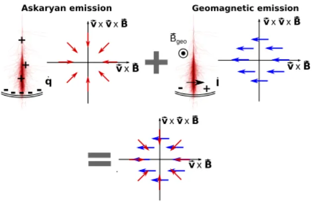
hundreds of µV/m. The signal can be interpreted by two main mechanisms (see figure 1).
The so-called Askaryan effect [27, 28] results from Compton scattering while the shower propagates through the Earth atmosphere. The resulting electrons are swept into the shower front. In a non-absorptive, dielectric medium the number of electrons in the particle front, and therefore the net charge excess in the cascade, varies in time, which induces a coherent electromagnetic pulse. The radio signal emitted by this mechanism is linearly polarized. The electric field vector is oriented radially around the shower axis, so the orientation of the electric field vector depends on the location of an observer with respect to the shower axis.
The second and main mechanism at play is the ge-omagnetic effect [14, 1]. In the shower front, the sec-ondary electrons and positrons are being deflected to-wards opposite directions by the geomagnetic field, after which they are stopped by interactions with air molecules. In total, this leads to a net drift of the electrons and positrons in opposite directions as governed by the Lorentz force ~F= q~v × ~B, where q is the particle charge, ~v the velocity vector of the shower and ~B the geomag-netic field vector. As these “transverse currents” vary in time during the air shower development, they lead to the emission of electromagnetic radiation. The polariza-tion of this signal is linear, with the electric field vector aligned with the Lorentz force (along ~v × ~B).
Depending on the position of the observer and hence the orientation of the electric field vector for the two emission mechanisms, these contributions can add con-structively or decon-structively, leading to an asymmetric ring structure: a radio footprint, the pattern of the radio signal on ground.
Since the refractive index of air is slightly larger than 1, the radio waves travel slower through the air than the relativistically moving particle front. In addition to a strong forward-beaming of the emission, this leads to a so-called Cherenkov compression. At particular ob-server positions on ground, a radio pulse is detected as being compressed in time since the radiation emitted by a significant part of the shower arrives simultaneously. The pulse becomes very narrow and coherent up to fre-quencies in the GHz region.
These observer positions can be found on the Cherenkov ring[29, 30, 31], given by cosΘC= (n β)−1 withΘCdefined as the Cherenkov angle, n the refractive index of the medium that depends on the emission height, and β the particle velocity.
One of the main observables that characterize the air-shower is the atmospheric depth Xmax(also called the shower maximumand given in g.cm−2) at which the
de-- + I Bgeo Geomagnetic emission v x v x B v x B -+ + - q + Askaryan emission v x v x B v x B v x v x B v x B
Figure 1: Main radio emission mechanisms in an extensive air-shower and the polarization of their corresponding electric field in the shower plane. The Askaryan effect can be described as a variation of the net charge excess of the shower in time ( ˙q) and the geomagnetic effect results from the time-variation of the transverse current in the shower ( ˙I). Both mechanisms superimpose, resulting in a complex distribution of the electric field vector (bottom).
velopment of the cascade reaches its maximum particle number in the electromagnetic component [32]. Since the strength of the emitted radio signal scales linearly with the number of electrons and positrons, and since the signal is strongly beamed forward, Xmaxcan be con-sidered at first approximation, as a point-source position, where the maximum radiation comes from. This approxi-mation is just valid in the far-field, and restricts therefore the methods to it.
3. The Radio Morphing method
Previous macroscopic studies have shown that the average radio emission properties from air-showers de-pends on a limited set of parameters, describing the en-ergy and geometry of the shower [12, 13, 14, 15, 16]. Following this observation, we have developed the Radio Morphing method, in which radio signals are rescaled from a single reference air-shower, via a series of simple mathematical operations.
This idea relies on the universality of the distribution of the electrons and positrons in extensive air-showers, that was pointed out by several works already [33, 34]. Interestingly, this distribution was found to depend mainly on the depth of the shower maximum Xmaxand the number of particles in the cascade at that depth, that is, on the age of the shower. Based on this concept, Ref. [35] presented a parametrization of the air-shower pair distributions, that enables one to calculate the prop-erties of any air-shower by a linear rescaling of a small number of parameters. The parametrization was later refined by, e.g., Refs. [36, 37].
Xmax
vxB v vx(vxB) Position along v x( v x B )-a xis (m)Position along vxB-axis (m) τ decay
θch
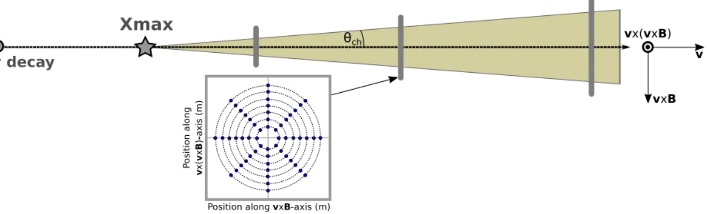
Figure 2: Sampling of the radio signal at several distances along the shower axis from the shower maximum Xmax. The antenna positions in the planes are arranged in a so-called star-shape pattern, defined by the shower direction ~v and the orientation of the Earth’s magnetic field ~B.
The distribution of these electrons and positrons in the shower front are directly responsible for the radio emission. Hence the associated radio signals are also expected to be universal. Because the radio signal is inte-grated over the full shower evolution, shower-to-shower fluctuations are further smoothed out for observer po-sitions in the far-field and this average universality can be seen as a robust estimate. Here, we would like to mention that for energies of electromagnetic showers of about 1020eV the Landau-Migdal-Pomeranchuk (LPM) effect which leads to a suppression of bremsstrahlung and pair production has to be taken into account [38]. Below the energy, the effect will not produce serious distortion in the shower development.
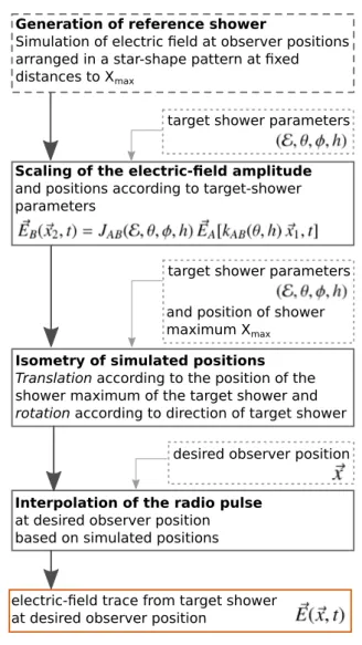
The strength of the measured radio emission is im-pacted by other external ingredients such as the geo-magnetic angle, and various geometrical distance scales (shower zenith angle and altitude) that can modify the distance of the observer to the radio source and thus stretch the size of the radio footprint on ground. First we focus on the generation of a reference shower in Section 3.1. We will demonstrate in Section 3.2 that, taking these mentioned processes into account, the radio emission properties can still be parametrized by only 4 parameters with a good level of precision at a fixed distance from the shower maximum Xmax, namely the primary particle energy E, the shower zenith and azimuth angles θ and φ at injection, and the shower injection alti-tude h. The direction and position of the shower can then be re-adjusted using isometries (Section 3.3). The last step is the performance of two-point interpolations (Sec-tion 3.4) of the electric field trace at the desired antenna position. Hence, we are able to calculate, at any desired observer positions, the electric field ~E(~x, t) emitted by any target shower from one generic simulated shower,
acting as reference, by simple analytical operations. The different steps of the Radio Morphing method are summarized in Fig. 3. The corresponding code is publicly available, see [25].
3.1. Sampling positions for the simulated radio signal In the simulation of radio emission from air showers the signals are recorded at a set of observer positions. To select these positions wisely, we profit from our knowl-edge about the emission mechanisms:
As mentioned in the previous section, the geomagnetic and the Askaryan effects are linearly polarized along ~v × ~B and around the shower axis, respectively. This nat-urally leads to a radiation profile that is not rotationally symmetric, and that can be adequately described in the shower-coordinate system defined by (~v, ~v × ~B,~v ×~v × ~B). The advantage of the shower coordinates is that the radio emission can be fully described by a superposition the two main emission mechanisms whose contributions can be disentangled due to their different polarizations.
A correct sampling of the radio signals has to record the lateral distribution of the radio signal as well as the longitudinal distribution function along the shower axis defined by ~v. In order to guarantee it while minimizing the number of simulated observer positions, the posi-tions are optimized so that at several distances from Xmax along the shower axis they cover the locations where the interference between the two radiation components reach their minima and maxima.
The variations in signal strength are along the ~v × ~ B-axis. We thus position a set of observers over a star-shaped patternin the shower plane with eight arms, two aligned with the ~v × ~Baxis, and two aligned with the ~v ×~v × ~B-axis (see figure 2) [39]. The extensions of these star-shape pattern in several distances from Xmaxare de-termined by the fact that the emission is strongly beamed
Generation of reference shower
Simulation of electric field at observer positions arranged in a star-shape pattern at fixed
distances to Xmax
Scaling of the electric-field amplitude
and positions according to target-shower parameters
Isometry of simulated positions Translation according to the position of the
shower maximum of the target shower and
rotation according to direction of target shower
Interpolation of the radio pulse
at desired observer position based on simulated positions
target shower parameters
desired observer position
electric-field trace from target shower at desired observer position
target shower parameters and position of shower
maximum Xmax
Figure 3: Recipe for Radio Morphing: These different steps are applied to a reference shower to receive the electric field traces for a target shower with desired parameters at the desired observer positions.
forward and forms a cone of a few degree opening angle with Xmax as an approximation for a point source (see Fig. 2).
In the following, reference showers are produced via microscopic simulations of the radio signal, performed in Cartesian coordinates, with the x-component aligned along magnetic North-South (NS), the y-component along East-West (EW) and the z-component pointing upward (Up), while the scaling procedure is performed in the shower referential defined by (~v,~v × ~B,~v × ~v × ~B). 3.2. Parametrizing the electric field
The radio signal measured at a given position ~xand time t can be formally described by the electric field vector ~E(~x, t). Four parameters constrain the strength
and polarization of the field at a given observer position: the primary’s energy E, the shower direction towards which the cascade is propagating1, defined by zenith θ and azimuth φ at injection, and the altitude of injection h. The key hypothesis in Radio Morphing is that, at a fixed distance to the shower maximum Xmax, the electric field vector of any shower B at the position ~xB can be derived from that of a reference shower A by a set of simple operations that are applied on the overall electric field ~EAand on the position ~xA
~
EB(~xB, t) = JAB(E, θ, φ, h) ~EA[kAB(θ, h) ~xA, t] , (1) where the scaling matrices JAB(E, θ, φ, h) and factors kAB(θ, h), can be calculated as a function of the refer-ence and target shower parameters (E, θ, φ, h), taking into account independent effects related to the primary energy, the geomagnetic field, the air density, and air re-fraction index. We detail in this section the dependency of the electric field on these various physical parameters at play in order to express JABand kAB.
We will derive their mathematical formulae by ex-pressing their dependency on the primary energy E, the geomagnetic angle α, the density ρ at the height of the shower maximum and the corresponding values for the Cherenkov angles ΘC of the target and the reference showers:
JAB(E, θ, φ, h)= jEjρjCJα (2) and
kAB(θ, h)= 1/ jC, (3)
where the scalars jE, jρ, jCand the matrix Jαwill be de-rived or explained below. The electric-field and position vectors will be written in the shower coordinate system (~v, ~v × ~B,~v × ~v × ~B).
3.2.1. Scaling in primary energy
Up to the frequencies corresponding to the typical thickness of the particle shower front (a few meters), secondary particles in the air-shower create a coherent radio emission: at a given frequency, the radiation emit-ted from several particle experiences negligible relative phase shifts during its propagation to the observer. This implies that the vectorial electric fields produced by each particle also add up coherently, and the total electric field amplitude scales linearly with the number of particles, itself scaling with E. We can thus write | ~E(~x, t)| ∝ E.
This relationship is consistent at first order with the seminal expression of the electric field amplitude derived
1In the conventional definition, azimuth and zenith are defined to describe the direction from which the shower is coming.
by [13] from pioneering measurements, and with the recent measurements performed by AERA and LOFAR [4, 6].
In practice, the electric-field amplitude of a generic shower A with primary energy EAcan be scaled to the one of a target shower B with the energy EB, by multi-plying by the factor
jE= EB
EA . (4)
Note that for frequencies typically higher than ∼ 100 MHz, coherence in the emission is no longer guar-anteed (besides for position in the Cherenkov cone, see Sec. 2) and can lead to uncertainties while applying this factor. More precisely, the effective thickness of the shower front that sets the coherence condition also de-pends on the observer angle.
3.2.2. Scaling in geomagnetic angle
The strength of the radiation emitted via the geo-magnetic effect scales with the strength of the Lorentz force ~F = q~v × ~B experienced by each particle in the shower front, and that induces a transverse cur-rent. The magnitude of the emitted signal scales with |~v × ~B| = |~v||~B| sin α, leading directly to a sinusoidal dependency of the electric field strength over the geo-magnetic angle: | ~E| ∝ |~v × ~B| ∝ sin α. Here, the ge-omagnetic angle is given by α = ](~v, ~B), introducing the dependency on the angles θ and φ of the shower. Also, this dependency is consistent at first order with the seminal expression of the electric field amplitude derived by [13] from pioneering measurements, and is confirmed experimentally by recent measurements per-formed by CODALEMA [40] and later by AERA and LOFAR [4, 6]. We neglect the linear dependency on the local magnetic field strength at the moment and choose a reference shower which is simulated for the target site. The amplitudes of reference shower A and tar-get shower B can be related via a scaling factor that takes into account the two geomagnetic angles α(θA, φA) and α(θB, φB) sensed by each shower: jα = sin α(θB, φB)/ sin α(θA, φA). This scaling was recently demonstrated experimentally by AERA [4].
Since the geomagnetic emission is linearly polarized along ~v × ~B, this factor is multiplied to the ~v × ~B compo-nent of the electric field in shower coordinates. Thus the scaling matrix can be expressed in the shower referential by Jα= 1 0 0 0 jα 0 0 0 1 with jα= sin α(θB, φB) sin α(θA, φA) . (5)
Here, we neglect the possible projection of the geo-magnetic component into the ~v component of the electric field, assuming that it is negligible with respect to our target accuracy. The phase shift between Askayran and Geomagnetic emission, as observed by LOFAR [41], is included implicitly by using a microscopic simulation as reference. We assume that the phase shift depends solely on the observed frequency and on the position of the observer with respect to the Cherenkov cone. There-fore, a scaling of the amplitude will not change the time difference, determined by the microscopic simulation.
For simplicity, we chose in the current version of Ra-dio Morphing to scale ~v × ~Bcomponent of the electric field without an a-priori decoupling of the contributions from the Geomagnetic and Askaryan effect. This impact of the latter one could be of order of a few % contribu-tion, depending on the measured polarization [42]. To exclude this artificially induced uncertainty, one has to decouple the two emission components completely, e.g. by comparing simulations with magnetic field turned on and off. These effects, as well as a possible scaling with the magnetic field strength, will be included in a future version of the Radio Morphing code.
3.2.3. Effects of air density
The parametrization on the injection altitude and zenith angles, and therefore on the air density, is poorly documented in the literature. Complicated ad-hoc fits have been invoked [43, 16], and the zenith scaling is han-dled at the moment in the community as a “distance to Xmax” correction. We present here a more natural model-ing of these effects, validated with ZHAireS simulations. In practice, our input parameter is the initial injection height h of the air shower, that corresponds to the altitude at which the shower starts developing in the atmosphere. Geometrically, this altitude is connected to the altitude of the shower maximum hXmaxby the following relation
via the zenith angle of the air shower θ at injection: hXmax = h + dhor/ tan θ (6)
with dhorthe horizontal distance of the shower maximum to the injection point of the shower. Here, a flat-Earth approximation can be used since dhor R⊗.
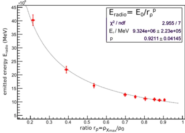
The dependency of the radiated energy on the den-sity at Xmaxis complicated to estimate analytically, as it corresponds to integrated values over the full shower development. We investigated this effect numerically using ZHAireS [20] simulations. We have produced sets of shower simulations with the parameters of the AERA [4] site at the Pierre Auger Observatory. The sets of simulations contain proton-induced showers with
energy 1017eV arriving from the North and a zenith an-gle θ = 80◦ in the conventional angular system used for cosmic rays. To achieve different densities at the position of the shower maximum, we changed the injec-tion height of the shower artificially. We calculated for each event the measured radiated energy on ground emit-ted by the shower. The result is illustraemit-ted in Figure 4. The errorbars are given by the RMS for 10 simulated air showers for each shower geometry. Interestingly, we find that the scaling of the radiated energy scales as | ~E|2∝ [ρXmax(h, θ)]
−1(for simplicity we use a value of 1 instead the exact fitting result), where ρXmax(h, θ) is the
air density at Xmax, related to the density at h via Eq. 6. This effect might be understood as follows. Each part of the footprint on the ground is more sensitive to a specific part of the longitudinal profile of the shower X. Thus if one “separates” each part of the footprint and links it to a specific position X in the profile, the electric field will scale with the air density at X. The integration over the energy in radio that reaches the ground, brings up an intricate convolution on the number of particles at each particular depth X, the air density at that depth and the position on the ground (each part is more sensitive to a certain X). Nevertheless, this effect is not yet fully understood and will be investigated further in a future study.
Even though we expect that the charge-excess in-creases with the air density, this effect is found to be relatively small. Therefore, we neglect it for the moment. In addition, the Askaryan emission is just a minor cor-rection to the total measured peak amplitude for inclined showers. For the reference shower used in Sec. 4.3,we found a relative contribution to the peak amplitude on the Cherenkov cone of about 14%. Therefore, we apply the scaling to all components of the electric field vector in the current version of Radio Morphing.
From these results, we can compute the scaling factor to obtain the amplitude of the target shower B from the reference shower A jρ= "ρ Xmax(hA, θA) ρXmax(hB, θB) #1/2 (7) with ρXmax(h, θ) the air density at altitude Xmaxfor
refer-ence and target showers A and B, related to the altitude at shower injection via Eq. 6. A comparison with the formula presented in Ref. [43] shows a nice agreement between the two formalisms, for highly inclined showers with high densities at the shower maximum.
3.2.4. Stretching effect from the Cherenkov angle The injection altitude and zenith angle also impact the size of the radio footprint. The opening angle of this
0.2 0.3 0.4 0.5 0.6 0.7 0.8 0.9 1 5 10 15 20 25 30 35 40 45 6 10 / ndf 2 χ 2.955 / 7 2.23e+05 9.324e+06 0.04145 0.9211 / ndf 2 χ 2.955 / 7 E0 9.324e+06 2.23e+05 p 0.9211 0.04145 Eradio= E0/rρp Eradi o (MeV) / MeV ratio rρ=ρXmax/ρ0 + -+ -emitted ener gy
Figure 4: Density scaling of the radio signal in the 30 − 80 MHz frequency band for a proton-induced showers with energy 1017eV arriving from the North. Red dots show the simulation outputs for an antenna array at the AERA site: the radiated energy in the radio signal Eradio as a function of the density ratio rρ= ρXmax/ρ0, with ρXmax the actual density at the height of the shower maximum and
ρ0 = 1.225 g/cm3 the density at sea level. The data points can be well-fit by a power-law function Eradio= E0/rρpwhere the values of E0and p are indicated in the label (dotted line).
cone depends on the altitude as the atmosphere becomes denser with decreasing height, leading to a larger refrac-tive index, and hence a larger Cherenkov cone. Indeed, the radius of the Cherenkov cone within which the ra-dio signal is emitted is given by rL = L tan ΘC where Lis the distance from Xmax andΘC = arccos[1/n(h)] is the Cherenkov angle [29, 30]. The refractive index nXmax(h, θ) is a function of the altitude h and zenith angle
θ and has to be evaluated at the altitude of the shower maximum Xmaxusing Eq. 6. For instance in ZHAireS, an exponential function is implemented [20].
The scaling between two showers at different injection heights is given by the ratio between the Cherenkov radii. This leads to a stretching factor for the radio footprints, to be applied to the positions ~xB= kC~xAwith
kC= ΘC,B ΘC,A ∼arccos[1/nXmax(hB, θB)] arccos[1/nXmax(hA, θA)] (8) with (hA, θA) and (hB, θB) the parameters of reference and target showers A and B. Here we have assumed that tanΘC ∼ ΘC, as ΘC 1. This means that the distances between the simulated antenna positions along the star-shaped arms are corrected by the corresponding stretching factor kC.
By energy conservation, the total radiated energy over each area intersecting the Cherenkov cone should be constant: | ~E(~x, t)|2/r2= constant, where r is the radius of the intersected area. The stretching of the area by rB = kCrAyields the following scaling factor between
Xmax (target) X
max (reference)
Figure 5: Illustration of the isometry operation: the simulated antenna positions for the reference shower (blue) are rotated and translated accordingly to the new shower direction (red line) and the Xmaxposition (yellow diamonds) of the target shower (red).
showers A and B jC= | ~EB(~x, t)| | ~EA(~x, t)| = 1 kC . (9)
Note that very deep showers can be affected by the clipping effect, when particles reach the ground before the shower has completely developed. This effect is not accounted for in the scaling of the electric-field ampli-tude.
3.3. Isometries of observer positions
Once the electric field vector of the reference shower ~
EA(~x1, t) has been morphed to ~EB(~x2, t) according to the set of parameters (E, θ, φ, h) of the target shower, we rotate and translate the positions, at which the signal was simulated, according to the new shower direction. This can be done straightforwardly by a rotation and a translation of observer positions in the star-shaped planes, where the electric field of the reference shower were sampled (see Section 3.1), as is illustrated in Fig. 5. The isometries performed on the ~EA(~xA, t) should (by definition) conserve the distance of each star-shaped plane to the position of Xmax. This condition is required in order to ensure the validity of the morphing process performed in the first step to account for the parameters (E, θ, φ, h).
The physical location in space of the target’s shower maximum Xmax depends on the actual shower param-eters, as e.g. the primary’s energy, as well as on the primary-particle type. It can be obtained from e.g. dedi-cated simulations of the induced particle cascade or be computed as follows: one integrates the traversed air density along the shower axis from the point of shower injection until the average depth of the shower maximum for the target shower is reached for this specific primary
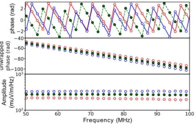
Frequency (MHz) 2 0 2 Frequency (MHz) 100 80 60 40 50 60 70 80 90 100 102 103 Frequency (MHz) phase (rad) Amplitude (muV/m/ Hz) unwrapped phas e (rad)
Figure 6: Example for the interpolation of phase (wrapped and un-wrapped) and amplitude for one antenna position: the red and blue markers represent the values at the antenna positions a and b which are used for the interpolation of the signal at the desired positions. Resulting phase and amplitude are represented by the green markers.
type, taking into account an atmosphere density model (e.g., an isothermal model).
3.4. Interpolation of the electric field traces: ~EA(xi, t) → ~
EA(x, t)
Once the electric field has been sampled at fixed an-tenna positions in the star-shaped planes, we interpolate the signal pulses at any desired position.
In the provided scripts for Radio Morphing, we im-plemented the method presented in [44] as an example for an interpolation of radio signals. Here, a Fourier transform into the frequency domain is performed, and the signal at a given location is obtained by a linear inter-polation in the frequency domain between two generic positions.
The signal spectrum can be represented in polar coor-dinates as
f(r, ϕ)= reiϕ
with r as the signal amplitude and ϕ the complex phase in the interval [−π, π). We detail in the following the two-point interpolation of r and ϕ at a given observer position.
The spectrum phase is wrapped into the interval [−π, π), which results in discontinuities at the interval limits, and to sawtooth-shaped features (see Fig. 6). Phases have to be unwrapped before interpolation, in order to account for data points sharing the same fre-quencies but with shifted phases that are not on the same saw-tooth edge. To locate the discontinuities the follow-ing conditions with i= 2, ..., n are scanned:
|ϕi−ϕi−1| > |ϕi−ϕi−1|+ π for ϕi< ϕi−1(10) |ϕi−ϕi−1| < |ϕi−ϕi−1| −π for ϕi> ϕi−1.(11)
For each discontinuity fulfilling these conditions, all the following data points ϕi+m are then corrected for a constant additive with l as the number of preceding discontinuities:
ϕi+m,new= ϕi+m+ 2πl . (12) This algorithm requires a sufficient sampling rate of the spectrum since the phase difference between consecutive data points has to be smaller than π. The unwrapping results in continuous phases can be interpolated linearly: ϕ(~x) = caϕ(~xa)+ cbϕ(~xb) . (13) Here, ~xis the observer position of the interpolated signal, and ~xa and ~xb the actual simulated observer positions. The weighting coefficients caand cbare defined as:
ca= ~xa−~x ~xb−~xa and cb= ~xb−~x ~xb−~xa
Since the amplitude in the frequency domain is in-dependent in each frequency bin, a linear interpolation within one bin is sufficient for r:
r(~x)= car(~xa)+ cbr(~xb) . (14) The interpolated spectrum is then given by
fint(r, ϕ)= r(~x) eiϕ(~x) (15) from which the corresponding time series can be derived via inverse Fourier transformation. An example for the interpolation of the phase and the amplitude is shown in figure 6.
The linear interpolation of the phases (see Eq. 13) implies a linear interpolation of the arrival time as long as the wave front can be estimated as a plane between two simulated observer positions, which is valid in the case of a dense grid of observers. This is a simplification of the hyperbolic shape of the wave front, that holds if the distance between the antennas is in the order of the wavelengths.
In the example presented in Section 4, the distances between the simulated antenna positions of the reference shower are larger than the radio wavelengths considered. In that case, the phase gradient in the phase interpolation cannot reproduce correctly the arrival timing of the signal at the considered antenna positions, while the signal structure itself is not affected. The correction of the arrival time of the signal at the observer position is part of foreseen developments for the Radio Morphing method.
10000 15000 20000 25000 30000 35000 40000 45000 50000 − 3000 − 2000 − 1000 0 1000 2000 3000 − 1500 − 1000 − 500 0 500 1000 1500 2000 2500 3000 surrounding planes desired position Xm ax position project ion on planes
V
line of s ight
Figure 7: Example for interpolation in 3D: after finding the two closest star-shape planes (red dots) to the desired antenna positions (blue circle), the projection of this position onto the planes along the line of sight are determined (green crosses). The 4 closest neighbored antenna positions which were simulated get identified (blue crosses). The yellow diamond represents the position of Xmaxfor that example shower.
3.4.1. 3D interpolation
The electric field time trace can be computed at any location inside the conical volume resulting from the isometry transformation. The process is the following, also illustrated on Fig. 7:
• First we define the intersection between the line linking the observer to the Xmaxposition and the two star-shape planes surrounding the observer position. • Then we compute the signal for each of these two in-tersection points from the closest neighbor’s signals through a bilinear interpolation, using the method detailed above.
• Finally, we interpolate these two signals in order to compute the time trace at the desired observer position.
The underlying hypothesis of this treatment is that the radio emission is point-like, and emitted from Xmax.
4. Comparison to microscopic simulation and per-formances
4.1. Time traces and frequency spectra
We validate the behavior of Radio-Morphed time traces and frequency spectra by a direct comparison to microscopic simulations for various antenna positions. As a reference shower we used an electron-induced air-shower with a primary energy of 0.1 EeV, an azimuth angle of 230◦and a zenith angle of 88.5◦(slightly up-going shower), injected at a height of 1700 m above sea-level. The radio emission was sampled in 5 km steps at several distances from the shower maximum. We sim-ulated the signal for 184 observer positions per plane
ZHAireS Radio Morphing
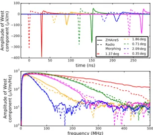
Figure 8: Example signal traces for an air shower induced by an electron with an energy of 1.05 EeV, an azimuth angle of 50◦and a zenith angle of 89.5◦(slightly up-going shower) using Radio Morphing (solid) and ZHAireS (dashed lines) for comparison. The antenna positions are in ∼ 75 km distance along the shower axis to the shower maximum while the Cherenkov ring is expected to be at an off-axis angle of ∼ 1.4◦. Top: Time traces of the West-East component of the electric field for antenna positions in different distances to the shower axis, given as off-axis angle, in the time domain. The time traces were shifted in time for a better comparison. Bottom: The corresponding frequency spectra.
arranged in the star-shape pattern, so that a conical vol-ume with a half-angle equal to 3◦is covered. A thinning level of 10−4and a sampling rate of 10 GHz were set for the simulation. The altitude is 2000 m above sea-level. The magnetic field direction is describe an inclination of 63.18◦and a declination of 2.72◦, having a magnetic field strength of 56.5 µT. As an atmosphere, we are us-ing the Linsley model includus-ing coefficients for the US standard atmosphere. These are the default options for all following ZHAireS simulations.
Figure 8 shows radio signals associated with a ZHAireS simulation (dashed lines) and Radio Morphing computation (solid lines) of an example target shower induced by an electron with energy of 1.05 EeV, first interaction at an height of 2200 m above sea-level, az-imuth angle of 50◦ (propagating towards North-West) and zenith angle of 89.5◦(slightly up-going shower). For the ZHAireS simulation a thinning level of 10−4was set. The signal is calculated for positions at several distances to the shower axis which are defined as an off-axis angle, located at a distance of roughly d = 75 km from the injection point of the shower. The bipolar characteristic of the signals is correctly reproduced in the time domain, and the signal amplitudes agree well with each other.
One can see that the time-compression of the signal
ZHAireS 45505560657075 44 46 48 50 52 54 56 58 South-North (km) 100 200 300 400 500 600 700 800 electric field ( V/m)μ RadioMorphing 45505560657075 44 46 48 50 52 54 56 58 West-East (km)
Figure 9: Comparison of the footprint detected by an antenna array, tilted by 5◦towards South: the peak amplitude distributions once simulated using ZHAireS (left) and once calculated by Radio Morphing (right) for the example target shower.
at the Cherenkov angle is also preserved by Radio Mor-phing. The Cherenkov ring is estimated to be located at ∼ 1.4◦from the shower axis, although this value strongly depends on the model used to calculate the refractive index nXmax at the altitude of Xmax. As expected, the
time traces and the frequency spectra both increase in amplitude at high frequencies when approaching the Cherenkov ring (red lines). A slight mismatch in signal amplitudes is observed for the position closest to the Cerenkov ring. This is very certainly due to statistical fluctuations in the shower development, which induce a difference between the Xmax value of the simulated shower compared to that computed with Radio Morph-ing (see Section 3.3). These different Xmaxvalues induce a (purely geometrical) variation of the Cherenkov ring radius at ground, only partially compensated by the dif-ferent values of the Cherenkov angle at different Xmax heights.
4.2. Peak amplitude distributions
Figure 9 shows the peak-amplitude distribution of re-ceived signals (West-East components) emitted by the same example target shower, simulated using ZHAireS (left) and calculated with Radio Morphing (right). The observer positions are located at a distance of roughly d = 75 km from the injection point of the shower on a slope slightly tilted by 5◦towards South. The antenna positions are arranged in a grid-like structure, as planed for the future GRAND experiment. The direct compari-son shows that for an extended array, the predictions for the signal strength by Radio Morphing and ZHAireS are in good agreement. The feature of the Cherenkov cone is clearly visible in both distributions.
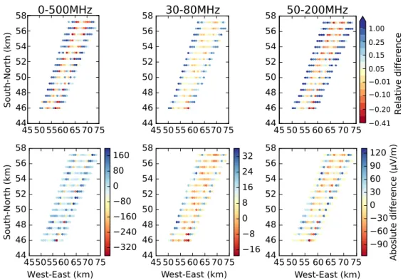
Figure 10 presents the relative and absolute dif-ferences between ZHAireS and Radio Morphed
foot-0-500MHz 45 50 5560 65 70 75 44 46 48 50 52 54 56 58 South -North (km) 45505560 6570 75 44 46 48 50 52 54 56 58 South -North (km) 320 240 160 80 0 80 160 West-East (km) 45 50 55 60 65 70 75 44 46 48 50 52 54 56 58 16 8 0 8 16 24 32 45 50 55 60 6570 75 44 46 48 50 52 54 56 58 30-80MHz 45 50 55 60 65 70 75 44 46 48 50 52 54 56 58 90 60 30 0 30 60 90 120 Abos lute d ifferen ce ( μ V/ m) 45 50 55 60 65 70 75 44 46 48 50 52 54 56 58 50-200MHz West-East (km) West-East (km)
Figure 10: The relative (top) and the absolute (bottom) differences in the West-East component of the signal distribution, defined as (ERM− EZHAireS)/EZHAireSand ERM− EZHAireS, for the full frequency band of 0 − 500 MHz (left) and for the frequency bands 30 − 80 MHz (center) and 50 − 200 MHz (right).
prints for this same example shower, defined as (ERM− EZHAireS)/EZHAireS(top) and ERM−EZHAireS(bottom), for the full frequency band of 0 − 500 MHz (left) and for the frequency bands 30 − 80 MHz (center) and 50 − 200 MHz (right). One can observe that the highest differences in the peak-amplitude distributions appear at the edges of the Cherenkov ring. This corresponds to the slight mis-match in the predicted positions of the Cherenkov cone discussed earlier. Since the signal strength drops sharply slightly off the cone angle, it leads to a larger difference in the predicted signal strength.
One observes that the signal predicted by Radio Mor-phing is slightly underestimated for observer positions on the Cherenkov ring, while it is slightly overestimated outside. This is induced mainly by the choice of the reference shower in this specific example, since a low-energy air shower with an low-energy of 0.1 EeV with a flat lateral distribution function acts as the reference for a target shower with an energy of 1.05 EeV. The discrep-ancy in the signal strength decreases if the time traces are filtered, as done for the 30 − 80 MHz (center) and 50 − 200 MHz (right) bands. Here, one first reason is the numerical noise at higher frequencies due to a low thinning level. Besides, coherence conditions are not fulfilled for frequencies above ∼ 100 MHz, so that the
linear scaling in energy induces larger uncertainties at higher frequencies.
4.3. Statistical validation of Radio Morphing
In the following, a comparison is made between results from Radio Morphing and ZHAires. The comparison is based on a set of ∼ 300 inclined air showers induced by high-energy electrons and pions that are propagating towards the North. The distribution in injection height above sea level, energy, zenith and azimuth are shown in Figure 11. Figure 12 shows the corresponding values for the geomagnetic shower and the determined contribution of the Askaryan emission to the peak amplitude at an ob-server position on the Cherenkov cone. For the reference shower, we can decouple the contribution from the Geo-magnetic and the Askayran emission for the simulated observer position along the positive ~v × ~B-axis due to the polarisation of the two signal contributions. We found an Askaryan contribution of about 14% for a position on the Cherenkov cone. Based on the given formula in [42], we calculate the expected relative contribution to the signal strength at this position by scaling with the ge-omagnetic angle. The overall assumption that the impact of the Askaryan emission is minor is also valid for the used event set. We computed the position of the shower
maximum Xmax of the target showers as described in Section 3.3. Here, we obtained the value for Xmax in g.cm−2from [45], while we determine the atmospheric column depth between the injection point and Xmaxof the electron (pion)-induced shower from the elongation rate value of photon (proton)-induced ones. The radio signals were computed at observer positions located inside the showers radio footprint, typically 40 − 50 km away from the shower injection point. Only observer positions with off-axis angles smaller than 1.6◦were considered.
The same reference shower as for the example above (see Sec. 4.2) was used to compute the Radio Morphed signals. Figure 13 displays the calculated peak-to-peak amplitude for each antenna position in the events derived with Radio Morphing versus the peak-to-peak amplitude from ZHAireS simulations. The antenna positions are arranged in a grid-like structure, as also used in Fig. 9.
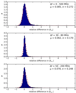
The green solid line marks equivalent amplitudes, the dashed and the dotted-dashed line 25% and 50% offsets, respectively. The distribution follows a linear trend, clus-tering along the diagonal. For most of the positions, the peak-to-peak amplitudes deviate by less than 25%. This demonstrates that Radio Morphing can reproduce the amplitudes at the same level of magnitude as ZHAireS. A histogram of the relative differences between the Radio Morphing and the ZHAireS peak-to-peak ampli-tudes at each antenna position is presented in Figure 14 (top). When excluding the values with relative di ffer-ences larger than 100% — only 1% of the total — the mean of the distribution, derived by a Gaussian fit, is µ = 8.5% with a standard deviation of σ = 27.2%. The Gaussian function with the mean and the standard devia-tion is plotted on top for comparison. It appears clearly that the function cannot describe the distribution properly due to a long asymmetric tail towards positive values. These entries arise mainly from the overestimation of the signal by Radio Morphing at antenna positions outside the Cherenkov ring as mention before. The fit does not have a quantitative value, but the plots aim to demon-strate qualitatively that Radio Morphing and ZHAireS agree within a reasonable margin. When the signals are filtered in the 30 − 80 MHz frequency range, then the mean and standard deviations decrease to µ= 6.2% and σ = 17.0% and to µ = 7.8% and σ = 24.8% after a filtering to 50 − 200 MHz, respectively. These behaviors are consistent with our observations in Figure 10.
5. Discussion
The previous section demonstrates the consistency between Radio Morphing and microscopic simulations.
Given that the method is built on simple mathematical operations, this agreement is remarkable.
The major advantage of Radio Morphing compared to microscopic simulations lies in the huge gain in compu-tation time. While microscopic simulation programs as ZHAireS require several minutes to calculate the signal for each antenna position (e.g. O(mins) on one node for a thinning level of 10−4, ten times more for a thin-ning level of 10−5), Radio Morphing requires O(s) to calculate the electric field trace in the time domain at a desired position, once the reference shower is prepared. Here, the scaling of the amplitude and the positions of the reference shower requires the largest fraction of the computing time and scales linearly with the number of antenna positions included in the reference shower. 5.1. Radio Morphing systematic uncertainties
In this section we propose a qualitative discussion on the systematic bias associated with Radio Morphing, and how it can be reduced. We found in the previous section for the given example event set and reference shower a (8.5 ± 27.2)% difference in peak amplitude between signals computed with Radio Morphing and ZHAireS simulation. This discrepancy may obviously impact results when using radio simulation for a specific study, e.g. the trigger rate of a radio array on air show-ers. This systematic bias may be reduced by two means essentially:
• increase the numbers of simulated antenna positions in the reference shower. This effectively means a decrease of the distance in-between the simulated antenna positions along the arms in the star-shape pattern and therefore a finer sampling of the shower. That leads to a reduction of the uncertainty in the linear interpolation of the pulse shape based on the plane-wave approximation. In addition, a smaller distance in-between the star-shape planes leads to a more precise sampling of the reference shower and therefore a better sampling of the changes in the field-strength distribution along the direction of propagation. Note however that with a rising number of simulated antenna positions, not just the simulation time required for the production of the reference shower increases, but also the scaling operations within the radio-morphing method will last longer.
• the uncertainty in the scaling also rises with the difference in the parameters values between the reference and the target showers. It means that more than one reference shower may have to be
0 1000 2000 3000 4000 5000 6000 injection height (m) 0 10 20 30 40 50 60 70 80 # ('shower= ', '326') 146 electrons 180 pions all 10-3 10-2 10-1 100 101 102 103 energy (EeV) 0 50 100 150 # 84 86 88 90 92 94 96 zenith (deg) 0 20 40 60 80 # 0 50 100 150 200 250 300 350 400 azimuth (deg) 0 10 20 30 40 50 60 70 80 #
Figure 11: Characterization of shower events in the set: distribution of injection heights, primary energies, azimuth and zenith angles of the pion (green) and electron (blue) primaries inducing the target air showers. The red line describes the distributions of all events in the set.
55 60 65 70 75 80 85 90 95
geomagnetic angle (deg)
0 10 20 30 40 50 60 70 # reference shower 0.130 0.135 0.140 0.145 0.150 0.155
relative contribution of Askaryan emission
0 10 20 30 40 50 60 70 80 #
Figure 12: Left: Determined geomagnetic angles for the events shown in Fig. 11. The vertical dashed line marks the value for the used reference shower. Right: The derived contribution of the Askaryan emission to the maximal amplitude for an observer position at the Cherenkov cone.
included in the target shower computation process, depending on the actual parameter range to be cov-ered, application case and desired accuracy. Having more than one reference shower would lead to a reduction of the number of extreme outliers in the electric-field strength distribution (compare to Fig. 14). Therefore, the spread in the offset to results obtained by ZHAireS simulations will decrease. Another systematic uncertainty induced by using Ra-dio Morphing is that so far the asymmetry in the signal footprint caused by the superposition of the geomagnetic and Askaryan effect is not yet included in the scaling. This means that the asymmetry in the signal distribution does not depend on the azimuth angle. Just the asym-metry information contained in the reference shower is conserved, and not adjusted for the new target geometry.
This effect can as well be weakened by using more than one reference shower in Radio Morphing. The scaling of the signal asymmetry due to the interference of the two main emission mechanisms can be implemented by the disentanglement of the two components in shower coordi-nates and the identification of the Askaryan contribution by running reference simulations with the magnetic field switched on and off. This will be included in a future version of the Radio Morphing code.
6. Summary
Radio Morphingis a newly developed universal tool to calculate the radio signal of an air-shower, combining the precision of microscopic simulations with the speed of macroscopic approaches. It consists in simple
mathe-10
010
110
210
310
410
5peak-to-peak amplitude (muV/m) - ZHAireS
10
010
110
210
310
410
5peak-to-peak amplitude (muV/m)
- Radio morphing
East-West
x=y
25%
50%
0.2
0.4
0.6
0.8
1.0
1.2
1.4
angle (deg)
Figure 13: Comparison of the peak-to-peak amplitude in the East-West component of the signal detected by each single antenna included in the set, calculated with Radio Morphing and simulated with ZHAireS. The color-code represents the location of the observer position with respect to the shower axis, given as the corresponding off-axis angle. The green solid line marks equivalent amplitudes, the dashed line where the results are 25% off, and the dashed-dotted line stands for 50% discrepancy.
matical operations performed on a reference shower and in simple signal interpolation in the frequency domain. The mathematical operations are based on theoretical and measured parametrizations of the radio signal on the characteristics of the primary particle. The computation speed is independent of thinning level of the air shower, in contrast to microscopic simulations.
With Radio Morphing, it is possible to achieve an im-pressive gain in computation time, while reproducing ac-curately all three electric field components at any antenna position. In particular, features such as the Cherenkov cone and the signal strength at any observer positions are correctly modeled. It is thus an ideal tool to perform fast simulations of non-flat topographies, as required for example, in the calculations of the performances of the GRAND project [24].
A more systematic quantification of the relative errors compared to microscopic simulations requires testing on a specific layout and geographical assumptions. This is currently being explored within the framework of the GRAND project. Other limitations of the method, such as the time interpolation of the signal, are also under investigation.
Acknowledgments
This work is supported by the APACHE grant (ANR-16-CE31-0001) of the French Agence Nationale de la Recherche and by the grant #2015/15735-1, São Paulo Research Foundation (FAPESP). This work has
2 1 0 1 2 3 4 5 6 relative difference in |EEW| 0.0 0.2 0.4 0.6 0.8 1.0 1.2 1.4 1.6 1.8 # Δf = 0 - 500 MHz μ = 0.085, σ = 0.272 2 1 0 1 2 3 4 5 6 0.0 0.5 1.0 1.5 2.0 2.5 3.0 3.5 4.0 # relative difference in |EEW | Δf = 30 - 80 MHz μ = 0.062, σ = 0.170 2 1 0 1 2 3 4 5 6 0.0 0.5 1.0 1.5 2.0 2.5 # relative difference in |EEW | Δf = 50 - 200 MHz μ = 0.078, σ = 0.248
Figure 14: Normalized histograms of the relative difference of the peak-to-peak amplitude at each antenna position in the event set, pre-dicted by Radio Morphing and ZHAireS. For each position, the relative difference is calculated over the full frequency band (top), and over the 30 − 80 MHz (center) and 50 − 200 MHz (bottom) frequency bands. For each distribution a Gaussian function characterized by its mean µ and its standard deviation σ is overlayed. To minimize the impact of extreme outliers, the Gaussian fit was performed only on the data with relative differences < 1.
made use of the Horizon Cluster hosted by Institut d’Astrophysique de Paris. Part of the simulations were performed using the computing resources at the CC-IN2P3 Computing Centre (Lyon/Villeurbanne – France), partnership between CNRS/IN2P3 and CEA/DSM/Irfu.
References
[1] T. Huege, Radio detection of cosmic ray air showers in the digital era, Phys. Rept. 620 (2016) 1–52. arXiv:1601.07426, doi: 10.1016/j.physrep.2016.02.001.
[2] Schröder, Frank G., Radio detection of Cosmic-Ray Air Showers and High-Energy Neutrinos, Prog. Part. Nucl. Phys. 93 (2017) 1–68. arXiv:1607.08781, doi:10.1016/j.ppnp.2016.12. 002.
[3] A. L. Connolly, A. G. Vieregg, Radio Detection of High Energy Neutrinos, ArXiv e-printsarXiv:1607.08232.
[4] A. Aab, et al., Measurement of the radiation energy in the radio signal of extensive air showers as a universal estimator of cosmic-ray energy, Phys. Rev. Lett. 116 (2016) 241101. doi:10.1103/ PhysRevLett.116.241101.
URL https://link.aps.org/doi/10.1103/PhysRevLett. 116.241101
[5] F. G. Schröder, et al., Tunka-Rex: Status, Plans, and Re-cent Results, in: European Physical Journal Web of ences, Vol. 135 of European Physical Journal Web of Confer-ences, 2017, p. 01003. arXiv:1611.09608, doi:10.1051/ epjconf/201713501003.
[6] S. Buitink, et al., A large light-mass component of cosmic rays at 1017− 1017.5eV from radio observations, Nature 531 (2016) 70. arXiv:1603.01594, doi:10.1038/nature16976. [7] P. A. Bezyazeekov, et al., Reconstruction of cosmic ray air
show-ers with Tunka-Rex data using template fitting of radio pulses, Phys. Rev. D97 (12) (2018) 122004. arXiv:1803.06862, doi:10.1103/PhysRevD.97.122004.
[8] D. Charrier, et al., Autonomous radiodetection of air showers with the TREND50 antenna arrayarXiv:1810.03070. [9] S. W. Barwick, et al., A First Search for Cosmogenic
Neutri-nos with the ARIANNA Hexagonal Radio Array, Astropart. Phys. 70 (2015) 12–26. arXiv:1410.7352, doi:10.1016/ j.astropartphys.2015.04.002.
[10] P. W. Gorham, et al., New Limits on the Ultra-high Energy Cosmic Neutrino Flux from the ANITA Experiment, Phys. Rev. Lett. 103 (2009) 051103. arXiv:0812.2715, doi:10.1103/ PhysRevLett.103.051103.
[11] P. Abreu, S. Acounis, M. Aglietta, M. Ahlers, E. J. Ahn, I. F. M. Albuquerque, I. Allekotte, J. Allen, P. Allison, A. Almela, et al., Results of a self-triggered prototype system for radio-detection of extensive air showers at the Pierre Auger Observatory, Journal of Instrumentation 7 (2012) P11023. arXiv:1211.0572, doi: 10.1088/1748-0221/7/11/P11023.
[12] F. D. Kahn, I. Lerche, Radiation from Cosmic Ray Air Showers, Proceedings of the Royal Society of London Series A 289 (1966) 206–213. doi:10.1098/rspa.1966.0007.
[13] H. Allan, Radio emission from extensive air showers, Prog. Elem. Part. Cosm. Ray Phys. 10 (1971) 171.
[14] H. Falcke, P. Gorham, Detecting radio emission from cosmic ray air showers and neutrinos with a digital radio telescope, Astroparticle Physics 19 (2003) 477–494. arXiv:astro-ph/ 0207226, doi:10.1016/S0927-6505(02)00245-1. [15] O. Scholten, K. Werner, F. Rusydi, A macroscopic description
of coherent geo-magnetic radiation from cosmic-ray air showers, Astroparticle Physics 29 (2008) 94–103. arXiv:0709.2872, doi:10.1016/j.astropartphys.2007.11.012.
[16] O. Scholten, T. N. G. Trinh, K. D. de Vries, B. M. Hare, Analytic calculation of radio emission from parametrized extensive air showers: A tool to extract shower parameters, Phys. Rev. D 97 (2) (2018) 023005. arXiv:1711.10164, doi:10.1103/ PhysRevD.97.023005.
[17] V. Marin, B. Revenu, Simulation of radio emission from cosmic ray air shower with SELFAS2, Astroparticle Physics 35 (2012) 733–741. arXiv:1203.5248, doi:10.1016/j. astropartphys.2012.03.007.
[18] K. D. de Vries, et al., The eva code; macroscopic modeling of radio emission from air showers based on full mc simulations including a realistic index of refraction, in: AIP Conference Proceedings, Vol. 1535, 2013, pp. 133–137.
[19] T. Huege, et al., Simulating radio emission from air showers with CoREAS, AIP Conf. Proc. 1535 (2013) 128. arXiv:1301.2132, doi:10.1063/1.4807534.
[20] J. Alvarez-Muñiz, et al., Monte Carlo simulations of radio pulses in atmospheric showers using ZHAireS, Astropart. Phys. 35 (6) (2012) 325 – 341. doi:10.1016/j.astropartphys.2011. 10.005.
[21] K. Belov, et al., Accelerator measurements of magnetically-induced radio emission from particle cascades with applications to cosmic-ray air showers, Phys. Rev. Lett. 116 (14) (2016) 141103. arXiv:1507.07296, doi:10.1103/PhysRevLett.
116.141103.
[22] W. Apel, et al., Improved absolute calibration of lopes mea-surements and its impact on the comparison with reas 3.11 and coreas simulations, Astroparticle Physics 75 (2016) 72 – 74. doi:https://doi.org/10.1016/j.astropartphys.2015. 09.002.
URL http://www.sciencedirect.com/science/
article/pii/S0927650515001309
[23] W. D. Apel, et al., A comparison of the cosmic-ray energy scales of Tunka-133 and KASCADE-Grande via their radio ex-tensions Tunka-Rex and LOPES, Phys. Lett. B763 (2016) 179– 185. arXiv:1610.08343, doi:10.1016/j.physletb.2016. 10.031.
[24] J. Alvarez-Muniz, et al., The Giant Radio Array for Neutrino Detection (GRAND): Science and DesignarXiv:1810.09994. [25] A. Zilles, et al., A Python implementation of the Radio-Morphing
(2017–2019).
URL http://github.com/grand-mother/
grand-radiomorphing
[26] T. Oliphant, NumPy: A guide to NumPy, USA: Trelgol Publish-ing (2006–).
URL http://www.numpy.org/
[27] G. Askaryan, Excess negative charge of an electron-photon shower and its coherent radio emission, Sov. Phys. JETP 14, 441 (1962).
[28] G. Askaryan, Coherent radio emission from cosmic showers in air and in dense media, Sov. Phys. JETP 21, 658 (1965). URL http://adsabs.harvard.edu/abs/1965JETP...21. .658A
[29] K. D. de Vries, A. M. van den Berg, O. Scholten, K. Werner, Coherent Cherenkov Radiation from Cosmic-Ray-Induced Air Showers, Physical Review Letters 107 (6) (2011) 061101. arXiv: 1107.0665, doi:10.1103/PhysRevLett.107.061101. [30] J. Alvarez-Muñiz, W. R. Carvalho, Jr., A. Romero-Wolf,
M. Tueros, E. Zas, Coherent radiation from extensive air show-ers in the ultrahigh frequency band, Phys. Rev. D 86 (12) (2012) 123007. arXiv:1208.0951, doi:10.1103/PhysRevD. 86.123007.
[31] A. Nelles, et al., Measuring a Cherenkov ring in the radio emission from air showers at 110-190 MHz with LOFAR, Astroparticle Physics 65 (2015) 11–21. arXiv:1411.6865, doi:10.1016/j.astropartphys.2014.11.006.
[32] R. Engel, et al., Extensive air showers and hadronic in-teractions at high energy, Annual Review of Nuclear and Particle Science 61 (1) (2011) 467–489. arXiv:https: //doi.org/10.1146/annurev.nucl.012809.104544, doi: 10.1146/annurev.nucl.012809.104544.
URL https://doi.org/10.1146/annurev.nucl.012809. 104544
[33] M. Giller, A. Kacperczyk, J. Malinowski, W. Tkaczyk, G. Wiec-zorek, Similarity of extensive air showers with respect to the shower age, Journal of Physics G Nuclear Physics 31 (2005) 947–958. doi:10.1088/0954-3899/31/8/023.
[34] D. Góra, R. Engel, D. Heck, P. Homola, H. Klages, J. PeK,ala,
M. Risse, B. Wilczy´nska, H. Wilczy´nski, Universal lateral distribution of energy deposit in air showers and its ap-plication to shower reconstruction, Astroparticle Physics 24 (2006) 484–494. arXiv:astro-ph/0505371, doi:10.1016/ j.astropartphys.2005.09.007.
[35] S. Lafebre, et al., Universality of electron–positron distributions in extensive air showers,
Astroparti-cle Physics 31 (3) (2009) 243 – 254. doi:https:
//doi.org/10.1016/j.astropartphys.2009.02.002.
URL http://www.sciencedirect.com/science/
[36] M. Giller, A. ´Smiałkowski, G. Wieczorek, An extended univer-sality of electron distributions in cosmic ray showers of high ener-gies and its application, Astroparticle Physics 60 (2015) 92–104. arXiv:1405.0819, doi:10.1016/j.astropartphys.2014. 04.003.
[37] A. ´Smiałkowski, M. Giller, Universality of Electron Distributions in Extensive Air Showers, ApJ 854 (2018) 48. arXiv:1801. 00619, doi:10.3847/1538-4357/aaa488.
[38] A. N. Cillis, H. Fanchiotti, C. A. Garcia Canal, S. J. Sciutto, Influence of the LPM effect and dielectric suppression on particle air showers, Phys. Rev. D59 (1999) 113012. arXiv:astro-ph/ 9809334, doi:10.1103/PhysRevD.59.113012.
[39] S. Buitink, et al., Method for high precision reconstruction of air shower Xmaxusing two-dimensional radio intensity profiles, Phys. Rev. D 90 (8) (2014) 082003. arXiv:1408.7001, doi: 10.1103/PhysRevD.90.082003.
[40] D. Ardouin, et al., Geomagnetic origin of the radio emission from cosmic ray induced air showers observed by CODALEMA, Astropart. Phys. 31 (2009) 192–200. arXiv:0901.4502, doi: 10.1016/j.astropartphys.2009.01.001.
[41] O. Scholten, et al., Measurement of the circular polarization in radio emission from extensive air showers confirms emission mechanisms, Phys. Rev. D94 (10) (2016) 103010. arXiv:1611. 00758, doi:10.1103/PhysRevD.94.103010.
[42] A. Aab, et al., Probing the radio emission from air showers with polarization measurements, Phys. Rev. D 89 (2014) 052002. doi:10.1103/PhysRevD.89.052002.
[43] C. Glaser, M. Erdmann, J. R. Hörandel, T. Huege, J. Schulz, Simulation of radiation energy release in air showers, JCAP 9 (2016) 024. arXiv:1606.01641, doi:10.1088/1475-7516/ 2016/09/024.
[44] E. Holt, Simulationsstudie für ein großskaliges antennenfeld zur detektion von radioemission ausgedehnter luftschauer, Master’s thesis, Karlsruhe Institute of Technology (KIT) (2013).
URL https://web.ikp.kit.edu/huege/downloads/
theses/2013-Holt.pdf
[45] M. Risse, Search for photons at the Pierre Auger Observatory, Nucl. Phys. Proc. Suppl. 190 (2009) 223–227. arXiv:0901. 2525, doi:10.1016/j.nuclphysbps.2009.03.092.