HAL Id: hal-01716279
https://hal.archives-ouvertes.fr/hal-01716279
Submitted on 15 Feb 2019HAL is a multi-disciplinary open access archive for the deposit and dissemination of sci-entific research documents, whether they are pub-lished or not. The documents may come from teaching and research institutions in France or abroad, or from public or private research centers.
L’archive ouverte pluridisciplinaire HAL, est destinée au dépôt et à la diffusion de documents scientifiques de niveau recherche, publiés ou non, émanant des établissements d’enseignement et de recherche français ou étrangers, des laboratoires publics ou privés.
BEM Simulation Of 3D Updated Resin Front For LCM
Processes
R. Gantois, Arthur Cantarel, Jean-Noël Felices, Nicolas Pirc, Fabrice Schmidt
To cite this version:
R. Gantois, Arthur Cantarel, Jean-Noël Felices, Nicolas Pirc, Fabrice Schmidt. BEM Simu-lation Of 3D Updated Resin Front For LCM Processes. ICSAAM 2009 - International Con-ference on Structural Analysis of Advanced Materials, Sep 2009, Tarbes, France. pp.131-136, �10.4028/www.scientific.net/KEM.446.131�. �hal-01716279�
BEM Simulation Of 3D Updated Resin Front For LCM Processes
R. Gantois
1, a, A. Cantarel
2,b,
J.-N. Félices
2,c, N. Pirc
1,d, F. Schmidt
1,e 1Université de Toulouse ; INSA, UPS, Mines Albi, ISAE ; ICA (InstitutClément Ader); Campus Jarlard, F-81013 Albi cedex 09, France Ecole des Mines Albi, Campus Jarlard, F-81013 Albi, France 2Université de Toulouse; INSA, UPS, Mines Albi, ISAE; ICA (Institut
Clément Ader); 1, rue Lautréamont, F-65016 Tarbes, France
a[email protected], b[email protected], c[email protected], d[email protected], e[email protected],
Keywords: Numerical simulation, Boundary Element Method, Moving Mesh, Liquid Composite Molding, Darcy’s law
Abstract. The use of composite materials in large structures has increased in recent years. Aircraft
industry has recently begun to investigate the field of Liquid Composite Molding (LCM) through research programs because of its ability to produce large parts at low cost. The present paper focuses on modeling a 3D radial impregnation through an anisotropic fibrous perform. As a preliminary work, it is assumed an isothermal flow and no hydro-mechanical coupling. Governing equations are Darcy’s law and mass conservation. Simulation is performed combining Boundary Element Method (BEM) with a lagrangian moving mesh method. An analytical solution is developed to assess the numerical model.
Introduction
Composite materials have been used in the aircraft industry over the past three decades for their excellent specific mechanical properties. Large structural parts made of resin/fiber composites require specific forming processes. The traditional prepreg autoclave process produces high quality parts, but involves heavy manufacturing cost due to autoclave investment and use of high value added raw materials. As an alternative, recent technologies in Liquid Composite Molding (LCM) have become established recently under the designation of infusion processes. Liquid Resin Infusion (LRI) is one of them. It consists in forcing the liquid resin to circulate transversally into the dry preform using a distribution medium, consecutively to the vacuum application [1].
Prediction of resin flow during the infusion filling stage requires a full three-dimensional model in order to take into account the lag due to the distribution medium. Previous works revealed the adequacy of Boundary Element Method (BEM) solving the Darcy’s flow [2-4]. It was performed assuming a two-dimensional flow, neglecting the impregnation through the thickness.
The present paper is focused on a three-dimensional numerical modeling of the Newtonian isothermal flow using constant Boundary Elements. Combining Darcy’s law with incompressibility equation leads to Laplace equation which is solved using BEM at each step time on an updated lagrangian mesh. Preliminary results are presented, i.e. BEM simulations performed in the case of central injection. Computed results are compared with an analytical solution.
Governing equations
Modeling Assumptions. Impregnation is modeled as a Darcy’s flow. Fibrous perform is
regarded as a porous medium. Hydro-mechanical couplings are neglected, so that the medium is assumed to be not deformable and of a constant permeability. The flow is considered as isothermal
and resin viscosity is assumed to be constant, neglecting chemical reactions effects. Consequently, governing equations reduce to Darcy’s law and incompressibity equation.
Darcy’s law. Darcy’s law [5] states that the average velocity v! is proportional to the pressure gradient according to the following equation:
[ ]
K
p
v
!
=
−
∇
!
µ
(1)where
[ ]
K is the permeability tensor, p the resin pressure and µ the liquid resin viscosity. Combining Eq. 1 and incompressibility equation gives:[ ]
0
.
=
−
∇
∇
!
K !
p
µ
(2)For sake of simplicity, we assume in this paper that the principal orthogonal axis of the reinforcement coincides with the reference coordinates system, such as
[ ]
K reduces to diagonalmatrix. Eq. 2 can then be reduced to Laplace equation in the isotropic equivalent domain by stretching the coordinates. In the Cartesian coordinate system, the equivalent coordinates
) , ( 2 1 e e e x x x = "
may be deduced from the physical coordinates x!=(x1,x2) using the following
transformation: i i e e
x
K
K
x
i=
(3)where K is a principal value of i
[ ]
K and K the equivalent permeability given as e 33 2 1K K
K
Ke = .
In the isotropic equivalent domain, Eq. 1 and Eq. 2 reduce simply to:
p
K
v
e e=
−
∇
!
!
µ
(4)0
=
∆p
(5)Analytical solution. Following the approach introduced by Adams et al. [6], an analytical
solution is used to calculate the evolution of the flow front versus time. Computations are performed in the isotropic equivalent system, using the equivalent permeability
K
e and the spherical injection gate of radiusr
0e . A constant pressure injectionp
0e is applied, so that themacroscopically resin front shape is spherical of radius
r
fe. In such configuration the resin pressurevaries only in the radial direction according to:
e e f e f f
r
r
r
r
p
p
p
p
1
1
1
1
1
0 0 0−
−
−
=
−
−
(6)Substituting the expression of the gradient pressure into Darcy’s law and introducing the system porosity
ε
gives the radial component of the front velocityv
fe :(
)
−
−
=
e e e f e f f e fr
r
r
p
p
K
v
1
1
0 2 0µε
(7)(
)
−
−
=
e e e e f f f e fr
r
r
p
p
K
dt
dr
1
1
0 2 0µε
(8)Finally, the time dependant flow front position can be deduced by integrating the previous equation during the filling stage. This leads to the following solution:
t
r
p
p
K
r
r
r
r
e e f e e e f e f 2 0 0 0 2 0)
(
6
1
3
2
.
ε
µ
−
=
+
−
(9)Eq. 9 gives immediately the flow front which is spherical in shape for an isotropic reinforcement. For the orthotropic case, the reciprocal transformation is applied to give the three semi-axis of the flow front which is ellipsoidal in shape.
=umerical Simulation
Boundary Element Method. The calculation domain is delimited by its boundary
∪
qp Γ
Γ =
Γ A know pressure p (resp. normal pressure gradient q) is prescribed on the boundary surfaces Γp (resp. Γq). Eq. 4 is multiplied by the Green function
p
*. Integrated twice over the calculation domain leads to the well-known Somigiana’s equation [7,8]:π
θ
2
with
* *Γ
=
Γ
=
+
∫
∫
Γ Γ i i ip
pq
d
p
q
d
c
c
(10)Where
p
i is the value of the pressure at a pointM
i located on the boundary (which is supposed to be smooth),q
* the pressure gradient associated withp
* andθ
is the internal angle of the corner in radians. For a three-dimensional domain,p
* andq
*are given as:
3 * *
.
4
1
and
1
4
1
r
n
r
q
r
p
=
−
=
π
π
(11)where r =MiP, M the point of application of the Dirac delta function and i Pthe point under consideration. Meshing the boundary into
1
constant boundary elements and applying Eq. 10 gives: * 1 * 1∫
∑
∫
∑
Γ = Γ =Γ
=
Γ
+
j jd
p
q
d
q
p
p
c
1 j j 1 j j i i (12)Introducing the 12 matrix
H
andG
, Eq. 12 can be transformed into: ij 1 1G
q
H
p
1 j j ij 1 j j∑
∑
= ==
(13) where∫
ΓΓ
+
=
jd
q
H
ij * ij2
1
δ
and∫
ΓΓ
=
jd
p
G
ij *. Finally Eq. 13 is reordered to take the form of a
linear system as:
F
AX = (14)
Where X is the vector of 1 unknowns, A is a 12 matrix obtained by reordering H and G . F
Fluid domain updating. The fluid domain is continuously expanding as it flows, constraining to
update the resin flow front. The filling stage is regarded as a succession of quasi-steady states, so that the geometry is redefined at each time step. Unknown pressures p and normal pressure gradients q are calculated using Eq. 14. Nodes on the moving boundary are relocated using a backward Euler integration scheme:
n n v t t x t t x!( +∆ )= !( )+∆ (!.!)! (15) Combining Eq. 15 and Eq. 4 yields to:
) ( ) ( ) (t t x t t K q n x! ! e !
µ
∆ + = ∆ + (16)The procedure updates the resin flow front, but induces confined mesh degeneration. To overcome this difficulty, an additional adjustment is performed relocating the nodes in contact with the mold.
Algorithm. The implemented algorithm is summarized below:
• Initial computation domain is meshed.
• Stationary boundary conditions p or q are applied on each BEM element. • Nodes coordinates are transformed according to Eq. 3.
• Normal pressure gradients q are calculated according to Eq. 14.
• Normal pressure gradients are prescribed on each node averaging values from surrounding elements.
• Nodes on the moving boundary are relocated according to Eq. 16. Nodes in contact with the upper mold wall are relocated according to a homogenization procedure.
• New normal pressures p and normal pressure gradients q are calculated next steps. The three last steps are repeated until the allotted mold-filling time is reached.
• Nodes coordinates are transformed according to the reciprocal transformation.
Validation of numerical simulation
Boundary conditions. The simulation consists in propagating the resin front into an anisotropic reinforcement characterized by its permeability tensor [K] and its porosity
ε
. A constant pressure0
p is prescribed at the spherical inlet of radius r0 . On the flow front, the pressure pf is constant and set by the vacuum pump. Processing and rheological parameters assigned are referenced in Table 1. They keep close to the LRI process conditions but the distribution medium is not taken into account as a first approach.
Fig. 1 shows the boundary conditions prescribed on the boundary of the initial fluid domain. The non penetration condition is assumed assigning q =0 at the upper mold wall.
Figure 1: Boundary conditions
[ ]
K (10 -11m²) µ (Pa.s) ε 1 0 0 0 2 0 0 0 4 0.1 0.5 0 p (Pa) pf (Pa) r0 (m) 1.10-5 -1.10-5 3.10-2Comparison with analytical solution. For symmetry reasons, the simulation is performed on a
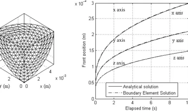
quarter domain meshed using 540 elements as shown in Figure 2. The step time is set at 10-2s. CPU time for the complete simulation is around one hour on Intel® Core™2 Duo CPU (2.26 GHz, 1.93 Go of RAM) using Matlab® environment. The computed flow fronts are in fair agreement with the analytical one as shown in Figure 3. At 10 s elapsed time, the deviations between the numerical and analytical flow fronts positions do not exceed 1%. Prolongating the simulation until 60 s gives deviations around 3%, due to the gradual mesh degeneration as the iterations go along. Figure 4 illustrates the flow front evolution during the filling stage, comparing the front shapes at t=0.5 s and t=10s.
Figure 2: Initial mesh domain Figure 3: Comparison with analytical solution
The initial mesh generation is performed on the equivalent isotropic domain. In order to assess the mesh effect on the numerical method, some simulations have been carried out meshing the physical domain. Deviations are all the more important that the permeability values are different. This is due to the transformation from Eq. 3 which stretches the mesh, degenerating elements before any calculation.
Flow front at t=0.5 s Flow front at t=10 s
Figure 4: Flow front computed at t=0.5 s and t=10 s x axis
y axis
Conclusion
The 3D radial front propagation is accurately simulated. The proposed technique is able to give a high accuracy of the front position, making it suitable for front tracking in permeability measurement [9]. It is a great advantage comparing to Volume Of Fluid techniques.
However, the proposed method is not directly applicable to complex shapes, because there is no contact algorithm implemented. In order to perform it, current works [10] focus on fixed grid approach, more suitable to handle contact (in particular merging and dividing fronts).
Future works will include hydro-mechanical couplings occurring during Liquid Composite Molding process, such as fibrous perform deformations.
Acknowledgments
This work was supported by DAHER-Socata and CRCC-Resource and Competencies Center for Composite Materials. The authors are especially grateful to M. Niquet for its assistance during this works.
References
[1] N.C. Correia, F. Robitaille, A.C. Long, C.D. Rudd, P. Simacek, S.G. Advani, Analysis of the vacuum infusion moulding process: I. Analytical formulation, Composites: part A 36 (2005). [2] M.-K. Um and W.I. Lee, A study on the Mold Filling Process in Resin Transfer Molding,
Polymer Engineering and Science, Vol. 31, No. 11 (Mid-June 1991).
[3] F.M. Schmidt, P. Lafleur, F. Berthet, P. Devos, Numerical Simulation of Resin Transfer Molding Using Linear Boundary Element Method. Polymer Composites. Vol. 20, No. 6, 725-732 (1999).
[4] S. Soukane, F. Trochu. Application of the level set method to the simulation of resin transfer molding. Composites Science and Technology 66, 1067-1080 (2006).
[5] H. Darcy, Les Fontaines Publiques de la Ville de Dijon. V. Dalmont, Paris, 1856 (in French). [6] K.L. Adams, W.B. Russel, L. Rebenfeld. Radial penetration of viscous liquid into a planar
anisotropic porous medium. International Journal Of Multiphase Flow, Vol. 14, No. 2 (1988). [7] C.A. Brebbia, J. Dominguez, Boundary Elements : an introductory course. 2nd ed.,
McGraw-Hill Company: Computational Mechanics Publications (1992).
[8] N. Pirc, F. Bugarin, F. Schmidt, M. Mongeau. BEM-based cooling optimization for 3D injection molding. International Journal for Simulation and Multidisciplinary Design Optimization, Vol. 2, No. 3 (2008).
[9] P.B., Nedanov, S.G. Advani. A method to determine 3D permeability of fibrous reinforcements. Journal of composite materials (2002).
[10] R. Gantois, A. Cantarel, G. Dusserre, J.-N. Félices, F. Schmidt. Numerical Simulation Of Resin Transfer Molding Using BEM and Level Set Method, 13th ESAFORM Conference on Material Forming, Proceedings (2010).