Understanding urban development types and drivers in Wallonia. A multi-density approach

Understanding urban development types and

drivers in Wallonia. A multi-density approach

Abstract. In this study, urban development process in the Walloon region

(Belgium) has been analysed. Two main aspects of development are quantitatively measured: the development type and the definition of the main drivers of the urbanisation process. Unlike most existing studies that consider the urban development as a binary process, this research considers the urban development as a continuous process, characterized by different levels of urban density. Eight urban classes are defined based on the Belgian cadastral data for years 2000 and 2010. A multinomial logistic regression model is employed to examine the main driving forces of the different densities. Sixteen drivers were selected, including accessibility, geo-physical features, policies and socio-economic factors. Finally, the changes from the non-urban to one of the urban density classes are detected and classified into different development types.

The results indicate that zoning status (political factor), slope, distance to roads, population densities and mean land price respectively have impact on the urbanization process whatever maybe the density. The results also show that the impact of these factors highly varies from one density to another.

Keywords: urban development; urban density; development type; driving

1 Introduction

Progress in urban development increases the consumption of natural resources and may eventually cause environmental impacts. Therefore, urbanization processes attract increasing attention (e.g. Batty, Xie and Sun, 1999; Asensio, 2000; Hallowell and Baran, 2013; Kryvobokov et al., 2015; Mustafa et al., 2015). Exiting models do usually not differentiate between high-density and low-density urban developments (e.g. Li, Zhou and Ouyang, 2013; Maimaitijiang et al., 2015). Yeh and Li (2002) argue that examining the development of different urban densities is an important factor in urban planning to help urban planners to set desirable urban density and forms according to different planning objectives. Mustafa et al. (2016) conclude that the assessment of urban flood damage is highly improved by using several urban densities instead of urban/non-urban classes.

This paper addresses the question of how to monitor and explain different forms of urbanization over time. To do that, this study explores and assesses urban development along seven urban-density classes against non-urban class in the Walloon region (southern part of Belgium) in terms of: (1) the main factors that steer the development and (2) the development type over time.

In the past two decades, substantial advances have been made in urban modelling studies through a wide range of analytic models to observe and/or predict urban patterns. The existing analytic models can be generally classified either as prescriptive or descriptive models. Prescriptive models aim at determining the optimum urban patterns that satisfy a set of goals, whereas descriptive models aim at the analysis and simulation of current and/or future expected patterns. In line with the aims of this study, we focus on descriptive models. Several descriptive modelling approaches have been developed to analyse urban patterns. Generally, the main approaches adopt cellular automata (e.g. Batty, Xie and Sun, 1999; Feng et al., 2011; Mustafa et al., 2014), agent‐based (e.g. Zhang et al., 2010; Augustijn-Beckers, Flacke and Retsios, 2011), urban-economic discrete-choice (e.g. Waddell, 2002; Kryvobokov et al., 2015), statistical models (e.g. Hu and Lo, 2007; Vermeiren et al., 2012; Li, Zhou and Ouyang, 2013), machine learning (e.g. Azari et al., 2016) and the integration of different models (e.g. Liu et al., 2014; Mustafa et al., 2015). A comprehensive review of a range of modelling approaches can be found in Briassoulis (2000), Verburg et al. (2004) and Brown et al. (2012). In this study, a statistical modelling approach is employed to track and analyse the development process. A multinomial logistic regression model (MLR) is selected to estimate the relationship between several urbanization driving factors and urban densities.

The expansion types of each urban density class can identify the future trend of each class. For instance, if a magnitude of new urban lands, related to a specific density class between two time-steps, is within existing urban cores, then the development behaviour of this class tends to be compacted. Authors defined three general development types (Hoffhine Wilson et al., 2003; Sun et al., 2013): (1) infill development, (2) edge-development and (3) outlying edge-development. In this study, the three types of development (figure 1) are measured for each density class.

Fig. 1. Urban development types

This paper is structured as follows. Section 2 gives an overview of potential urbanization drivers. Section 3 describes study area and presents the methodology and the data preparation process. Section 4 gives the detailed results and discusses the findings of this study, and finally the paper concludes with a brief remark and some policy-recommendations.

2 Potential driving forces

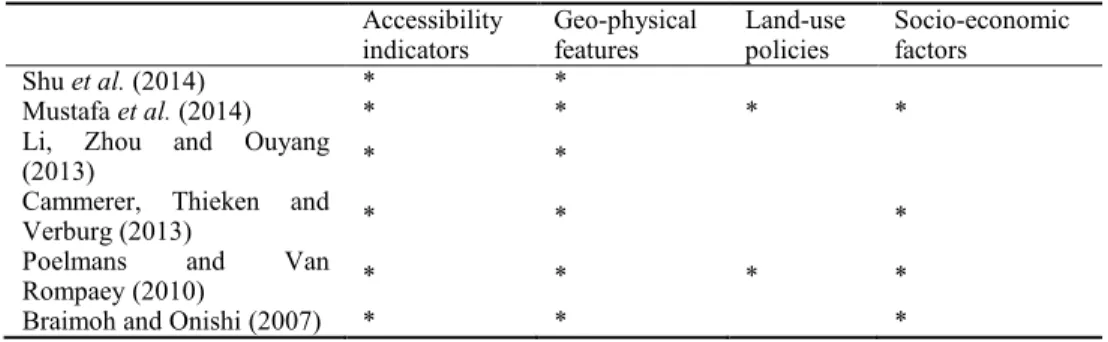
Although there is no universal driving forces for urban development, researchers have proposed various factors (table 1) which can be grouped into four main sets: (i) accessibility indicators, (ii) geo-physical features, (iii) land-use policies and (iv) socio-economic factors (table 1).

Table 1. Summary of the driving factors of urban development in the literature.

Accessibility

indicators Geo-physical features Land-use policies Socio-economic factors

Shu et al. (2014) * *

Mustafa et al. (2014) * * * *

Li, Zhou and Ouyang

(2013) * *

Cammerer, Thieken and

Verburg (2013) * * *

Poelmans and Van

Rompaey (2010) * * * *

Accessibility indicators are often included in urban development models by means of simple indicators, such as distance to cities, distance to the road network and distance to water bodies (Serneels and Lambin, 2001; QUAN et al., 2006; Braimoh and Onishi, 2007). In this study, we considered Euclidean distances to different roads categories and to the 11 Belgian cities with the largest population.

Geo-physical factors are commonly considered as major drivers of the spatial distribution and expansion of urban areas (Li, Zhou and Ouyang, 2013). There is often a relationship between development and a number of these factors, especially the topography of the study area (Cammerer, Thieken and Verburg, 2013; Li, Zhou and Ouyang, 2013). We considered elevation and slope as geo-physical factors in this study.

Zoning status is often considered as one of the potential urban development drivers. It has been classified as the most pervasive driver in USA (Brueckner, 2011). In the Walloon region, land allocation is controlled by several regulations including the regional development plan, referred to as "plan de secteur (PDS)". In this paper, we consider this zoning plan, which defines the legally authorized land-use type for all the territory.

This study also selects a number of socio-economic factors. Population is one of the most active drivers of development (Liu and Ma, 2011). In this respect, the evolution of net and gross population densities and number of households were considered. Economic development could also be considered as a driver of urban development; there is a relation between economic increase and urban development (Liu and Ma, 2011) and furthermore economic development has an important influence on people's location choices. In this respect, employment rate, richness level, housing and land prices are considered.

3 Methodology

3.1 Study area

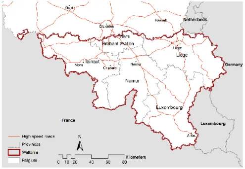
The Walloon region lies between latitudes 49°28' and 50°49'N and stretches between longitudes 2°50' and 6°28'E (figure 2). The Walloon region is the predominantly French-speaking region of Belgium. It has a territory of 16,844 km², corresponding to 55% of the Belgium territory. The population size in 2010 was equal to 3,498,384 inhabitants, representing a third of the entire Belgian population (Belgian Federal Government, 2015). Administratively, it comprises five provinces: Hainaut, Liège, Luxembourg, Namur, and Walloon Brabant. It has 20 administrative arrondissements and 262 municipalities. The geography of

the area goes from flat to hilly with altitude ranges from 0 to 693m above see-level.

The main metropolitan areas are Charleroi, Liège, Mons and Namur. They are all characterized by a historical city-centre around which the urban development was spread. Urban density greatly varies over the study area. The population is mainly concentrated on the main metropolitan centres. The rest of the territory is less densely inhabited. Consequently, several urban densities can be easily detected in the region and thus we can examine the sensitivity of different urbanization drivers to urban density.

Fig. 2. Study area

3.2 Multinomial logistic regression (MLR) model

Binomial logistic regression models are used whenever the dependent variable is binary which takes values 0 or 1. When a dependent variable has more than two categories then a multinomial logistic regression models can be used. The multinomial logistic regression models have two basic forms, ordinal and non-ordinal (often referred to simply as MLR). The ordinal one is employed whenever each category of dependent variable is assumed to have a meaningful sequential order. Parallel lines test is usually performed to evaluate this assumption. In this study, the significance of Chi-Square statistic of the parallel lines test is 0.000. Given that the assumption of the parallel lines is violated, and thus we have to adopt a non-ordinal alternative (MLR).

The MLR model is applied to investigate the contribution of the selected driving forces (independent variables, X) on the probability of urban development along the different density classes (dependent variables, Y). The MLR analysis yields coefficients for each driving force (X). These coefficients are then interpreted as weights in a formula that generates a map for each urban density class depicting the probability of each cell in the landscape to be converted into this class. If the Y variable is a categorical map with k classes, taking on values 0, 1,..., k-1 and X is a set of explanatory variables X1, X2,..., Xn then the logit for each non-reference

class k1,..., kn against the reference class k0 model is calculated through:

   









 is the natural logarithm of class kn against the reference

class k0, α is the intercept, βkn is the regression coefficients of class kn.

The probabilities P of each class can be calculated with the following formula: 1 1 0 log( ) log( ) log( ) log( ) log( ) 1 ( ) 1 ... ... ( ) 1 ... n n n k k k n k k P Y k e e e P Y k e e           (2)

The goodness-of-fit, in terms of predictive ability and the interpretability, of the MLR outcomes is evaluated using the McFadden pseudo R-square and the Relative Operating Characteristic (ROC) statistic respectively (Clark and Hosking, 1986; Braimoh and Onishi, 2007; Lin et al., 2014; Mustafa et al., 2014; Shu et al., 2014).

The McFadden pseudo R-square (MFR2) tries to mimic the R-squared statistic of linear regression models. An MFR2 of 1 indicates a perfect fit, while MFR2 of 0 indicates no relationship. It is calculated according to the following formula: 0 ln( ) 2 1 ln( ) m L MFR L   (3)

where Lm is the value of the likelihood function for the full model as fitted

with X and L0 is the value of the likelihood function if all β except α are 0.

The ROC statistic compares the probability map, produced by the MLR, to a map with the observed changes of urban cells for each class between two time-steps. It first divides the probability outcomes into percentile groups

from high to low probability and then calculates the proportion of true-positives and false-true-positives for a range of specified threshold values and relates them to each other in a graph. The ROC measures the area under the curve and its value should range between 0.5 (random fit) and 1 (perfect fit).

Prior to performing the MLR model, we have to consider three aspects that may exist among the model inputs that might potentially affect the regression results: disparity in units, autocorrelation and multicollinearity. Due to disparity in units and scale of the explanatory variables (table 4), the logit coefficients cannot be used directly to measure the relative contribution of each variable to the urban development process. Consequently, all continuous X were standardized before performing the MLR model. Categorical X were not standardized to keep the meaning of the dummy variable.

Spatial autocorrelation in one or more X will bias the results of the regression analysis. Autocorrelation is the propensity for cell value to be similar to surrounding cells. Moran's I statistic was processed to detect spatial autocorrelation for each X.It is given as:

1 1 2 1 ( )( ) _ ( ) n n ij i j i j n i ij i i j w x x M I n x w                     







where M_I is the Moran's I statistic for each X, n is the number of neighbour cells to be taken into account, w spatial weights and Xi/j cells

values at location i/j. The locations depend on the cell neighbours, considering shared-border neighbours (Xi) and possibly also diagonal

neighbours (Xj). We considered only Xj neighbours. Moran's I value ranges

between -1 and +1, where +1 means absolute autocorrelation and -1 none autocorrelation. To reduce the spatial autocorrelation, it is recommended to calibrate the model based on a structured or random sample from the whole dataset (Huang, Xie and Tay, 2010; Poelmans and Van Rompaey, 2010; Cammerer, Thieken and Verburg, 2013; Puertas, Henríquez and Meza, 2014; Rienow and Goetzke, 2015). Alternatively, an autologistic regression which considers an autocorrelative term in the regression model can be employed. A number of studied showed that the autologistic regression model outperformed the logistic models (e.g. Lin et al., 2011; Shafizadeh-Moghadam and Helbich, 2015). Contrary, some studies (e.g. Dormann, 2007) reported that the logistic regression model tends to outperform the autologistic regression model in terms of model parameters estimation. Comparing both modelling approaches (logistic vs autologistic) goes beyond the scope of this paper. Our model has been

calibrated through a data sampling approach, which is a common approach in land-use change modelling.

Multicollinearity represents a high degree of dependency among a number of X. It commonly occurs when a large number of X are introduced in a regression model. It is because some of X may relatively measure the same phenomena. Strong collinearities cause the erroneous estimation of parameters and further affect the MLR results (Lin et al., 2014). In this context, a number of procedures is proposed to detect multicollinearity among X such as tolerance value, variance inflation factor and Belsley diagnostics (Belsley, Kuh and Welsh, 1980; Judge et al., 1985; Belsley, 1991; Kennedy, 2003). We used Belsley diagnostics to detect multicollinearity. The outcomes of Belsley diagnostics are condition indices and variance-decomposition proportions for each X. A condition index greater than 30 represents strong multicollinearity (Kennedy, 2003). In that case, it is highly recommended to omit all X with variance-decomposition proportions exceeding the tolerance of 0.5 (Kennedy, 2003).

3.3 Dependent variables

The dependent variables are constituted by cells, whose status remains non-urban and whose status changed from non-urban to one of urban density classes between 2000 and 2010. The cadastral dataset (CAD) was used to develop the dependent variables map. CAD is a vector map representing buildings in two dimensions as polygons provided by the land registry administration of Belgium. Each building comes with different attributes, from which the construction date is the most important attribute for our study. Using the construction date, two urban land-use maps were developed for 2000 and 2010 years. The CAD vector data were rasterized at a very fine cell dimension (2×2m). Due to the time and computational resources constraints, the MLR model lasts for about 13 hours to manage 2×2m raster data, the rasterized cells were then aggregated to obtain 100×100m raster-grids. The cell size of 100×100m is one of the most common cell dimensions used in land-use change studies (e.g. Jiang et al., 2007; Poelmans and Van Rompaey, 2010; Sang et al., 2011; Munshi et al., 2014), which allows cross-comparisons with standard datasets like Corinne Land Cover. Each aggregated cell has a density value that represents the number of rasterized 2×2m cells. This value has been used to introduce the density in the aggregated CAD maps (100×100m raster-grid).

In order to avoid overestimation of urban lands, two measures were applied to the aggregated data: the minimum building density per cell (MBDC) and the minimum building density per neighbour (MBDN).

The average size of residential building in Belgium is about 10×10m (Tannier and Thomas, 2013). The MBDC has been defined as 25 rasterized cells (corresponding to an average-sized building).

A threshold of five dwellings per hectare, corresponding to 5×25 rasterized cells, was fixed for considering that a cell was urbanized. Neighbourhoods with such a density are indeed observable in the Walloon region. We then performed an analysis using different thresholds of MBDN using a search window of 3×3 cells for each MBDN cell less than 125 (5×25). These thresholds are 125, 250, 625, 1250 and 2500. Table 2 lists a comparison between (CORINE Land Cover) CLC data, CAD original aggregated data and different MBDN thresholds.

Table 2. Comparison of area (km²) between CLC, CAD_Org original aggregated CAD data,

MBDN_125, MBDN_250, MBDN_625, MBDN_1250 and MBDN_2500.

Year CLC CAD_Org MBDN1₂₅ MBDN ₂₅₀ MBDN ₆₂₅ MBDN ₁₂₅₀ MBDN ₂₅₀₀

2000 2506 3229 2599 2468 2093 1744 1579

2006 2513 - - - -

2010 - 3339 2716 2594 2230 1868 1693

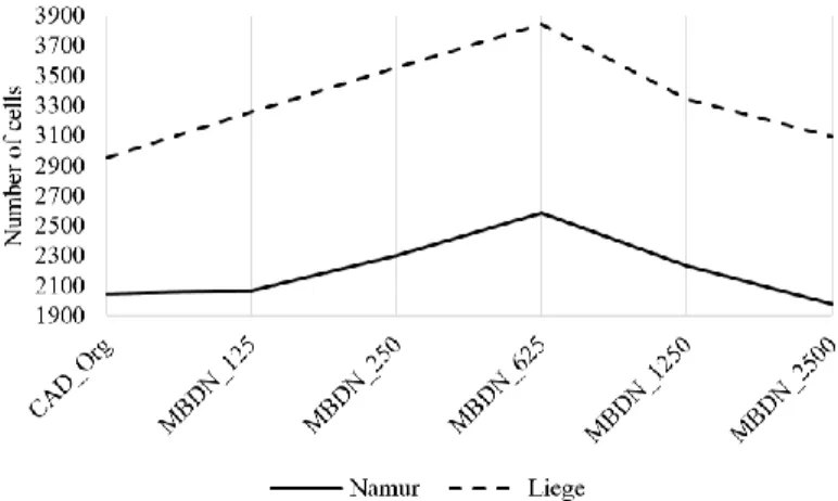
We assumed that the number of changed cells between two time-steps would increase until a specific value of MBDN and then start declining along with the increase of MBDN. Actually, those cells are under development at time-step 0 and reach the threshold of MBDN at time-step 1 are then considered as urban. If the MBDN threshold is very high, this condition will not be reached because this threshold exceeds the observed number of built cells at time-step 0 and 1. The number of changed cells calculated in two provinces of the Walloon region confirmed our assumption (figure 3). The result showed that the most appropriate threshold for the MBDN is 625.

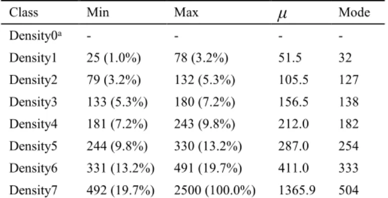
We performed different multinomial logistic regression (MLR) models for 4, 6, 8 and 10 urban densities quantile classes (including the non-urban class) and measured the goodness-of-fit in terms of misclassification rates. The misclassification rates equalled 24.23%, 23.60%, 22.70% and 26.07%, respectively. As a result, for the final MLR, we used eight urban classes, from Density0 (non-urban) to Density7 (highest urban-density), each class has almost the same number of cells except for Density0 (Figure 4). Table 3 lists the density range for each class.

Fig. 4. Urban density classes of 2010 (7 highest density, 1 lowest density)

Table 3. Urban classes density ranges in number of 2x2 pixels (% of 100x100 cell area)

covered by building footprints.

Class Min Max _μ Mode

Density0a _{- - - -} Density1 25 (1.0%) 78 (3.2%) 51.5 32 Density2 79 (3.2%) 132 (5.3%) 105.5 127 Density3 133 (5.3%) 180 (7.2%) 156.5 138 Density4 181 (7.2%) 243 (9.8%) 212.0 182 Density5 244 (9.8%) 330 (13.2%) 287.0 254 Density6 331 (13.2%) 491 (19.7%) 411.0 333 Density7 492 (19.7%) 2500 (100.0%) 1365.9 504

a _{Density0 represents all non-urban cells and affected cells by MBDC and MBDN procedures. μ:}

3.4 Independent variables

Statistical data related to the population volume, the number of households, the employment rate, the richness index (a comparison of the average income per capita in a given municipality with the average income per capita in Belgium) and the mean land/housing price were provided by the official Belgian statistics (Institut wallon de l’évaluation, de la prospective et de la statistique, 2011; Belgian Federal Government, 2013) and mapped with a resolution of 100×100m raster-grid at municipality level. Gross population density was calculated for each municipality as the number of inhabitants divided by the area of municipality in km², whereas net population density was calculated as the number of inhabitants divided by the area of built-up lands of the municipality in km².

The digital elevation model (DEM) provided by the Belgian National Geographic Institute was used to calculate elevation and slope in percentage for each cell.

Accessibility was measured by the Euclidean distance of a cell to four categories of roads and major Belgian cities. Roads categories of 2002 were provided by Navteq. Four categories of roads were introduced in the MLR (highways: high speed and volume controlled access roads, major_roads: quick travel between and through cities, secondary_roads: moderate speed travel within cities and local_roads: moderate speed travel between neighbourhoods). The Belgian cities with the largest population, a minimum population of 30,000, (Antwerp, Brussels, Wavre, Brugge, Gent, Charleroi, Mons, Liege, Hasselt, Arlon and Namur) were used to develop a map of distances to cities.

According to the zoning plan of the Walloon region, urban development is only allowed in those zones that are designated for residential, economic or leisure development. In other zones, such as agricultural and forest areas, urban development is not permitted, unless specific conditions are fulfilled. A zoning map was developed by discerning the zones where urban development is not permitted (code 0) and the zones that are designated for urban development (code 1). All maps were created as raster grids with a resolution of 100×100m (table 4). The spatial resolution is defined in function of the availability of data. The statistical data are available at municipality level, whereas other variables could be calculated at cell level. The combination of data at different resolutions is common in land-use studies (e.g. Cammerer, Thieken and Verburg, 2013; Roy Chowdhury and Maithani, 2014).

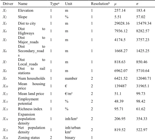
Table 4. List of the selected drivers of urban development.

Driver Name Typea _{Unit Resolution}b _{μ σ}

X1 Elevation 1 m 1 257.14 183.4 X2 Slope 1 % 1 5.51 57.02 X3 Dist to city 1 m 1 29028.16 15479.34 X4 Dist _Highways to 1 m 1 7936.12 8282.57 X5 Dist _{Major_roads} to 1 m 1 4174.5 3757.23 X6 Dist to Secondary_road s 1 m 1 1668.27 1425.25 X7 Dist _{Local_roads} to 1 m 1 818.63 850.46

X8 Dist _stations to rail 1 m 1 6962.07 5710.64

X9 Num households 1 number 2 6421.52 12040.71

X10 Mean housing _price 1 € 2 139487 31965.1

X11 Mean land price 1 €/m² 2 51.1 99.73

X12 Employment _potential 1 % 2 48.39 98.42 X13 Richness index 1 % 2 95.71 61.62 X14 Expansion population density 1 inh/km² 2 206.95 354.33

X15 Net population _density 1 inh/urban _km² 2 819.52 522.97

X16 Zoning status 2 binary 1

a _{1. Continuous, 2. Categorical.} b _{1. Cell level, 2. Municipality level. μ: mean. σ: standard deviation}

3.5 Identification of urban development types

Each type of urban development leads to different planning and environmental consequences. Thus, identifying the types of development over time is essential for monitoring and alleviating the consequences of the urbanization process (Luck and Wu, 2002). In this context, three types of development are measured for each density class.

The first type of development is infill. In this type of development, the non-urban cells which are completely surrounded by urban cells, are converted to cells corresponding to one of the density classes. Infill development usually occupies vacant land, where public facilities such as sewer, water, and roads already exist (Hoffhine Wilson et al., 2003). The second type of development is edge-development, where non-urban cells, which adjoin existing urban cells, are converted to one of the density classes. This type represents an expansion of the existing urban patch and has been called urban fringe development (Wasserman, 2000; Hoffhine Wilson et al., 2003)

The final type of urban development is outlying, in which non-urban cells are being converted to one of the density classes beyond existing developed areas.

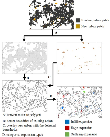
In order to identify expansion type, the raster maps of existing urban patches associated with newly developed urban patches were firstly converted to vector maps. Following the conversion steps, the boundaries of each existing urban patch were detected.

The vector maps (map for each density class) of newly developed urban patches were overlaid with the boundaries of each existing urban patch. Using Select By Location function in ArcGIS, if the newly developed urban patch was within the boundaries of existing urban patch, the patch was categorized as infill development. If the newly developed urban patch touches the boundary of existing urban patches, the patch was categorized as edge-development. All other newly urban patches were then classified as outlying development (figure 5).

4 Results and discussions

The urban area in 2000 in the Walloon region was 2093 km², accounting for 12.4% of the total area, and in 2010, the urban area increased to 2230 km², accounting for 13.2% of the total area. The rate of increase varies based on density (table 3): 36.6% (50.3 km²) for Density1, 25.3% (34.8 km²) for Density2, 16.6% (22.9 km²) for Density3, 7.6% (10.5 km²) for Density4, 5.2% (7.1 km²) for Density5, 3.9% (5.3 km²) for Density6 and finally 4.9% (6.7 km²) for Density7.

As regard with the MLR model, all explanatory variables (X) have strong degree of spatial autocorrelation with Moran's I value between 0.746 for zoning and 0.999 for distance to cities. To reduce the spatial autocorrelation, a random sample of 15,675 cells, around 1.15% of the study area, distributed throughout the study area was used in the MLR model. All X show low degree of multicollinearity with condition indices between 1 and 9.15 for all X maps and 1 to 9.86 for the selected samples. Thus, all X are introduced in the MLR model.

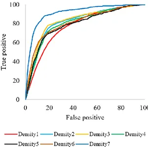
The goodness-of-fit of the MLR model in terms of predictive ability is evaluated using McFadden pseudo R-square and it equals 0.244. Clark and Hosking (1986) suggested that a McFadden pseudo R-square value greater than 0.2 can be considered as a good fit. The MLR reveals a very good correspondence with ROC values (figure 6): 0.775, 0.819, 0.829, 0.805, 0.793, 0.813 and 0.914 for classes 1, 2, 3, 4, 5, 6 and 7 respectively. In general, ROC values higher than 0.7 can be considered as a reasonable fit (Jr and Lemeshow, 2004; Poelmans, 2010; Cammerer, Thieken and Verburg, 2013). This indicates that the MLR performs well and the MLR’s outcomes could effectively interpret the process of urban development in the Walloon region.

Table 5 gives the results of the MLR model. To relatively measure the contribution of each X to the urban development process, the Odds Ratio (OR), which equals exp(β), is calculated for each X. An OR greater than 1 (coefficients greater than 0) indicates a positive effect, i.e. the probability of development increases by increasing the OR of the variable, whereas an

OR less than 1 (coefficients less than 0) indicates a negative effect, i.e. the

probability of urban development decreases by increasing the OR of the variable. An OR of 1 (coefficients of 0) indicates the absence of a significant contribution to development process (Braimoh and Onishi, 2007).

The interpretation of the parameters of the MLR model is most tangible by considering the interpretation in terms of multiplicative effects on the odds. Take as an example the parameter representing the effect of elevation on Density7 expansion. This parameter equals 0.110. A one unit increase would in elevation would imply that we have to multiply the odds

by exp(0.110) = 1.117. Similarly, a five unit increase would imply that the odds have to be multiplied by exp(5x0.110) = 1.7.

Generally, the impact of different drivers varies with different densities. These drivers can be grouped into common drivers with impacts on different urban classes and special drivers with impacts on individual classes. The likelihood of urban development is notably influenced by policies (zoning status). Zoning status has the strongest impact on urban developments of all densities. Slope, distance to local_roads, distance to secondary_roads, net/gross population densities and mean land price respectively also demonstrate an impact on all density classes, but far less important than zoning status.

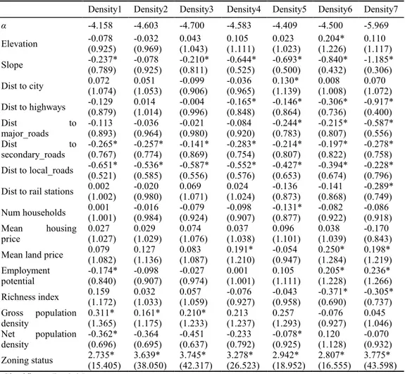
Table 5. The coefficients (β) of MLR model and (OR value). Density0 is the reference class.

Density1 Density2 Density3 Density4 Density5 Density6 Density7

α -4.158 -4.603 -4.700 -4.583 -4.409 -4.500 -5.969 Elevation -0.078 _(0.925) -0.032 _(0.969) 0.043 _(1.043) 0.105 _(1.111) 0.023 _(1.023) 0.204* _(1.226) 0.110 _(1.117) Slope -0.237* _(0.789) -0.078 _(0.925) -0.210* _(0.811) -0.644* _(0.525) -0.693* _(0.500) -0.840* _(0.432) -1.185* _(0.306) Dist to city 0.072 _(1.074) 0.051 _(1.053) -0.099 _(0.906) -0.036 _(0.965) 0.130* _(1.139) 0.008 _(1.008) 0.070 _(1.072) Dist to highways -0.129 _(0.879) 0.014 _(1.014) -0.004 _(0.996) -0.165* _(0.848) -0.146* _(0.864) -0.306* _(0.736) -0.917* _(0.400) Dist to major_roads -0.113 (0.893) -0.036 (0.964) -0.021 (0.980) -0.084 (0.920) -0.244* (0.783) -0.215* (0.807) -0.587* (0.556) Dist to secondary_roads -0.265* (0.767) -0.257* (0.774) -0.141* (0.869) -0.283* (0.754) -0.214* (0.807) -0.197* (0.822) -0.278* (0.758) Dist to local_roads -0.651* _(0.521) -0.536* _(0.585) -0.587* _(0.556) -0.552* _(0.576) -0.427* _(0.653) -0.394* _(0.674) -0.228* _(0.796) Dist to rail stations 0.002 _(1.002) -0.020 _(0.980) 0.069 _(1.071) 0.024 _(1.024) -0.136 _(0.873) -0.141 _(0.868) -0.289* _(0.749) Num households 0.001 _(1.001) -0.016 _(0.984) -0.079 _(0.924) -0.098 _(0.907) -0.131* _(0.877) -0.082 _(0.922) -0.086 _(0.918) Mean housing

price 0.027 (1.027) 0.029 (1.029) 0.074 (1.076) 0.037 (1.038) 0.096 (1.101) 0.038 (1.039) -0.170 (0.843) Mean land price 0.079 _(1.082) 0.127 _(1.136) 0.083 _(1.087) 0.191* _(1.210) -0.054 _(0.947) 0.250* _(1.284) 0.198* _(1.219) Employment potential -0.174* (0.840) -0.098 (0.907) -0.027 (0.974) 0.001 (1.001) 0.105 (1.111) 0.205* (1.228) 0.236* (1.266) Richness index 0.159 _(1.172) 0.032 _(1.033) 0.057 _(1.059) -0.076 _(0.927) -0.043 _(0.958) -0.371* _(0.690) -0.305* _(0.737) Gross population density 0.311* (1.365) 0.161* (1.175) 0.210* (1.233) 0.213 (1.237) 0.257 (1.293) -0.076 (0.927) 0.045 (1.046) Net population density -0.362* (0.696) -0.364 (0.695) -0.451 (0.637) -0.233 (0.792) -0.078* (0.925) 0.120 (1.128) -0.070 (0.932) Zoning status 2.735* _(15.405) 3.639* _(38.050) 3.745* _(42.317) 3.278* _(26.523) 2.942* _(18.952) 2.807* _(16.555) 3.775* _(43.598) * Significant P≤ 0.05

Fig. 6. ROC curves of different urban classes

The impact of distance to local_roads, namely intra-urban or inter-villages roads, is generally decreasing with built-up densities. Distances to highways and major_roads have a noticeable impact on the expansion of high density projects (Density7) with OR of 0.40 and 0.56 respectively. It should be stressed that a number of urban cores are directly accessible via high-speed roads in the Walloon region. Employment potential has a significant attraction impact on Density7. It is generally increasing with density, which is what can be expected. The richness index and elevation have moderate impacts on urban Density6. Distance to rail stations has a moderate positive influence on urban Density7. Still this influence is much lower than the proximity of high-speed roads, suggesting that urban areas located nearby train stations are not yet sufficiently attractive for new dense developments. This should be a major concern for urban policy makers. Mean housing price represents a low influence on urban development. This influence is negative for high density developments, which is another source of concern given the shortage of available housing, especially apartments, in areas characterized by a strong pressure on the real estate market.

OR values for zoning show that policy has a very strong impact on the highest density developments (Density7). Those high density developments will most naturally be developed in areas where the legally-binding plan allows such developments, in order to minimize the administrative and financial risks of such operations. Zoning status impact is taken a downward trend with classes 4, 5 and 6 respectively. We consider those classes as suburbs. Quite understandably that urban

developments in suburbs do not strictly follow policies. The zoning impact on Density1 is very low compared to other classes. This class can be considered as remote developments which can sometimes deviate from existing zoning plans especially in agricultural zones. Land-use policies also show a noticeable impact on classes 2 and 3. We considered those both classes as low density developments in rural areas. It is not surprising that new developments are mainly directed to urbanisable zones, where there is an excess supply of such land. The MLR findings are in line with the results reported in a number of other studies. Poelmans and Van Rompaey (2010) examined the relation between urban development in norther Belgium and slope, distance to different roads, major cities, employment potential and zoning status using logistic regression. They concluded that zoning status, slope, distance to roads are the major determinants of the spatial pattern of urban development. Hu and Lo (2007) used logistic regression to identify the forces that have driven the urban growth in Atlanta. They reported that population density and distance to roads were found to affect urbanization process.

General speaking, urban development patterns can be considered as an oscillation between phases of diffusion and coalescence over time (Winsborough, 1962; Yu and Ng, 2007; Shi et al., 2012). Diffusion is considered as a dispersion of urban patches, while coalescence is the fusion of urban patches into a limited number of patches (Dietzel et al., 2005; Shi et al., 2012). Infill and edge developments are forms of coalescence, whereas outlying developments represent diffusion (Xu et

al., 2007; Shi et al., 2012). The proportion of infill and edge urban

developments is about 92% of the total newly developed urban lands, which indicates that the urban development between 2000 and 2010 was obviously in the form of coalescence.

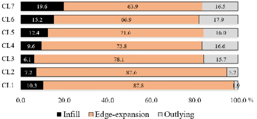
The edge-development was the dominant type of all urban classes’ expansion during the study period, occupying approximately 83% of the total newly developed urban lands (Figure 7). This implies that the urbanization process between 2000 and 2010 were prominently expanded in the urban fringe spaces.

Fig. 7. The area proportion (%) of each urban development type in 2000–2010

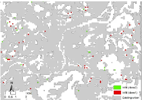
The result shows a gradual downward trend in the infill expansion type from Density7 till Density2 and then shows an upward trend. Most of infill newly urban patches of classes 1 and 2 are within major urban cores (Figure 8). Those patches might be under urban development at the current time and will be intensified in the future. The infill expansion type of Density7 is greater than other urban classes with the implication of compact urban growth near existing urban cores. In addition, the degree of outlying expansion of Density7 indicates that high-density expansion can also be found further from urban cores. Further analysis is still required to see whether the new discontinuous developments were followed by later efficient infill based on expansion patterns for different time periods. Due to shortages of available urban space and the high cost of construction in existing urban cores, investments in suburbs have become economically attractive especially for individuals. That can explain the higher values of the outlying expansion of density classes 7, 6, 5, 4 and 3.

Fig. 8. The area proportion (%) of each urban development type in 2000–2010

5 Conclusions

In this study, we presented a comprehensive analysis of recent urbanization process in the Walloon region (Belgium) between 2000 and 2010. A set of procedures were done to measure development types and the main drivers of the urbanization process. This research considered urban development as a continuum. It can be seen that the examination of different urban densities expansion help with better understanding of urbanization process and can be utilized by urban planners to generate development scenarios according to different density strategies.

An examination of the driving forces of urban development process in the Walloon region was required to help with improving land-use efficiency and minimizing destruction to the regional ecosystem. A multinomial logistic regression model (MLR) was employed to relatively measure the impact of different drivers on the probability of development. Sixteen drivers were selected from four sets of driving forces including geo-physical features, land-use policies, socio-economic and accessibility. The MLR model can include biophysical factors as well as socio-economic factors. The model’s ability to include as many socio-socio-economic factors as necessary allows us to better understand human interactions with urban systems. The MLR models can model any state. In the case of urban to non-urban, the modeller should select the urban class as a

reference class. The MLR also requires less demand of computation resources for calibration. Despite these strengths, the MLR models suffer some limitations. Firstly, it assumes that the occurrence probability is linearly and additively related to the controlling factors on a logistic scale (Cheng and Masser, 2003). If this assumption cannot be satisfied, the performance may degrade. Secondly, unlike other urbanization modelling approaches such as cellular automata or agent-based, the MLR models are not temporally explicit. In other words, it can indicate the location of a specific urban development, but cannot indicate when the development will take place.

Three types of urban development were detected: (1) infill development, (2) edge-expansion and (3) outlying expansion. The analysis indicated that the development between 2000 and 2010 was mainly of infill and edge developments, which reveals that the Walloon region experienced more compacted urbanization pattern. This result is consistent with a number of studies that refer to urban development have mostly concentrated in developed urban cores (e.g. Schneider and Woodcock, 2008; Petrov, Lavalle and Kasanko, 2009; Banzhaf and Lavery, 2010).

The results suggest that urban development in the Walloon region is remarkably influenced by land-use policies. Therefore, a tighter control of urban development through legislative measures would improve land-use efficiency. Our findings highlighted that the impact of different drivers varies along with urban density. This is especially the case for the land-use policies, whose effects are much more significant for smaller densities than for higher ones, with exception for the urban cores. Our approach can predict future land consumption in accommodating a specific number of dwellings along various levels of densities, which is critically important for policy makers to restrict urban sprawl.

References

Asensio, J. (2000) ‘The success story of Spanish suburban railways: determinants of demand and policy implications’, Transport Policy, 7(4), pp. 295–302. doi: 10.1016/S0967-070X(00)00030-5. Augustijn-Beckers, E.-W., Flacke, J. and Retsios, B. (2011) ‘Simulating informal settlement growth in Dar es Salaam, Tanzania: An agent-based housing model’, Computers, Environment and

Urban Systems, 35(2), pp. 93–103. doi: 10.1016/j.compenvurbsys.2011.01.001.

Azari, M., Tayyebi, A., Helbich, M. and Reveshty, M. A. (2016) ‘Integrating cellular automata, artificial neural network, and fuzzy set theory to simulate threatened orchards: application to Maragheh, Iran’, GIScience & Remote Sensing, 53(2), pp. 183–205. doi:

Banzhaf, H. S. and Lavery, N. (2010) ‘Can the land tax help curb urban sprawl? Evidence from growth patterns in Pennsylvania’, Journal of Urban Economics, 67(2), pp. 169–179. doi: 10.1016/j.jue.2009.08.005.

Batty, M., Xie, Y. and Sun, Z. (1999) ‘Modeling urban dynamics through GIS-based cellular automata’, Computers, Environment and Urban Systems, 23(3), pp. 205–233. doi: 10.1016/S0198-9715(99)00015-0.

Belgian Federal Government (2013) Statistics Belgium, Statistics Belgium. Available at: http://statbel.fgov.be/fr/statistiques/chiffres/ (Accessed: 29 April 2014).

Belgian Federal Government (2015) Population, Statistics Belgium. Available at: http://statbel.fgov.be/fr/modules/publications/statistiques/population/population_-_chiffres_population_1990-2010.jsp (Accessed: 19 April 2015).

Belsley, D. A. (1991) Conditioning diagnostics. Wiley Online Library. Available at:

http://onlinelibrary.wiley.com/doi/10.1002/0471667196.ess0275.pub2/full (Accessed: 21 March 2015).

Belsley, D. A., Kuh, E. and Welsh, R. E. (1980) Regression Diagnostics. John Wiley and Sons, New York.

Braimoh, A. K. and Onishi, T. (2007) ‘Spatial determinants of urban land use change in Lagos, Nigeria’, Land Use Policy, 24(2), pp. 502–515. doi: 10.1016/j.landusepol.2006.09.001. Briassoulis, H. (2000) Analysis of Land Use Change: Theoretical and Modeling Approaches. Wholbk. Regional Research Institute, West Virginia University. Available at:

http://econpapers.repec.org/bookchap/rriwholbk/17.htm (Accessed: 9 October 2016).

Brown, D. G., Walker, R., Manson, S. and Seto, K. (2012) ‘Modeling Land Use and Land Cover Change’, in Gutman, D. G., Janetos, A. C., Justice, C. O., Moran, D. E. F., Mustard, J. F., Rindfuss, R. R., Skole, D., II, B. L. T., and Cochrane, M. A. (eds) Land Change Science. Springer

Netherlands (Remote Sensing and Digital Image Processing, 6), pp. 395–409. Available at: http://link.springer.com/chapter/10.1007/978-1-4020-2562-4_23 (Accessed: 9 October 2016). Brueckner, J. K. (2011) Lectures on Urban Economics. MIT Press.

Cammerer, H., Thieken, A. H. and Verburg, P. H. (2013) ‘Spatio-temporal dynamics in the flood exposure due to land use changes in the Alpine Lech Valley in Tyrol (Austria)’, Natural Hazards, 68(3), pp. 1243–1270. doi: 10.1007/s11069-012-0280-8.

Cheng, J. and Masser, I. (2003) ‘Urban growth pattern modeling: a case study of Wuhan city, PR China’, Landscape and Urban Planning, 62(4), pp. 199–217. doi: 10.1016/S0169-2046(02)00150-0.

Clark, W. A. V. and Hosking, P. L. (1986) Statistical Methods for Geographers. 1 edition. New York: Wiley.

Dietzel, C., Oguz, H., Hemphill, J. J., Clarke, K. C. and Gazulis, N. (2005) ‘Diffusion and Coalescence of the Houston Metropolitan Area: Evidence Supporting a New Urban Theory’,

Environment and Planning B: Planning and Design, 32(2), pp. 231–246. doi: 10.1068/b31148.

Dormann, C. F. (2007) ‘Assessing the validity of autologistic regression’, Ecological Modelling, 207(2–4), pp. 234–242. doi: 10.1016/j.ecolmodel.2007.05.002.

Feng, Y., Liu, Y., Tong, X., Liu, M. and Deng, S. (2011) ‘Modeling dynamic urban growth using cellular automata and particle swarm optimization rules’, Landscape and Urban Planning, 102(3), pp. 188–196. doi: 10.1016/j.landurbplan.2011.04.004.

Hallowell, G. D. and Baran, P. K. (2013) ‘Suburban change: A time series approach to measuring form and spatial configuration’, The Journal of Space Syntax, 4(1), pp. 74–91.

Hoffhine Wilson, E., Hurd, J. D., Civco, D. L., Prisloe, M. P. and Arnold, C. (2003) ‘Development of a geospatial model to quantify, describe and map urban growth’, Remote Sensing of

Environment. (Urban Remote Sensing), 86(3), pp. 275–285. doi: 10.1016/S0034-4257(03)00074-9.

Hu, Z. and Lo, C. P. (2007) ‘Modeling urban growth in Atlanta using logistic regression’,

Computers, Environment and Urban Systems, 31(6), pp. 667–688. doi:

10.1016/j.compenvurbsys.2006.11.001.

Huang, B., Xie, C. and Tay, R. (2010) ‘Support vector machines for urban growth modeling’,

GeoInformatica, 14(1), pp. 83–99. doi: 10.1007/s10707-009-0077-4.

Institut wallon de l’évaluation, de la prospective et de la statistique (2011) Statistiques, IWEPS. Available at: http://www.iweps.be/themes-page (Accessed: 12 May 2014).

Jiang, F., Liu, S., Yuan, H. and Zhang, Q. (2007) ‘Measuring urban sprawl in Beijing with geo-spatial indices’, Journal of Geographical Sciences, 17(4), pp. 469–478. doi: 10.1007/s11442-007-0469-z.

Jr, D. W. H. and Lemeshow, S. (2004) Applied Logistic Regression. John Wiley & Sons. Judge, G. G., Griffiths, W. E., Hill, R. C., Lütkepohl, H. and Lee, T.-C. (1985) The Theory and

Practice of Econometrics. 2 edition. New York: Wiley.

Kennedy, P. (2003) A Guide to Econometrics. MIT Press.

Kryvobokov, M., Mercier, A., Bonnafous, A. and Bouf, D. (2015) ‘Urban simulation with alternative road pricing scenarios’, Case Studies on Transport Policy, 3(2), pp. 196–205. doi: 10.1016/j.cstp.2015.02.001.

Li, X., Zhou, W. and Ouyang, Z. (2013) ‘Forty years of urban expansion in Beijing: What is the relative importance of physical, socioeconomic, and neighborhood factors?’, Applied Geography, 38, pp. 1–10. doi: 10.1016/j.apgeog.2012.11.004.

Lin, Y., Deng, X., Li, X. and Ma, E. (2014) ‘Comparison of multinomial logistic regression and logistic regression: which is more efficient in allocating land use?’, Frontiers of Earth Science, pp. 1–12. doi: 10.1007/s11707-014-0426-y.

Lin, Y.-P., Chu, H.-J., Wu, C.-F. and Verburg, P. H. (2011) ‘Predictive ability of logistic regression, auto-logistic regression and neural network models in empirical land-use change modeling – a case study’, International Journal of Geographical Information Science, 25(1), pp. 65–87. doi: 10.1080/13658811003752332.

Liu, C. and Ma, X. (2011) ‘Analysis to driving forces of land use change in Lu’an mining area’,

Transactions of Nonferrous Metals Society of China, 21, Supplement 3, pp. s727–s732. doi:

Liu, X., Ma, L., Li, X., Ai, B., Li, S. and He, Z. (2014) ‘Simulating urban growth by integrating landscape expansion index (LEI) and cellular automata’, International Journal of Geographical

Information Science, 28(1), pp. 148–163. doi: 10.1080/13658816.2013.831097.

Luck, M. and Wu, J. (2002) ‘A gradient analysis of urban landscape pattern: a case study from the Phoenix metropolitan region, Arizona, USA’, Landscape Ecology, 17(4), pp. 327–339. doi: 10.1023/A:1020512723753.

Maimaitijiang, M., Ghulam, A., Sandoval, J. S. O. and Maimaitiyiming, M. (2015) ‘Drivers of land cover and land use changes in St. Louis metropolitan area over the past 40 years characterized by remote sensing and census population data’, International Journal of Applied Earth Observation

and Geoinformation, 35, Part B, pp. 161–174. doi: 10.1016/j.jag.2014.08.020.

Munshi, T., Zuidgeest, M., Brussel, M. and van Maarseveen, M. (2014) ‘Logistic regression and cellular automata-based modelling of retail, commercial and residential development in the city of Ahmedabad, India’, Cities, 39, pp. 68–86. doi: 10.1016/j.cities.2014.02.007.

Mustafa, A., Bruwier, M., Teller, J., Archambeau, P., Erpicum, S., Pirotton, M. and Dewals, B. (2016) ‘Impacts of urban expansion on future flood damage: A case study in the River Meuse basin, Belgium’, in Sustainable Hydraulics in the Era of Global Change. Taylor & Francis Group. Available at: http://orbi.ulg.ac.be/handle/2268/200745 (Accessed: 22 August 2016).

Mustafa, A., Saadi, I., Cools, M. and Teller, J. (2014) ‘Measuring the Effect of Stochastic Perturbation Component in Cellular Automata Urban Growth Model’, Procedia Environmental

Sciences. (12th International Conference on Design and Decision Support Systems in Architecture

and Urban Planning, DDSS 2014), 22, pp. 156–168. doi: 10.1016/j.proenv.2014.11.016. Mustafa, A., Saadi, I., Cools, M. and Teller, J. (2015) ‘Modelling Uncertainties in Long-Term Predictions of Urban Growth: A Coupled Cellular Automata and Agent-Based Approach’,

Proceedings of CUPUM 2015, p. 18.

Petrov, L. O., Lavalle, C. and Kasanko, M. (2009) ‘Urban land use scenarios for a tourist region in Europe: Applying the MOLAND model to Algarve, Portugal’, Landscape and Urban Planning, 92(1), pp. 10–23. doi: 10.1016/j.landurbplan.2009.01.011.

Poelmans, L. (2010) Modelling urban expansion and its hydrological impacts. Unpublished PhD dissertation. Katholieke Universiteit Leuven.

Poelmans, L. and Van Rompaey, A. (2010) ‘Complexity and performance of urban expansion models’, Computers, Environment and Urban Systems, 34(1), pp. 17–27. doi:

10.1016/j.compenvurbsys.2009.06.001.

Puertas, O. L., Henríquez, C. and Meza, F. J. (2014) ‘Assessing spatial dynamics of urban growth using an integrated land use model. Application in Santiago Metropolitan Area, 2010–2045’, Land

Use Policy, 38, pp. 415–425. doi: 10.1016/j.landusepol.2013.11.024.

QUAN, B., CHEN, J.-F., QIU, H.-L., RÖMKENS, M. J. M., YANG, X.-Q., JIANG, S.-F. and LI, B.-C. (2006) ‘Spatial-Temporal Pattern and Driving Forces of Land Use Changes in Xiamen’,

Pedosphere, 16(4), pp. 477–488. doi: 10.1016/S1002-0160(06)60078-7.

Rienow, A. and Goetzke, R. (2015) ‘Supporting SLEUTH – Enhancing a cellular automaton with support vector machines for urban growth modeling’, Computers, Environment and Urban Systems, 49, pp. 66–81. doi: 10.1016/j.compenvurbsys.2014.05.001.

Roy Chowdhury, P. K. and Maithani, S. (2014) ‘Modelling urban growth in the Indo-Gangetic plain using nighttime OLS data and cellular automata’, International Journal of Applied Earth

Observation and Geoinformation, 33, pp. 155–165. doi: 10.1016/j.jag.2014.04.009.

Sang, L., Zhang, C., Yang, J., Zhu, D. and Yun, W. (2011) ‘Simulation of land use spatial pattern of towns and villages based on CA–Markov model’, Mathematical and Computer Modelling. (Mathematical and Computer Modeling in agriculture (CCTA 2010)), 54(3–4), pp. 938–943. doi: 10.1016/j.mcm.2010.11.019.

Schneider, A. and Woodcock, C. E. (2008) ‘Compact, Dispersed, Fragmented, Extensive? A Comparison of Urban Growth in Twenty-five Global Cities using Remotely Sensed Data, Pattern Metrics and Census Information’, Urban Studies, 45(3), pp. 659–692. doi:

10.1177/0042098007087340.

Serneels, S. and Lambin, E. F. (2001) ‘Proximate causes of land-use change in Narok District, Kenya: a spatial statistical model’, Agriculture, Ecosystems & Environment, 85(1–3), pp. 65–81. doi: 10.1016/S0167-8809(01)00188-8.

Shafizadeh-Moghadam, H. and Helbich, M. (2015) ‘Spatiotemporal variability of urban growth factors: A global and local perspective on the megacity of Mumbai’, International Journal of

Applied Earth Observation and Geoinformation, 35, Part B, pp. 187–198. doi:

10.1016/j.jag.2014.08.013.

Shi, Y., Sun, X., Zhu, X., Li, Y. and Mei, L. (2012) ‘Characterizing growth types and analyzing growth density distribution in response to urban growth patterns in peri-urban areas of

Lianyungang City’, Landscape and Urban Planning, 105(4), pp. 425–433. doi: 10.1016/j.landurbplan.2012.01.017.

Shu, B., Zhang, H., Li, Y., Qu, Y. and Chen, L. (2014) ‘Spatiotemporal variation analysis of driving forces of urban land spatial expansion using logistic regression: A case study of port towns in Taicang City, China’, Habitat International, 43, pp. 181–190. doi:

10.1016/j.habitatint.2014.02.004.

Sun, C., Wu, Z., Lv, Z., Yao, N. and Wei, J. (2013) ‘Quantifying different types of urban growth and the change dynamic in Guangzhou using multi-temporal remote sensing data’, International

Journal of Applied Earth Observation and Geoinformation, 21, pp. 409–417. doi:

10.1016/j.jag.2011.12.012.

Tannier, C. and Thomas, I. (2013) ‘Defining and characterizing urban boundaries: A fractal analysis of theoretical cities and Belgian cities’, Computers, Environment and Urban Systems, 41, pp. 234–248. doi: 10.1016/j.compenvurbsys.2013.07.003.

Verburg, P. H., Schot, P. P., Dijst, M. J. and Veldkamp, A. (2004) ‘Land use change modelling: current practice and research priorities’, GeoJournal, 61(4), pp. 309–324. doi: 10.1007/s10708-004-4946-y.

Vermeiren, K., Van Rompaey, A., Loopmans, M., Serwajja, E. and Mukwaya, P. (2012) ‘Urban growth of Kampala, Uganda: Pattern analysis and scenario development’, Landscape and Urban

Planning, 106(2), pp. 199–206. doi: 10.1016/j.landurbplan.2012.03.006.

Waddell, P. (2002) ‘UrbanSim: Modeling Urban Development for Land Use, Transportation, and Environmental Planning’, Journal of the American Planning Association, 68(3), pp. 297–314. doi: 10.1080/01944360208976274.

Winsborough, H. H. (1962) ‘City Growth and City Structure†’, Journal of Regional Science, 4(2), pp. 35–49. doi: 10.1111/j.1467-9787.1962.tb00903.x.

Xu, C., Liu, M., Zhang, C., An, S., Yu, W. and Chen, J. M. (2007) ‘The spatiotemporal dynamics of rapid urban growth in the Nanjing metropolitan region of China’, Landscape Ecology, 22(6), pp. 925–937. doi: 10.1007/s10980-007-9079-5.

Yeh, A. G.-O. and Li, X. (2002) ‘A Cellular Automata Model to Simulate Development Density for Urban Planning’, Environment and Planning B: Planning and Design, 29(3), pp. 431–450. doi: 10.1068/b1288.

Yu, X. J. and Ng, C. N. (2007) ‘Spatial and temporal dynamics of urban sprawl along two urban– rural transects: A case study of Guangzhou, China’, Landscape and Urban Planning, 79(1), pp. 96– 109. doi: 10.1016/j.landurbplan.2006.03.008.

Zhang, H., Zeng, Y., Bian, L. and Yu, X. (2010) ‘Modelling urban expansion using a multi agent-based model in the city of Changsha’, Journal of Geographical Sciences, 20(4), pp. 540–556. doi: 10.1007/s11442-010-0540-z.