Forecasting the CATS benchmark with the Double Vector Quantization method

HAL Id: hal-00134938

https://hal.archives-ouvertes.fr/hal-00134938

HAL is a multi-disciplinary open access archive for the deposit and dissemination of sci-entific research documents, whether they are pub-lished or not. The documents may come from

L’archive ouverte pluridisciplinaire HAL, est destinée au dépôt et à la diffusion de documents scientifiques de niveau recherche, publiés ou non, émanant des établissements d’enseignement et de

Forecasting the CATS benchmark with the Double

Vector Quantization method

Geoffroy Simon, John Lee, Marie Cottrell, Michel Verleysen

To cite this version:

Geoffroy Simon, John Lee, Marie Cottrell, Michel Verleysen. Forecasting the CATS benchmark with the Double Vector Quantization method. Neurocomputing, Elsevier, 2007, 70 (13-15), pp.2400-2409. �10.1016/j.neucom.2005.12.137�. �hal-00134938�

hal-00134938, version 1 - 5 Mar 2007

Forecasting the CATS benchmark with the

Double Vector Quantization method

Geoffroy Simon

∗

John A. Lee

Marie Cottrell

Michel Verleysen

a_{Universit´e catholique de Louvain, Machine Learning Group - DICE}

Place du Levant 3, B-1348 Louvain-la-Neuve, Belgium

b_{Universit´e Paris I - Panth´eon Sorbonne, SAMOS-MATISSE, UMR CNRS 8595}

Rue de Tolbiac 90, F-75634 Paris Cedex 13, France

Abstract

The Double Vector Quantization method, a long-term forecasting method based on the SOM algorithm, has been used to predict the 100 missing values of the CATS competition data set. An analysis of the proposed time series is provided to estimate the dimension of the auto-regressive part of this nonlinear auto-regressive forecasting method. Based on this analysis experimental results using the Double Vector Quantization (DVQ) method are presented and discussed. As one of the features of the DVQ method is its ability to predict scalars as well as vectors of values, the number of iterative predictions needed to reach the prediction horizon is further observed. The method stability for the long term allows obtaining reliable values for a rather long-term forecasting horizon.

Key words: Time Series prediction, CATS competition, Double Vector

Quantization method.

∗ Corresponding author: G. Simon

Email address: [email protected](Geoffroy Simon).

URL: http://www.dice.ucl.ac.be/~gsimon/(Geoffroy Simon).

1 _{G. Simon is funded by the Belgian F.R.I.A.}

2 _{J. A. Lee is a Scientific Research Worker of the Belgian F.N.R.S.}

1 Introduction

Time series prediction is a problem encountered in many fields: from engineer-ing (predictive control of industrial processes) to finance (forecastengineer-ing returns of shares or stock markets) this general problem has already been studied by a large community of researchers. Models and prediction methodologies have been proposed by statisticians, mathematicians and engineers, as well as peo-ple from econometrics and more recently from the neural network community. Whatever the time series, whatever the method used to predict the series, the methodology always first consists in constructing a model of the time series. This model is then used to predict the future of the series. In this paper, this general methodology will be applied, using a nonlinear auto-regressive model, namely the Double Vector Quantization (DVQ) method [1].

This paper concerns the prediction of the CATS benchmark proposed as a time series competition at IJCNN 2004. As explained in the descriptive paper [2], the CATS competition prediction problem consists in predicting 100 missing values distributed in five gaps of twenty data points within a time series of 4900 data points. Each gap is preceded by 980 known values. The data set starts with 980 known data and the last gap is at the end of the time series. In this paper, a global model able to predict the 100 missing values is developed. To set the parameters of the model (number of prototypes in the quantization steps, choice of the preprocessing and of the block prediction horizon), an extended cross-validation procedure is used.

The DVQ nonlinear auto-regressive [1] method is based on Kohonen’s self-organizing maps (SOM) [3]. Two SOMs are used and linked by a stochastic model. The two SOMs are used here as a clustering tool for prediction even if the SOM algorithm is usually considered as a classification or feature ex-traction tool. Nevertheless some previous attempts have already tried to use the SOM algorithm for time series prediction. For example [4] uses SOMs to create clusters in the regressor space, [5] and [6] associate each cluster to a linear local model and [7] associates each cluster to a nonlinear one. An-other approach is to split the problem into the predictions of respectively a normalized curve and the curve mean and standard deviation [8]. Using the recursive SOMs approach [9] (and pioneer work on leaky integrators [10]) one tries to learn sequences of data, as applied in [11] for speech recognition prob-lems. Recursive SOMs can be further combined with local linear models, as in [12]. The DVQ method is rather different from these previous works since it aims at predicting long term trends instead of providing short term accu-rate predictions. Furthermore, as long term predictions are the main concern, a theoretical proof of the DVQ stability at long term has been proposed re-cently [1]. Considering that a gap of 20 values is a long-term horizon when compared to the usual one-step-ahead framework, the DVQ method is used

to forecast the 100 missing values of the CATS data set.

Another original aspect of the DVQ method is its ability to predict vectors of values in a single step. This generalization from scalar to vector cases will be used and studied on the CATS data set: the DVQ method can recursively pre-dict 20 times a one-step-ahead scalar forecast, or a vector of 20 values in one single prediction step, or any other intermediate situation. Note that, as a con-sequence, the size of the prediction vectors is a parameter of the DVQ model. This parameter will be optimized by cross-validation in the experiments. In the following of this paper, we first present an analysis of the CATS data set. In this analysis the correlation dimension of the CATS time series is esti-mated. The goal of this analysis is to determine the size of the regressors for the DVQ nonlinear auto-regressive model. In section 3 a short reminder on the basic concepts about the SOMs is followed by the description of the fore-casting method for the scalar case. Its extension to vectors is briefly sketched, and some general comments on the DVQ method and its use in practice are given. Section 4 is devoted to the description of the experimental methodology that has been specifically developed and used for the CATS series. Section 5 presents the results, before a concluding discussion.

2 Analysis of the CATS data set

As mentioned in the introduction, the model implemented by the DVQ method is a NAR model. As usual with (N)AR models, the key point is to determine the order of the AR part, i.e. to evaluate the size of the regressor. More formally, having at disposal a time series of x(t) values with 1 ≤ t ≤ n, predicting the values for t > n can be defined as:

[x(t + 1), ..., x(t + d)] = f (x(t), ..., x(t − p + 1), θ) + εt, (1) where d is the size of the vector of values to be predicted, f is the model of the data generating process (considered here as a nonlinear one), p is the number of past values to consider, θ are the model parameters and εt is the noise. The past values are gathered in a p-dimensional vector called regressor. Both p and d must be chosen. As mentioned above, d will result from a compromise between scalar predictions with repetitions and a larger vector of values to predict as a whole; in practice the choice of d will be determined by extensive simulations.

Concerning the value p of the regressor size, it is possible to have insights about a plausible value (or range of values) by an in-depth examination of the series. In this paper, the search for the regressor size p is based on

Grassberger-Proccacia’s [13] correlation dimension; the procedure is for example summa-rized in [14].

Grassberger-Proccacia’s procedure allows estimating the correlation dimen-sion Dc [13] of a time series. Then, according to Takens theorem [15], a re-gressor of size p = 2 ∗ Dc + 1 will describe the data in an embedding space containing enough information to allow a modeling of the manifold describing by the time series values.

In short, the Grassberger-Procaccia procedure computes the correlation di-mension Dc of vector data xt according to:

Dc = lim r→0

ln(C(r))

ln(r) , (2)

where C(r) is the correlation integral [13] defined as: C(r) = lim n→∞ 2 n(n − 1) X 1≤t<t′_≤n I (kxt− xt′k ≤ r) . (3)

Function I(.) takes a value equal to 1 if its expression into parenthesis is true and 0 otherwise.

Intuitively, the idea in relation (3) is to count the number of data xt′ in a

hypersphere centered in xt with radius r. This operation is repeated for each data xt. Then the limit for n tends to ∞ is taken, i.e. the definition is given for an infinite number of data xt (in the series). Finally, the ratio between the log of this number of data and the log of the corresponding radius is observed in relation (2), as the radius r tends to zero. In other words while estimating the correlation integral (3), one tries to count the number of data xt′ that are at

most at distance r from xt, given an infinite number of data. The correlation integral thus expresses the asymptotic proportion of data pairs whose distance is less than r, with repect to the total number n(n−1)₂ of pairs. The correlation dimension (2) is therefore obtained as the limit of the correlation integral values obtained when the radius r is decreased to zero. As mentioned in [14] the correlation dimension is given by the slope in the linear part of the curves. This follows the initial assumption by Grassberger and Procaccia [13] that the correlation integral C(r) behaves as a power law of r for small values of r. In other words, C(r) ≈ rDc. The correlation dimension is therefore obtained as

the slope of the Dc ∗ ln(r) curve.

In practice of course, we do not have an infinite number of data at our disposal. Therefore the left and right parts of the ln(C(r)) against ln(r) diagram will not be reliable, so that the most informative slopes between those extremes in the diagram have to be identified. When the size of the data space increases, it will reach the dimension where it is effectively possible to compute the correlation

dimension (obviously, working in a too low dimensional space does not allow to estimate a large dimension). As this dimension is unknown, the experience must be carried out for increasing dimensions of the data space; when the required level is reached or exceeded, the estimated correlation dimensions will remain identical (i.e. the curves will be parallel, which can be observed on the curves as a saturation effect).

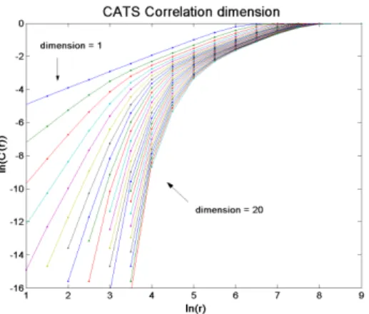
Figure 1 shows the results obtained with the 4900 known values of the CATS time series. With respect to Grassberger-Proccacia’s procedure described above, the data xt are now the p-dimensional regressors defined in (1). The figure shows a plot of ln(C(r)) against ln(r) for increasing dimensions of the data space (i.e. increasing sizes p of the regressors). The expected saturation effect [14] is clear for values of ln(r) between 5 and 8; the correlation dimension seems to be around 1.

Fig. 1. Estimation of the correlation dimension using the Grassberger-Procaccia procedure; log of the correlation integral C(r) versus the log of the hypersphere radius r.

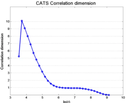
Another representation of the correlation dimension can be given in plotting the estimation of the correlation dimension as in Figure 2. A flat region can be seen around ln(r) = 6 to 7 where the correlation dimension is again ap-proximately one. In conclusion, according to Taken’s theorem, any regressor for the CATS time series should be at most of size 3.

Note that the correlation dimension estimation is only a preliminary rough calculation, in order to get a first insight on the series. Indeed, because of the high correlation between successive values in the series (or in other words its ’smoothness’), it may happen that the correlation dimension estimation just catches this correlation, and not the dynamics of the series. In Figure 1, this could be seen in the form of two saturation effects in the slopes, as detailed above: one when the correlation between successive values is caught, the other one when the true dimensionality of the series is reached. According to the very low value (one) found for the correlation dimension in the CATS series, this risk does not have to be underestimated. Nevertheless, as no other

Fig. 2. Correlation dimension obtained for various values of the hypersphere radius

r (in log scale) for the CATS time series.

reasonable value can be found, we will consider in the following that the value found for the correlation dimension is reliable, and a regressor of size 3 will thus be used.

The problem of a time series with a very low correlation dimension is that each value only depends on the few preceding ones. Any model built accord-ing to the above principles is therefore restricted to a very limited amount of information, and the prediction becomes hard and unstable. This is for exam-ple the case in financial time series prediction: the high sampling frequency of financial indexes makes them extremely smooth at short term. In such con-text, one usually models pre-processed series instead of the original ones; the preprocessing can consist in differences, returns, etc. Because of the similari-ties between the correlation dimension results on such financial series and on the CATS one, the same kind of pre-processing is developed here. In addition to the original series, two pre-processed ones will be used in the experiments: the series obtained by differences and by returns. The difference time series is obtained as:

xd(t) = x(t + 1) − x(t), (4) while the return time series is computed as:

xr(t) =

x(t + 1) − x(t)

x(t) . (5)

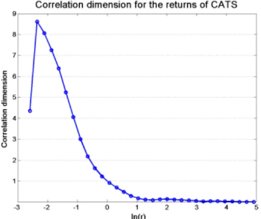
The correlation dimension of these two new time series can also be computed, using the same Grassberger-Procaccia procedure. The results are presented in Figures 3 and 4. Unfortunately, in both cases, the results are not conclu-sive. Indeed there is no visible saturating slope in the ln(C(r)) against ln(r) diagrams, contrarily to the saturation in Figure 2. The results found on the original series will thus be kept in the following as a rough estimation of the correlation dimension of the CATS time series.

Fig. 3. Correlation dimension obtained for various values of the hypersphere radius

r (in log scale) for the difference time series.

Fig. 4. Correlation dimension obtained for various values of the hypersphere radius

r (in log scale) for the return time series.

3 The double quantization forecasting method

3.1 Self-organizing Maps

The Self-Organizing Map (SOM) is an unsupervised classification algorithm introduced in the 80’s by Teuvo Kohonen [3]. Since their first description, Self-Organizing Maps have been applied in many different fields to solve various problems. Their theoretical properties are well established [16], [17].

In a few words, a SOM map has a fixed number of units quantifying the data space. Those units, also called prototypes or centroids, are linked by predefined neighbourhood relationships that can be represented graphically through a 1-or 2-dimensional grid. After learning, the grid of prototypes has two proper-ties. First, it defines a vector quantization of the input space, as any other vector quantization algorithm. Secondly, because the grid relationships are used in the learning algorithm itself, the grid representation has a

topologi-cal property: two close inputs will be projected either on the same prototype or on two close ones in the grid. The Kohonen map can thus be seen as an unfolding procedure or as a nonlinear projection from the data space on a 1-or 2-dimensional grid. The prototypes in a Kohonen map can also be seen as representatives of their associated class (the set of data nearer from a specific prototype than from any other one), turning the algorithm into a classification (or at least a clustering) tool. One of the main features of Kohonen maps is their ability to easily project data in a 2-dimensional representation, allowing intuitive interpretations.

3.2 The Double Vector Quantization method (DVQ)

Though the SOM is usually considered as a classification, feature extraction or recognition tool, there exist a few works where the SOM algorithm is used in time series prediction problems, as [5],[6], [12], [4], [8], [7]. In most of these situations however, the goal is to reach a reliable one-step-ahead prediction. In this work we are specifically looking for longer-term ones, and more precisely to 20 steps ahead prediction in the context of the CATS Competition.

A complete description of the DVQ method is given in [1], together with a full proof of the method stability for long-term predictions. A brief description of the method is given here in the simple case of a scalar time series prediction. Full details for the vector case can be found in [1]. The goal of the method is to extract long-term information or trends of a time series. The method is based on the SOM algorithm used to characterize (or learn) the past of the series. Afterwards a forecasting step allows predicting future values.

3.2.1 Characterization

According to the formulation of a nonlinear auto-regressive model (1), the method uses regressors of past values to predict the future evolution of a time series. Having at disposal a scalar time series of n values, the correlation dimension Dc is evaluated, leading to the choice of p-dimensional regressors. The n known values of the time series are then transformed into p-dimensional regressors:

xt= {x(t − p + 1), ..., x(t − 1), x(t)}, (6) where p ≤ t ≤ n, and x(t) is the original time series at our disposal. As one may expect n−p+1 such regressors are obtained from the original time series. The original regressors xtare then manipulated such that other regressors are created, according to:

The yt vectors are called the deformation regressors, or the deformations in short. By definition each deformation yt is associated to a single regressor xt. Of course, n − p deformations are obtained from a time series of n values. At this stage of the method there exist two sets of regressors. The first one contains the xt regressors and is representative of the original space (of re-gressors). The space containing the yt deformations is representative of the deformation space. Those two sets of vectors, of the same dimension p, will be the data manipulated by the SOM maps.

Applying the SOM algorithm to each one of these two sets results in two sets of prototypes, denoted respectively ¯xi, with 1 ≤ i ≤ n1, and ¯yj, with 1 ≤ j ≤ n2. The classes associated to those prototypes are denoted respectively ci and c′j. Characterizing the two time series through the quantization of the regressors and deformations is a static-only process. The dynamics of the past evolution of the series has to be modeled too. In fact, this is possible because the dy-namics is implicitly recorded in the deformations. The issue is thus to build a representation of the existing relations between the original regressors and the deformations. For this purpose, a matrix f (ij) is defined such that its ij element, denoted fij, is obtained as:

fij =

#{xt ∈ ci and yt∈ c′j} #{xt ∈ ci}

, (8)

with 1 ≤ i ≤ n1, 1 ≤ j ≤ n2. Intuitively the probability of having a certain deformation j associated to a given regressor i is approximated by the empir-ical frequencies (8) measured on the data at disposal. Each row of the f (ij) matrix (1 ≤ j ≤ n2) in (8) is in fact the conditional probability that ytbelongs to c′

j given the fact that xt belongs to ci. Of course, elements fij (1 ≤ j ≤ n2) sum to one for each i.

3.2.2 Forecasting

Now that the past evolution of the time series has been modeled, predictions can be performed. Let us define the last known value x(t) at time t, with corresponding regressor xt. The prototype ¯xkclosest to xtin the original space is searched. According to the conditional probability distribution defined by row k, a deformation prototype ¯yl is then chosen randomly among the ¯yj, according to the fkj probability law. The prediction for instant t + 1 is finally obtained according to relation (7):

ˆ

xt+1 = xt+ ¯yl, (9)

where ˆxt+1 is the estimate of xt+1 given by the model. In fact ˆxt+1 is a p-dimensional vector, and only one of its components corresponds to a prediction

ˆ

x(t + 1) at time t + 1; this value is thus extracted from the ˆxt+1 vector and taken as the prediction.

Once a one-step-ahead prediction (horizon h = 1) is computed, the whole procedure can be repeated to obtain predictions for higher values of h. In practice, prediction ˆx(t + 1) is used to compute ˆxt+2 through its corresponding regressor ˆxt+1. ˆx(t + 2) is then extracted from ˆxt+2, and so on up to horizon h. This recursive procedure is the standard way to obtain long-term forecasts from a one-step-ahead method. The whole procedure up to horizon h is called a simulation.

3.2.3 Comments

The goal of the DVQ method is to provide insights over the possible long-term evolution of a series, and not necessarily a single accurate prediction. The long-term (horizon h) simulations are then repeated using a Monte-Carlo procedure. The simulations distribution can be observed, and statistical information such as variance, confidence intervals, etc. can be determined too. The obtained long-term predictions have been proven to be stable [1].

Another important comment is that the method can easily be generalized to the prediction of vectors. With respect to the procedure described in the previ-ous subsection, the only difference is that deformations (7) must be computed by differences of d-spaced values:

yt= xt+d− xt, (10)

a direct generalization of the d = 1 case in (7). Then, d scalar values have to be extracted from the ˆxt+d vector, and so on. For example, two values could be extracted (corresponding to ˆx(t + 1) and ˆx(t + 2)). In this case, repeating the procedure means to inject ˆx(t + 1) and ˆx(t + 2) to predict ˆx(t + 3) and ˆ

x(t + 4). More details about the vector case can be found in [1].

A third comment concerns the numbers n1 and n2 of prototypes respectively in the regressor and deformation spaces. The major concern is that different values of n1 (n2) lead to different segmentations of the regressor and the de-formation spaces which in turn lead to different models of the time series. The values of n1 and n2 should therefore be optimized, for example by resampling procedures (cross-validation, bootstrap) on a predefined error criterion, as the one-step-ahead error.

Finally, since the only property of the SOM used here is the vector quan-tization, any other vector quantization method could have been chosen to implement the above procedure. The SOM maps have been chosen since they seem more efficient and faster compared to other VQ methods despite a limited

complexity [18]. Furthermore, they provide an intuitive and helpful graphical representation. Note that in practice any kind of SOM map could be used, but that one-dimensional maps, or strings, are preferred here.

4 Methodological aspects of the double quantization for the CATS data set

As mentioned in section 3.2 the goal of the DVQ method is to provide insights over the possible long-term evolution of a series, and not necessarily a single accurate prediction. In this section the methodology for the experiments will be described having in mind that the method has now to predict accurate values due to the competition context.

4.1 Scalar and vector predictions

From section 2 we know that regressor xt for nonlinear models should contain at most 3 past values:

xt = {x(t − 2), x(t − 1), x(t)}. (11) As this expression has the same form as relation (6), it allows a direct appli-cation of the DVQ method to predict x(t + 1). This direct appliappli-cation of the method is an illustration of the scalar prediction with the DVQ method. The use of the correlation dimension to set the size of the regressor should however be taken with care when predicting vectors instead of scalars, as it will be the case for the CATS series. As an example, if one wants to predict a vector of d = 2 values, namely {ˆx(t + 1), ˆx(t + 2)}, the following two regressors should be respectively used:

{x(t − 2), x(t − 1), x(t)} to predict ˆx(t + 1),

{x(t − 1), x(t), x(t + 1)} to predict ˆx(t + 2). (12) In order to use the DVQ method, it is suggested to merge the two regressors and use:

{x(t − 2), x(t − 1), x(t), x(t + 1)} (13) to predict {ˆx(t + 1), ˆx(t + 2)} together. Of course this is impossible since value x(t + 1) is unknown at time t. Therefore, the regressors that will be used in the following have the same size as in Eq. 13 but they are shifted such that their last component now corresponds to x(t):

In this example, deformations yt are then computed according to: yt = xt+d - xt

= {x(t − 1), x(t), x(t + 1), x(t + 2)} - {x(t − 3), x(t − 2), x(t − 1), x(t)}.

(15)

The same procedure can be extended for values of d greater than 2.

To summarize, the DVQ method is directly applicable in the scalar case. Some care must be taken in the vector case: if vectors of d values have to be predicted then the corresponding regressors have to be merged into a single vector which may only contain known values. Only then, the DVQ method in vector case can be applied.

4.2 20 step ahead prediction strategies

As the CATS competition requires predicting block of 20 successive unknown values, several strategies can be used to reach this prediction horizon. The first one, called the recursive strategy, is probably the most common way to obtain a long term prediction. Predictions are obtained recursively until the final time horizon h; i. e. the one-step-ahead predictions are included one by one in the regressor to obtain the next one-step-ahead prediction. Formally, the last prediction ˆx(t + k) is used to predict the next one ˆx(t + k + 1) as part of the regressor for t + k + 1 (1 ≤ k ≤ d − 1).

The second approach, called the block strategy, consists in predicting all the h future values in one single vector. This is made possible by the use of a vector prediction method, as the DVQ one.

A mixed approach is a recursive-block strategy, where blocks of intermediate size d are predicted through a limited number of h/d recursive steps (where h is supposed to be a multiple of d for simplicity).

4.3 Number of prototypes

As mentioned in section 3.2, the numbers n1 and n2 of prototypes in respec-tively the regressor and the deformation spaces have to be fixed. A cross-validation procedure is therefore used. This cross-cross-validation procedure mimics the competition problem.

data. As the true values for those 300 new missing values are known they can serve as validation set for models learned on the remaining values. Note that the random selection was slightly constrained: the new gaps could not overlap between them and with the existing ones. The whole validation procedure has been repeated 20 times, to average the dependencies to the choice of the 300 new gaps.

To compare the different models that will be learned on the 20 various learning sets a mean square error MSE validation criterion is used. This criterion is comparable to the one proposed in the CATS competition and is defined as:

MSE =

X

yt∈V S

(yt− ˆyt)2

300 , (16)

where V S represents one of the 20 validation sets of 300 new missing values. The best model will be the one which has the lowest average MSE over the 20 validation sets.

4.4 Final predictions

Once the optimal n1 and n2 numbers are found, a new learning stage is done now using all available data (i.e. the 4900 data of the original CATS time series).

To avoid problems due to the random initialization of the prototypes, several learning procedures are performed, and the best one is selected according to the validation sets, even if using the latter may lead to a small amount of overfitting (as the validation sets are now part of the new learning set). Simulations at final horizon are then repeated 100 times, and the mean is computed.

To refine this direct application of the DVQ method to the CATS predic-tion problem, some specific heuristics have been developed. The first one is to reverse the time series. Indeed, for the four blocks inside the series, the prediction can be performed from right to left (decreasing values of time) as well as it is performed from left to right (chronological order). For those four blocks of length 20, the CATS Competition is a missing value problem rather than a forecasting one. The DVQ method will therefore be applied in both directions.

The second heuristic considers a prediction horizon up to h = 21 (instead of h = 20). Indeed, as the 21st value is known for the four first gaps, predicting to horizon h = 21 allows a comparison between the true value and the 21st pre-dicted one. As some error in long-term trends of the prediction is unavoidable,

the comparison between these true and predicted values leads to an error that can be compensated at first order through a linear correction of the simulated predictions. This correction is performed such that the 21st predicted value is made equal to the true one.

The final predictions that were sent to the Competition were obtained by the DVQ method combined with the two heuristics explained above. More precisely, for the four first blocks of 20 missing values, a prediction to horizon h = 21 was performed in both directions, resulting from 100 DVQ simulations. As the true value for the 21st data is known in both directions for these four cases, a linear correction has been applied. The final predictions were then obtained as the average of the two linearly corrected predictions.

Of course, as the true 21st value is unknown for the fifth block of missing data, the above strategy can not be applied. The final predictions for this case were obtained as the mean of 100 DVQ simulations.

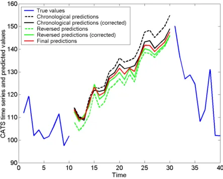
Figure 5 shows the various steps leading to the final predictions for the first block of missing values. The outmost curves are the mean of the 100 DVQ simulations (top of the figure is the chronological order, bottom is the re-versed order). The two inner curves are the linearly corrected values using the comparison between the 21st true and predicted values. The fifth curve in the middle represents the final predictions, i.e. the mean of the two (linearly corrected) inner curves.

Fig. 5. Corrections applied to obtain the final predictions using the two heuristics (first block of missing values; data 981-1000). See text for details.

5 Experimental results

According to the ’financial-like’ behaviour of the CATS time series, as dis-cussed in section 2, three time series are considered in all our experiments: the initial CATS, the difference and the return time series. Furthermore, this ’financial-like’ behaviour already suggests that a recursive strategy may be-have poorly for a time horizon of 20 values. Consequently, in addition to the recursive strategy, where one-step-ahead predictions are repeated 20 times, a recursive-block strategy is used, with blocks of size 2, 5 and 10, and finally a block strategy is used with a bloc size equal to the time horizon h = 20. In the recursive-block strategy, the time horizon of 20 values corresponds to predict 10 blocks of size d = 2, 4 blocks of size 5, etc.

For each one of the three time series, for each one of the block sizes, a cross-validation using the 20 cross-validation sets has been performed as described in section 4.3. For comparison purposes the new missing values in the 20 valida-tion sets are identical in all experiments. Models with n1 and n2 both ranging from 5 to 100 by incremental steps of 5 are learned in each experiment. The MSE criterion (16) has been used to estimate the models generalization abil-ity on the validation sets.

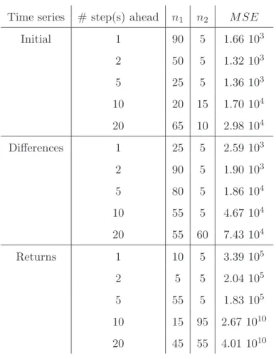
Table 1 gives a summary of the experiments. For each time series, for each block size, n1 and n2 corresponding to the best model in average are given, together with the average MSE. For the difference and return time series the MSE is of course computed by first applying the inverse transformations on the predictions, in order to obtain MSE values that can be compared between the series.

From this table it seems clear that a model learned on the initial time series is adequate; none of the two preprocessing methods suggested in (4) and (5) reveals interesting. Indeed the MSE values obtained on the validation sets are in both cases larger than those obtained with the initial time series.

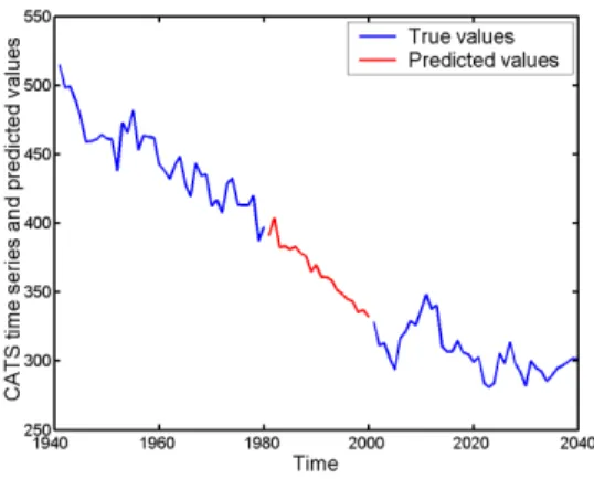
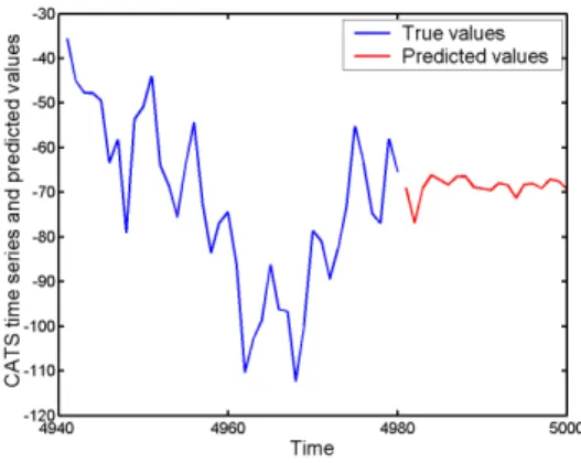
Furthermore it is obvious that there exists a compromise between 20 repeti-tions of a one-step-ahead prediction (recursive strategy) and a single prediction of a vector containing the 20 next values (block strategy). This compromise seems to be somewhere between 10 predictions of blocks of 2 values and 4 predictions of blocks of 5 values. Nowadays the MSE criterion is the lowest for blocks of size d = 2. The corresponding model, with 50 prototypes in the regressor space and 5 in the deformation space, is selected to give the final prediction of the 100 missing values of the CATS Competition according to the heuristic described in section 4.4. Figures 6 to 10 show how the DVQ method predicts the missing values for the five 20-values blocks of the CATS competition.

Time series # step(s) ahead n1 n2 M SE Initial 1 90 5 1.66 103 2 50 5 1.32 103 5 25 5 1.36 103 10 20 15 1.70 104 20 65 10 2.98 104 Differences 1 25 5 2.59 103 2 90 5 1.90 103 5 80 5 1.86 104 10 55 5 4.67 104 20 55 60 7.43 104 Returns 1 10 5 3.39 105 2 5 5 2.04 105 5 55 5 1.83 105 10 15 95 2.67 1010 20 45 55 4.01 1010 Table 1

Experiment summary: n1 and n2 for the best model in average over the 20

cross-validations and corresponding M SE.

Fig. 6. True values and final predictions, first gap.

After the CATS Competition was closed, the results of the 17 classified com-petitors out of the 24 submissions were made available [2]. It can be seen in [2] that the DVQ method was ranked to the fourth position on the problem of predicting the first four gaps of 20 missing data. The value of the E2 criterion in [2] (average sum of squares of errors on first 80 missing data) is 351. Besides the efficiency of the forecasting method, this is probably, and not surprisingly,

Fig. 7. True values and final predictions, second gap.

Fig. 8. True values and final predictions, third gap.

Fig. 9. True values and final predictions, fourth gap.

a consequence of the fact that taking into account the first known value af-ter each gap indeed improves the prediction accuracy. This information is not available for the fifth block of 20 missing data. The E1 criterion in [2] (average sum of squares of errors on the 100 missing data) takes into account this very different problem. On this criterion, the DVQ method performs slightly worst with a result of 653, and is ranked in seventh position.

Fig. 10. True values and final predictions, fifth gap.

6 Conclusion

In this paper the results obtained with the double vector quantization method, based on the SOM maps, applied to the CATS data set are presented.

An analysis of the data shows some interesting aspects of the time series. Its correlation dimension seems to be as low as one. To take into account this particular aspect potentially limiting for nonlinear models other time series have been defined, i.e. the differences and the returns of the initial CATS series.

These three time series have been modeled using various sizes of prediction blocks corresponding to longer time horizons, in order to make the most of the vector prediction ability of the double vector quantization method. The number of units in the SOM maps has been discussed and selected using a cross-validation procedure on new gaps created randomly on the CATS data set. This procedure, together with the selected validation criterion, has been implemented to select the best model in average in conditions as close as possible to the Competition ones.

Heuristics specifically designed in the CATS Competition context are also described.

Finally, the predictions obtained using the best selected model and the heuris-tics are illustrated graphically.

Acknowledgements

G. Simon is funded by the Belgian F.R.I.A., M. Verleysen is Senior Research Associate of the Belgian F.N.R.S. The scientific responsibility rests with the authors.

References

[1] G. Simon, A. Lendasse, M. Cottrell, J.-C. Fort, M. Verleysen, Double quantization of the regressor space for long-term time series prediction: Method and proof of stability, Neural Networks, Elsevier, Vol. 17, Nos. 8-9 (October-November 2004), pp. 1169-1181.

[2] A. Lendasse, E. Oja, O. Simula, M. Verleysen, Time Series Prediction Competition: The CATS Benchmark, in Proc. of IJCNN’2004, July 2004, Budapest (Hungary), IEEE, pp. 1615-1620.

[3] T. Kohonen, Self-organising Maps, Springer Series in Information Sciences, Vol. 30, Springer, Berlin, 1995.

[4] M. Cottrell, E. de Bodt, Ph. Gr´egoire, Simulating Interest Rate Structure Evolution on a Long Term Horizon: A Kohonen Map Application, in Proc. of Neural Networks in The Capital Markets, Californian Institute of Technology, World Scientific Ed., Pasadena, 1996.

[5] J. Walter, H. Ritter, K. Schulten, Non-linear prediction with self-organising maps, in Proc. of IJCNN, San Diego, CA, 589-594, July 1990.

[6] J. Vesanto, Using the SOM and Local Models in Time-Series Prediction, in Proc. of Workshop on Self-Organizing Maps (WSOM’97), Espoo (Finland), pp. 209-214, 1997.

[7] S. Dablemont, G. Simon, A. Lendasse, A. Ruttiens, F. Blayo, M. Verleysen, Time series forecasting with SOM and local non-linear models - Application to the DAX30 index prediction, in Proc. of Workshop on Self-Organizing Maps WSOM’03, septembre 2003, Kitakyushu (Japan), pp. 340-345.

[8] M. Cottrell, B. Girard, P. Rousset, Forecasting of curves using a Kohonen classification, Journal of Forecasting, Vol. 17, pp. 429-439, 1998.

[9] T. Voegtlin, Recursive Self-Organizing Maps, Neural Networks, 15(8-9), pp. 979-991, 2002.

[10] G. J. Chappell, G. J. Taylor, The temporal Kohonen map, Neural Networks, 6, pp. 441-445, 1993.

[11] J. Kangas, On the Analysis of Pattern Sequences by SelfOrganizing Maps, Ph. D. thesis, Helsinki University of Technology, 1994.

[12] T. Koskela, M. Varsta, J. Heikkonen, K. Kaski, Recurrent SOM with Local Linear Models in Time Series Prediction, in Proc. of European Symp. on Artificial Neural Networks, April 1998, Bruges (Belgium), D-Facto pub. (Brussels), pp. 167-172.

[13] P. Grassberger, I. Procaccia, Measuring the strangeness of strange attractors, Physica, Vol. D9, pp. 189-208, 1983.

[14] F. Camastra, A. M. Colla, Neural Short-Term Prediction Based on Dynamics Reconstruction, Neural Processing Letters, n. 9, Vol. 1, pp. 45-52, 1999. [15] F. Takens, Detecting strange attractors in turbulence, in Dynamical Systems

and turbulence - Warwick, 1980, Lecture Notes in Mathematics 898, Springer-Verlag, 1981.

[16] M. Cottrell, J.-C. Fort, G. Pag`es, Theoretical aspects of the SOM algorithm, Neurocomputing, 21, pp. 119-138, 1998.

[17] M. Cottrell, E. de Bodt, M. Verleysen, Kohonen maps versus vector quantization for data analysis, in Proc. of European Symp. on Artificial Neural Networks, April 1997, Bruges (Belgium), D-Facto pub. (Brussels), pp. 187-193.

[18] E. de Bodt, M. Cottrell, P. Letremy, M. Verleysen, On the use of Self-Organizing Maps to accelerate vector quantization, Accepted for publication in Neurocomputing, Elsevier.

Geoffroy Simon was born in 1978 in Dinant, Belgium. He

re-ceived the M.Sc. degree in Computer Sciences in 2002 from the Facult´es Universitaires Notre Dame de la Paix (Namur, Belgium). He is now working as Ph. D. student at the Microelectronic Labo-ratory of the Electrical Engineering Departement of the Universit´e catholique de Louvain (UCL). His research topics cover nonlinear time series analysis, artificial neural networks, nonlinear statistics and self-organization applied to time-series forecasting problems. He is currently member of the UCL Machine Learning Group. His work is funded by a grant from the Belgian F.R.I.A. (Fonds pour la formation la Recherche dans l’Industrie et dans l’Agriculture).

John Aldo Lee was born in 1976 in Brussels, Belgium. He

re-ceived the M.Sc. degree in Applied Sciences (Computer Engineer-ing) in 1999 and the Ph.D. degree in Applied Sciences (Machine Learning) in 2003, both from the Universit´e catholique de Louvain (UCL, Belgium). His main interests are nonlinear dimensionality reduction, intrinsic dimensionality estimation, independent com-ponent analysis, clustering and vector quantization. He is a former member of the UCL Machine Learning Group and is now a Sci-entific Research Worker of the Belgian F.N.R.S. (Fonds National de la Recherche Scientifique). His current work aims at developing specific image enhancement tech-niques for Positron Emission Tomography in the Molecular Imaging and Experi-mental Radiotherapy department of the Saint-Luc University Hospital (Belgium).

Marie Cottrell was born in 1943 in B´ethune, France. She was a student at the Ecole Normale Sup´erieure de S`evres, and received the Agr´egation de Math´ematiques degree in 1964 (with 8th place), and the Th`ese d’Etat (Mod´elisations de r´eseaux de neurones par des chaˆines de Markov et autres applications) in 1988. From 1964 to 1967, she was a High School Teacher. From 1967 to 1988, she was successively an Assistant and an Assistant Professor at the Uni-versity of Paris and at the UniUni-versity of Paris-Sud (Orsay), except from 1970 to 1973, on which she was a Professor at the University of Havana, Cuba. From 1989, she is a full Professor at the University Paris 1 - Panth´eon-Sorbonne. Her research interests include stochastic algorithms, large deviation theory, biomathe-matics, data analysis and statistics. Since 1986, her main works deal with artificial and biological neural networks, Kohonen maps and their applications in data anal-ysis. She is the author of about 80 publications in this field. She is in charge of the SAMOS research group at the University Paris 1. She is regularly solicited as referee or international conference program committee member. In 2005, she organized the Fifth WSOM Conference in Paris.

Michel Verleysen was born in 1965 in Belgium. He received

the M.S. and Ph.D. degrees in electrical engineering from the Uni-versit´e catholique de Louvain (Belgium) in 1987 and 1992, respec-tively. He was an Invited Professor at the Swiss E.P.F.L. (Ecole Polytechnique F´ed´erale de Lausanne, Switzerland) in 1992, at the Universit´e d’Evry Val d’Essonne (France) in 2001, and at the Uni-versit´e Paris 1 - Panth´eon-Sorbonne in 2002, 2003 and 2004. He is now a Research Director of the Belgian F.N.R.S. (Fonds National de la Recherche Scientique) and Lecturer at the Universit´e catholique de Louvain. He is editor-in-chief of the Neural Processing Letters journal, chairman of the annual ESANN conference (European Symposium on Artificial Neural Networks), associate editor of the IEEE Trans. on Neural Networks journal, and member of the edito-rial board and program committee of several journals and conferences on neural networks and learning. He is author or co-author of about 200 scientific papers in international journals and books or communications to conferences with reviewing committee. He is the co-author of the scientific popularization book on artificial neural networks in the series ”Que Sais-Je?”, in French. His research interests in-clude machine learning, artificial neural networks, self-organization, time-series fore-casting, nonlinear statistics, adaptive signal processing, and high-dimensional data analysis.