Thesis No 2495
DOCTORAL THESIS
Submitted byEl Mehdi ISMAILI ALAOUI
Discipline : Engineering Science
Speciality : Computer Science, Telecommunications and Multimedia
N
EW
R
OBUST
T
ECHNIQUES FOR
M
OTION
E
STIMATION AND
S
EGMENTATION OF
M
OVING
O
BJECTS IN
V
IDEO
S
EQUENCE
Defended on May 29th2010
Thesis committee:
President:
El Houssine BOUYAKHF Professor (PES), Faculty of Sciences (Rabat)
Examiners:
Elhassane IBN-ELHAJ Professor (PH), INPT (Rabat)
Fakhita REGRAGUI Professor (PES), Faculty of Sciences (Rabat)
Ahmed TAMTAOUI Professor (PES), INPT (Rabat)
Driss MAMMASS Professor (PES), Faculty of Sciences (Agadir)
Hassan QJIDAA Professor (PES), Faculty of Sciences (Fes)
Faculté des Sciences, 4 Avenue Ibn Battouta B.P. 1014 RP, Rabat, Maroc Tel : +212 (0) 37 77 18 34/35/38, Fax : +212 (0) 37 77 42 61, http://www.fsr.ac.ma
Ce mémoire de thèse a été réalisé au sein du Laboratoire Informatique, Mathématiques appliquées, In-telligence Artificielle et Reconnaissance de Formes (LIMIARF) de la Faculté des Sciences Agdal, Rabat.
Les travaux de recherche présentés dans cette thèse ont été réalisés en collaboration avec le laboratoire de traitement d’images de l’Institut National des Postes et Télécommunication (INPT-Rabat).
En premier lieu, je tiens à exprimer ma gratitude à Monsieur El Houssaine BOUYAKHF, professeur à la Faculté des Sciences de Rabat et directeur de l’unité Architecture et Conception de Systèmes informatiques (ACSYS), pour m’avoir accueilli au sein de son laboratoire LIMIARF, pour son aide et pour l’honneur qu’il me fait en présidant mon jury de thèse.
Je remercie Monsieur Elhassane IBNELHAJ, professeur à l’INPT de Rabat, pour m’avoir donné l’opportu-nité d’entreprendre ce travail au sein du laboratoire de traitement d’images de l’INPT. Ces années passées à cet institut m’ont apporté une expérience extrêmement enrichissante, aussi bien sur les plans culturel et humain. Je le remercie également pour avoir dirigé et encadré ce travail avec une grande rigueur scientifique. La qualité de ses conseils, le soutien et la confiance qu’il m’a accordés, m’ont permis de faire évoluer mes idées et de me donner une autre vision de la recherche.
J’aimerais également remercier Madame Fakhita REGRAGUI, professeur à la Faculté des Sciences de Ra-bat, et Monsieur Ahmed TAMTAOUI, professeur à l’INPT de RaRa-bat, d’avoir accepté la lourde tâche de rapporteur et d’avoir consacré un temps précieux à l’examen de ce manuscrit. La qualité et la précision de leurs remarques m’ont permis de l’améliorer .
Je tiens ensuite à remercier Monsieur Driss MAMMASS, professeur à la Faculté des Sciences d’Agadir et Monsieur Hassan QJIDAA, professeur à la Faculté des Sciences de Fes, pour avoir accepté d’examiner cette
Ces remerciements ne seraient pas complets sans y associer ma famille. Je remercie tout d’abord mes parents pour leur énorme soutien moral et matériel, leur présence et leurs encouragements pendant toute la période de mes études. Je remercie également mes deux frères et ma soeur pour m’avoir toujours soutenu.
Finalement, je remercie tous ceux que je n’ai pas cités (amis, famille, chercheurs,...) et qui ont contribué, d’une façon ou d’une autre, à la réussite de cette "aventure".
Table of Contents vii
List of Figures xi
List of Tables xiii
Chapter 1 : Introduction 1
1. 1 Background of research . . . 1
1. 2 Motion detection . . . 2
1. 2. 1 Motion estimation . . . 2
1. 2. 2 Segmentation of moving objects . . . 2
1. 3 Motivation of the research . . . 3
1. 4 Contribution of the research . . . 5
1. 5 Thesis organization . . . 6
Chapter 2 : Motion Estimation Techniques: State of the art 9 2. 1 Introduction . . . 10
2. 2 Motion representation . . . 11
2. 3 Characterization of the motion . . . 12
2. 3. 1 Pan motion . . . 12
2. 3. 2 Tilt motion . . . 13
2. 3. 3 Rotary motion . . . 13
2. 3. 4 Zoom motion . . . 13
2. 4 Motion models . . . 14
2. 4. 1 Rigid body motion . . . 15
2. 5 Region of support for motion representation . . . 16
2. 6 Interdependence of motion and image data . . . 18
2. 7 Estimation criteria . . . 19
2. 7. 1 DFD-based criteria . . . 19
2. 7. 2 Frequency domain criteria . . . 20
2. 7. 3 Bayesian criteria . . . 21
2. 8 A review of motion estimation techniques . . . 22
2. 8. 1 Gradient techniques . . . 22
2. 8. 2 Pel-recursive techniques . . . 24
2. 8. 3 Block matching techniques . . . 25
2. 8. 4 Frequency domain techniques . . . 26
2. 9 Conclusion . . . 29
Chapter 3 : Higher-Order Spectra: Definitions, Properties, and Applications 31 3. 1 Introduction . . . 32
3. 1. 1 Moments and cumulants . . . 32
3. 1. 2 Relationship between moments and cumulants . . . 33
3. 1. 3 Moments and cumulants of stationary processes . . . 34
3. 1. 4 Moments versus cumulants . . . 35
3. 1. 5 The relationship between cumulant functions and HOS . . . 36
3. 1. 6 Properties of moments and cumulants . . . 36
3. 1. 7 HOS of the frequency domain . . . 38
3. 1. 7. 1 Power and energy spectra . . . 38
3. 1. 7. 2 The bispectrum . . . 39
3. 2 Applications of HOS in image processing . . . 40
3. 2. 1 Image reconstruction . . . 40
3. 2. 2 Texture classification . . . 40
3. 2. 3 Invariant pattern recognition . . . 41
3. 2. 4 Image restoration . . . 42
3. 3 Conclusion . . . 43
Chapter 4 : New Motion Estimation Techniques using Higher-Order Spectra 45 4. 1 Introduction . . . 46
4. 1. 1 Problem formulation . . . 46
4. 2 The proposed bispectrum-based image motion estimation . . . 47
4. 2. 1. 1 Definitions and properties . . . 47
4. 2. 1. 2 Symmetry properties of the bispectrum . . . 50
4. 2. 2 Translation model in the bispectrum domain . . . 50
4. 2. 3 Extension to sub-pixel motion estimation . . . 52
4. 2. 3. 1 Parabolic interpolation . . . 52
4. 2. 4 Parametric bispectrum method . . . 53
4. 3 Experimental results and discussion . . . 56
4. 4 Conclusion . . . 63
Chapter 5 : Hierarchical Motion Estimation Using an Affine Model in the Bispectrum Domain 65 5. 1 Introduction . . . 66
5. 2 A hierarchical affine approach . . . 66
5. 2. 1 An affine motion model in the bispectrum domain . . . 67
5. 2. 2 Hierarchical motion estimation . . . 70
5. 2. 2. 1 Pyramid construction . . . 71
5. 2. 2. 2 Global motion estimation . . . 71
5. 2. 2. 3 Local motion estimation . . . 72
5. 3 Computational cost . . . 74
5. 4 Experimental results and discussion . . . 74
5. 5 Conclusion . . . 80
Chapter 6 : Segmentation of Moving Objects in a Sequence of Video Images 81 6. 1 Introduction . . . 82
6. 2 Problems related to segmentation of moving objects . . . 82
6. 3 Segmentation of moving objects: an overview . . . 83
6. 3. 1 Motion-based segmentation . . . 83
6. 3. 2 Spatio-temporal video segmentation . . . 85
6. 3. 2. 1 Segmentation based on motion information only . . . 85
6. 3. 2. 2 Segmentation based on motion and spatial information . . . 86
6. 3. 2. 3 Segmentation based on change detection . . . 87
6. 3. 2. 4 Segmentation based on edge detection . . . 89
6. 3. 3 Statistical approaches . . . 90
6. 3. 4 Dominant motion analysis . . . 91
Chapter 7 : Robust Higher-Order Spectra for Motion Segmentation of Video Sequences 95
7. 1 Introduction . . . 96
7. 2 The proposed motion segmentation approach . . . 97
7. 2. 1 Multiple motion estimation . . . 97
7. 2. 2 Temporal coherence . . . 98
7. 2. 3 HOS-based decision measure . . . 98
7. 2. 4 HOS-based k-means clustering . . . 99
7. 2. 5 Implementation . . . 99
7. 2. 5. 1 Dense motion estimation . . . 100
7. 2. 5. 2 Model generator . . . 100
7. 2. 5. 3 Model estimator . . . 101
7. 2. 5. 4 Model merger based on motion . . . 101
7. 2. 5. 5 Model classifier . . . 102
7. 2. 5. 6 Model splitter . . . 103
7. 2. 5. 7 Model filter . . . 103
7. 2. 5. 8 Iterative algorithm . . . 103
7. 2. 5. 9 Extraction foreground/backgroun . . . 103
7. 3 Experimental results and discussion . . . 104
7. 4 Conclusion . . . 109
Chapter 8 : Conclusion and Suggested Future Research 111 8. 1 Summary and conclusion . . . 111
8. 2 Direction of future research . . . 113
8. 3 Overview publications . . . 114
8. 3. 1 International journals and chapter books . . . 114
8. 3. 2 International conferences . . . 114
8. 3. 3 National conferences . . . 115
Glossary 119
Bibliography 121
2.1 The 2-D projection of the movement of a point in the 3-D real world is referred as the motion. 11
2.2 A typical 2-D motion field between two frames. . . 12
2.3 Typical types of camera motion. . . 14
4.1 Physical representation of cumulants [BRS97]. . . 48
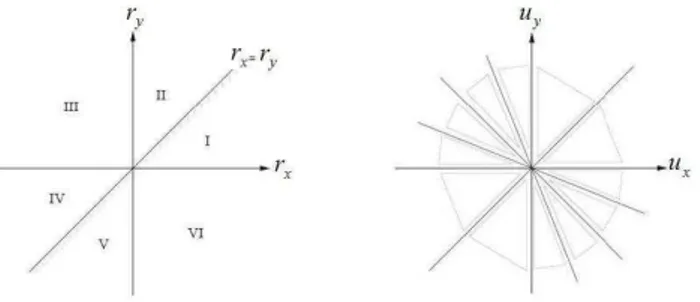
4.2 Symmetry regions of third-order cumulants and bispectrum. . . 50
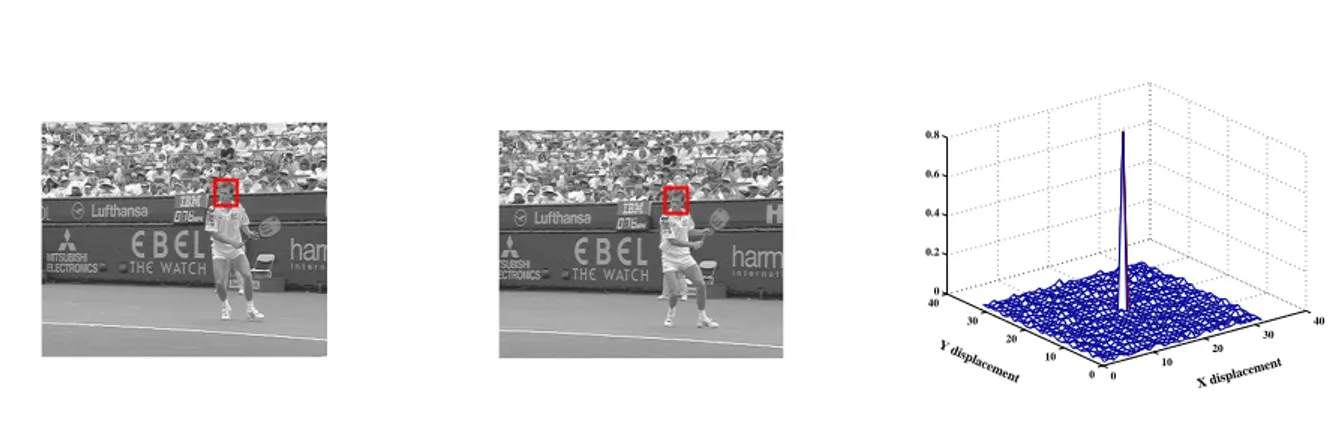
4.3 The correlation surface between the block bt(x, y) and its reference bt−1(x, y) related to frames 2 and 3 of the Stefan sequence respectively. . . . 52
4.4 An illustration of the parabolic fitting. . . 53
4.5 Motion field for the Hall Monitor sequence in the presence of ACGN. . . . 57
4.6 Motion field for the Beanbags sequence in the presence of ACGN. . . . 57
4.7 MSE vs frame number performance comparison with phase correlation method. . . 58
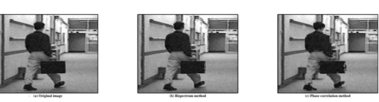
4.8 Prediction for frame 44 of the Hall Monitor sequence in the presence of ACGN. . . . 58
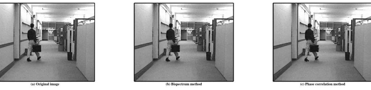
4.9 Enlarged portions of the motion compensated pictures of the Hall Monitor sequence. . . . . 59
4.10 Correlation surfaces between two blocks. . . 59
4.11 PSNR versus frame number for motion compensated prediction. . . 60
4.12 Original and reconstructed frames by each algorithm. . . 61
4.13 Motion field for the Flower Garden sequence in the presence of ACGN. . . . 61
4.14 PSNR versus frame number for motion compensated prediction of the Miss America sequence. 62 4.15 Motion field for the Grove sequence in the presence of ACGN. . . . 62
4.16 Motion field for the Stefan sequence in the presence of ACGN. . . . 62
4.17 Prediction for frame 70 of the Table Tennis sequence in the presence of ACGN. . . . 63
5.2 Illustration of the hierarchical approach to global motion estimation. Initially, motion vec-tors are estimated on a downscaled version of the image. The resulting vecvec-tors initialize a
refinement at the next higher resolution. . . 72
5.3 Local motion estimation steps. . . 73
5.4 The improvement of motion estimation accuracy (dB). . . 75
5.5 PSNR obtained for the noisy sequences. . . 76
5.6 Motion field for the Silent sequence in the presence of ACGN. . . . 76
5.7 Motion field for the Table Tennis sequence in the presence of ACGN. . . . 77
5.8 Portion of zooming motion for two frames from the Table Tennis sequence. . . . 77
5.9 PSNR (average) vs source (SNR). . . 78
5.10 PSNR obtained for the noisy sequences. . . 79
6.1 (a) Simplified motion-based segmentation and (b) simplified spatio-temporal segmentation [ZL01]. . . 84
6.2 Block diagram of the change detector. (C, Ci: change detection masks) [ZL01] . . . 89
7.1 Block diagram of the motion segmentation algorithm. . . 100
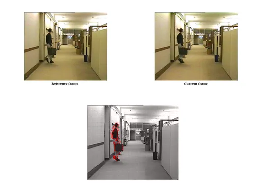
7.2 Video objects segmentation for Hall Monitor sequence (CIF, frame: 93, 131 and 203). . . . . 105
7.3 Video objects segmentation for Table Tennis sequence (SIF, frame: 55, 73 and 102). . . . 106
7.4 Video objects segmentation for Mother & Daughter sequence (CIF, frame: 70, 86 and 181). . 107
7.5 Video objects segmentation for Miss America sequence (QCIF, frame: 55, 91 and 114). . . . 108
4. 1 Time-averaged MSE performance comparison with the SPPCA. . . 60
5. 1 The improvement of motion estimation accuracy (dB). . . 75
5. 2 Average PSNR of motion compensated images for the two motion estimation techniques (dB). 79
I
NTRODUCTION
—————————————–Science must begin with myths, and with the criticism of myths.
————————- ———————————————————-Karl R. Popper (1902-1994)
1. 1 Background of research
V
ideo processing is today one of the most important research field among multimedia types because of its large number of applications. Video processing consists of manipulation of visual data in order to analyze it, or detect it, for example. Detecting motion of objects in a video sequence is one of the most important tasks of the emerging computer vision technologies.While there are various research topics in the field of digital video processing, this work focuses prima-rily on motion estimation and segmentation techniques of moving objects in video sequences noisy. Video processing differs from image processing in that most objects in the video move. Understanding how objects move helps us to transmit, store, understand, and manipulate video in an efficient way. Algorithmic deve-lopment and architectural implementation of motion estimation techniques have been major research topics in multimedia for years. On the other hand, motion estimation is a major information source for segmenting objects perceived in dynamic scenes. The motion estimation provides a good starting point for segmenta-tion algorithm. Segmentasegmenta-tion of moving objects can be beneficial to segregate regions of interest from the background.
Several camera and web camera manufacturers are using the concept of video surveillance by motion detectors. These motion detectors help users to keep a watchful eye on any area of interest in their absence. The motion detector triggers a recording whenever it senses any motion. The recording automatically stops when the motion goes below a certain level (depending on the sensitivity of the camera). The recorded motion can be viewed in the form of image snapshots or video files (each with a time indicating the start of motion detection).
1. 2 Motion detection
Motion detection is, arguably the simplest of the two motion-related tasks, i.e., motion estimation and segmentation. Its goal is to identify which image points, or, more generally, which regions of the image, have moved between two time instants. This research project includes two main steps used to detect the moving objects in a video sequence. The first step is to estimate the motion in a video sequence or a frame. This step is important to determine the objects that should be segregated from the frame under consideration. The second step is to segment the moving objects (determined from the first step) from the stationary objects or background in the considered frame. The next two sub-sections present the basic concepts of motion estimation and the segmentation of moving objects from a frame.
1. 2. 1 Motion estimation
Video sequence is a much richer source of visual information than still image. This is primarily due to the capture of motion; while a single image provides snapshot of a scene, a sequence of images registers the dynamics in it. The registered motion is a very strong cue for human vision. Thus, in simple terms, motion can be defined as displacement of moving objects between the frames under consideration. Currently existing motion detection and measurement techniques usually employ at least two frames of video images from a video sequence. The motion is usually computed by comparing any two consecutive frames (from a video sequence) at a given time.
Motion is equally important for video processing for two reasons. First, motion carries a lot of infor-mation about spatio-temporal relationships between image objects. This inforinfor-mation can be used in such applications as traffic monitoring or security surveillance, computer vision, target tracking, medical ima-ging, video compression, analysis, robotic vision, restoration, and segmentation of objects, for example to identify objects entering/leaving the scene or objects that just moved. Secondly, image properties, such as intensity or color, have a very high correlation in the direction of motion, i.e., they do not change signifi-cantly when tracked in the image, for example the color of a car does not change as the car moves across the image. This can be used for the removal of temporal video redundancy; in an ideal situation only the first image and the subsequent motion need to be transmitted.
1. 2. 2 Segmentation of moving objects
The ideal goal of segmentation is to identify the semantically meaningful components of an image and grouping the pixels belonging to such components. While it is impossible to segment static objects in image at the present stage, it is more practical to segment moving objects from dynamic scene with the aid of motion information contained in it. Segmentation is a fundamental step to image content analysis whose
outcome has numerous potential applications such as diagnosis in medical images or object recognition. The number of images to process in these fields has grown exponentially these past two decades, and has made computer-aided image analysis a major field of study because of time and financial constrains. Further-more, in most cases, quantitative assessment for diagnosis requires the delineation of the object of interest. Recent advances in this field have allowed new applications to appear such as: security and surveillance in crowded areas (airports, hospitals and stadiums security), automatic face recognition for identification and anti-terrorism, traffic control from customer behavior analysis in shopping malls to road traffic management, image and video editing from computer assisted design to movies special effects, cinematography, or diag-nosis and therapy planning from radiology. Once the moving objects are detected or extracted out, they can serve for varieties of purposes.
The desired quality of segmentation and the speed of the process of segmentation depend on the applica-tion. For off-line video editing applications, the most important issue is quality, while speed is a secondary matter. On the contrary, in many real-time applications such as vehicle navigation and surveillance, the most important feature is the detection and location of moving objects, while the determination of the exact object boundary is not so important.
It is possible to detect a semantic object in a video sequence thanks to its motion. However, in practice, it is a very difficult task, because the estimation of a dense and highly accurate motion field is still an unsolved problem. Therefore it is necessary to present a flexible image/video segmentation algorithm which extracts meaningful objects from the scene for different applications. This is very important and formidable task with high demands and requires a great deal of intensive research.
1. 3 Motivation of the research
Although motion analysis has a long history, the recent development in machine intelligence and ima-ging technologies opens new application areas to motion analysis systems, and in turn, provides new chal-lenges in advanced motion analysis research. In particular, it has become an important issue that a motion analysis system has a robust classification performance over entire application domain. Hence, it is expected that the extracted motion information highly immune to background noise. This is particularly important in the application areas involving images with low SNR (such as X-ray images, infrared images, and radar images).
The problem of motion estimation extraction for robust motion analysis has been proved highly complex and difficult. This research is motivated by the shortcomings of a wide variety of techniques proposed in the literature to deal with specific or general instances of the motion analysis problem. Most of the algorithms in the literature generate motion estimation that do not fully satisfy the better local information and desired rotation, translation, and scaling properties, thus leading to limited applications. For example,
the classical methods based on the first-order spectra and second-order spectra (SOS) (e.g., mean, variance, autocorrelation, power spectrum) [BFB94, NR79, MPG85, PHGK77] consider that no noise is present on image sequences and therefore no protections are taken. The motion vectors that they generate are insensitive to the local changes in the objects. In addition, their performances are poor for low SNR images. If the image frames are severely corrupted by additive correlated Gaussian noise (ACGN) of unknown covariance, classical methods do not work correctly and more robust techniques are necessary. In the last two decades, several journals have published special issues on these motion estimation techniques. As a matter of fact, higher-order spectra (HOS) (some authors prefer the terminology higher!order statistics) in general and the third-order frequency domain measure called the bispectrum in particular allows the solving of problems that first- and SOS fail to solve. The classical methods are now being effectively superseded by the bispectrum ones due to some definite disadvantages of the former. For example, the bispectrum of a signal plus Gaussian noise is the same as that of the signal, while the power spectrum of a signal corrupted by ACGN is very different from the power spectrum of the signal alone. Hence, in principle, the bispectrum are not affected by ACGN. In these cases the autocorrelation-based methods offer no answer. The motion estimation algorithms based on HOS [AG91, AG95, KLB93, IAPM99] can yield features with better local information. However, they are computationally intensive to use for extracting features with all desired properties. Moreover, most of them implemented in the time or spatial domain and ignore the useful shape information contained in the phase component of the Fourier transform. Thus, tend to decrease the detection of motion estimation in video sequences. It is well known that the information about the signal shape resides primarily in the signal phase Fourier spectrum and not in the magnitude Fourier spectrum or power spectrum.
One of the key arguments in this thesis was that motion estimation should be based on HOS and imple-mented in the frequency/spectral domain in order to be robust, and in order to yield a concise representation of the motion field, also generates high estimation accuracy even for low SNR cases. The motivation of using frequency domain to the two problems treated in this thesis for two reasons. First, it is less sensitive to changes in global illumination, because variations in the mean value or multiplication for a constant do not affect the Fourier phase. Since the phase correlation function is normalized with the Fourier magnitude, also insensitive to any other Fourier magnitude only degradation, and secondly, tends to be robust with respect to observation noise. Moreover, the use of HOS, in particular bispectrum, for motion estimation is motivated from the observation that bispectrum retains both amplitude and phase information about the Fourier coef-ficients of a signal, unlike the power spectra. The phase of the Fourier transform contains important shape information and bispectrum can extract this information. In addition, bispectrum is translation invariant be-cause linear phase terms be-caused by translation are cancelled in the triple product of Fourier coefficients and it is also easier to generate features from bispectrum that satisfy other desirable properties. Further, since the bispectrum of Gaussian noise is identically zero, a fact which may be exploited to reduce additive noise effects, this provides high noise immunity to features. In addition, the bispectrum is immune to all
the symmetrically distributed additive noise. The motivation of using HOS not only from the properties of HOS but from a logical trajectory of recent developments of HOS in image processing. In the chapter3, the motivations behind the use of HOS in this research will be addressed in detail.
In this regard, we address the problem of 2-D image motion analysis based on HOS measurement. In particular, we propose a new class of motion estimation algorithms of moving objects and combining the spatial and spectral properties of images through the Fourier transform, bispectrum, and principal component analysis, in order yield a robust system performance even at the presence of low SNR inputs.
In most natural scenes, the bispectrum estimator provides a good starting point for our segmentation algorithm, i.e., in order to detect the moving objects present in the scene, the obtained motion field has been used as input for a segmentation algorithm. In this case too, the estimation of the motion is very useful to increase the quality of the obtained results. On the other hand, traditional k-means algorithms for data clustering are based on the assumption that the underlying distribution of the data is Gaussian and the Euclidean distance. However, if the actual distribution of the data is non-Gaussian, then traditional k-means algorithms may fail to yield satisfactory results. Hence, our segmentation algorithm employs an HOS-based k-means algorithm to cluster the data samples in the affine parameter space. The algorithm uses an HOS-based decision measure which is derived from a series expansion of the multivariate probability density function (pdf) in terms of the multivariate Gaussian and the Hermite polynomials. The higher-order information gives an enhanced discriminating capability to the closeness measure as compared to the traditional k-means which use only first-order spectra and SOS.
1. 4 Contribution of the research
The main contributions of this thesis are itemized as follows. They are presented according to the order they appear in the thesis.
• We develop a new motion estimation algorithm using translation model in the bispectrum domain
based on HOS.
• We derive analytic expressions to extend the translation model to sub-pixel shift estimation.
• We propose the bispectrum model-based motion estimation in the parametric model. This approach
is an extension of the technique based on 3th-ordre cumulant proposed by Anderson [AG91].
• We propose a new robust hierarchical affine model algorithm in noisy image sequences using the
bispectrum estimator to design efficient and robust motion estimation.
• We suggest a new general iterative framework for segmentation of video sequences based on
HOS-based k-means algorithm to separate the image into two clusters as foreground and background in the affine parameter space.
1. 5 Thesis organization
The thesis consists of eight chapters, Most of the chapters start with an introduction and end with conclu-sion. The main topics of each chapter are explained below
• Chapter1presents the background of this research and its motivations. A brief introduction to the motion estimation in video sequences has been discussed. This chapter also introduces the concept of segmentation of moving objects , and provides contributions and publications related to the thesis. Further, the outline of each chapter and its contents has been presented.
• Chapter2 gives a review of the main approaches to motion estimation that currently exist, identi-fying key problem areas. The review makes no claims of being exhaustive but, rather, attempts to identify important approaches that are representative for a larger class of motion estimation schemes. To present the methods in a consistent manner, a classification will be made based on motion models and estimation criteria used.
• Chapter 3 presents the definitions and some important properties of the HOS of signals. Among these we remark the ones more relevant for this work. In contrast to SOS, HOS are unaffected by additive Gaussian noise and the phase information is not completely lost. The motivations to apply HOS analysis for the two problems considered in this thesis (motion estimation and segmentation of moving objects) are addressed based on these properties. In addition, some recent applications of HOS to image processing are briefly reviewed.
• Chapter4introduces a new class of algorithms based on HOS, to estimate the displacement vector from two successive image frames. There are some situations where motion between frames has to be estimated in the presence of noise. In such cases most existing methods do not work properly and more robust techniques are necessary. In such circumstances, HOS in general and the bispectrum in particular may offer more advantages since they are not affected by such noise. For this reason, we propose a new class of algorithms based on HOS to address the problem of motion estimation. In the first class of algorithms, we develop a novel algorithm for the detection of motion vectors in video sequences. The algorithm uses the bispectrum estimator to obtain a measure of content similarity for temporally adjacent frames. Next, we derive analytic expressions to extend the bispectrum method to sub-pixel shift estimation. Finally, the parametric bispectrum technique is also proposed, in which the motion vector of a moving object is estimated by solving linear equations involving the correlation surface, and the matrix containing Dirac delta function.
• Chapter 5 describes a new robust hierarchical affine motion estimation algorithm in noisy image sequences using the bispectrum estimator. The estimator employs an affine model of motion and the model parameters are estimated using means of the third-order auto-bispectrum and cross-bispectrum measures, implemented efficiently in the bispectrum domain, and the final motion field is then esti-mated using a coarse-to-fine search procedure defined within a hierarchical framework, which helps
accurately obtain high resolution estimates for the local motion field.
• Chapter6 provides a brief overview of the array of segmentation of moving objects in image se-quence from the contemporary literatures. A brief introduction to the segmentation of moving ob-jects in video sequences has been discussed. The main problems related to segmentation of moving objects were presented. Further, the different approaches used for image segmentation, such as seg-mentation based only on motion information, segseg-mentation based on motion and spatial information, segmentation based on change detection, segmentation based on edge detection, segmentation based on dominant motion analysis and segmentation based on statistical parameters were presented.
• Chapter 7 introduces a new approach to segmentation moving objects in video sequences, based on HOS and clustering in the affine motion parameter space. Under this approach, a dense motion field on a frame is first estimated using bispectrum estimator. From this motion field, a number of models motion parameters are generated by solving for the affine model equation. Initially, a frame is divided into regions of non-overlapping square blocks, from each block a 6-parameter affine model is estimated by a linear regression technique. Under this arrangement, the number of initial models is usually much larger than the number of objects in a scene. Next, the unknown distributions of moving object are modeled using HOS. Training data samples of moving objects are clustered and the statistical parameters corresponding to each cluster are estimated. Clustering is based on an HOS-based decision measure which is obtained by deriving a series expansion for the multivariate pdf in terms of the Gaussian function and the Hermite polynomial. Online background learning is performed and the HOS-based closeness of a testing image and each of the clusters of moving object distribution and background distribution is computed.
• Chapter8provides a summary of the techniques developed in this work and draws conclusions from them. Further, it provides suggestions for future work related to this research.
M
OTION
E
STIMATION
T
ECHNIQUES
:
S
TATE OF THE ART
T
he goal of this chapter is to review the main approaches to motion estimation that currently exist, iden-tifying key problem areas. The review makes no claims of being exhaustive but, rather, attempts to identify important approaches that are representative for a larger class of motion estimation schemes. Note, that only 2-D motion of intensity patterns in the image plane, often referred to as apparent motion, will be considered. 3-D motion of objects will not be treated here. Objects in a video can move in different ways. Therefore, it is important to understand some of the types of motions that may exist in a video sequence. The discussion of motion in this chapter will be carried out from the point of view of video processing. Neces-sarily, the scope of methods reported will not be complete. To present the methods in a consistent fashion, a classification will be made based on motion models and estimation criteria used. This classification will be introduced for the following reason, it is essential for the understanding of methods described here and elsewhere in the literature.This chapter has nine sections. We first present the introduction of the motion estimation in Section2. 1. The motion representation is presented in Section2. 2. The characterization of the motion is discussed in Section2. 3. In Section2. 4, we describe the motion models. Region of support for motion representation is discussed in Section2. 5. Section2. 6presents the relationship between motion parameters and image data. Estimation criteria are discussed in Section2. 7. A review of motion estimation techniques is presented in Section2. 8. Finally in Section2. 9, we give a brief conclusion.
2. 1 Introduction
M
otion estimation is a famous source of temporal variations in image sequences. In order to model and compute motion, an understanding is needed as to how images (and therefore image motion) are formed. The movement is usually expressed in terms of the motion vectors of selected points within the current frame with respect to another frame known as the reference frame. A motion vector represents the displacement of a point between the current frame and the reference frame.The trajectories of individual image points drawn in the (x, y) space of an image sequence can be fairly arbitrary since they depend on object motion. In the following, the image intensity at pixel location (x, y) and at time t is denoted by ft(x, y), and
− →
d = (dx, dy)T the displacement during the interval [t − 1, t]. A
change in the image intensity ft(x, y) is due only to the displacement−→d . It is expressed by:
ft(x, y) = ft−1(x − dx, y − dy) (2.1)
where ft−1(x − dx, y − dy) is called a motion-compensated prediction of ft(x, y) , and the displacement
frame difference (DFD) is defined as:
DF D(−→d ) = ft(x, y) − ft−1(x − dx, y − dy) (2.2)
Motion estimation techniques are a key element of various video processing. They are useful in many applications, such as computer vision, target tracking, medical imaging, video compression, analysis, robo-tic vision, restoration, and segmentation of objects. For example, in video compression, the knowledge of motion helps remove temporal data redundancy and therefore attain high compression ratios; motion esti-mation became a fundamental component of such standards as H.261, H.263 and the moving picture experts group (MPEG) family [MPE93, MPE96]. Although motion models used by the older standards are very simple (one 2-D vector per block), the new MPEG-4 standard offers an alternative (region-based) model permitting increased efficiency and flexibility [Sik97]. In robotic vision, motion is a valuable source of in-formation for autonomous robots to navigate and interact with their environment (obstacle avoidance, path planning etc). In cases where direct control by a human is not possible, the visual sensor and the computed motion are perhaps the main sources of information used to achieve autonomy. Although navigation is a hard task, there are several techniques developed for "constrained" environments: Robotic arms can per-form specific operations on objects passing by on a conveyor belt based on video camera input [LAD93]. Autonomous vehicles are capable of following a road based on specific features extracted from visual pro-cessing [GCT98, LLG01]. While in medical imaging, the interpretation of symptoms or the diagnosis of a doctor can be greatly assisted by motion analysis. It can be used, for example, to detect the interest area motion (vocal folds and glottal space), or to obtain the glottal space segmentation based on the motion in-formation [AMIEG09, MAG+09, MIEG+08]. Finally, in computer vision, 2-D motion usually serves as an
Figure 2.1 – The 2-D projection of the movement of a point in the 3-D real world is referred as the motion.
intermediary in the recovery of camera motion or scene structure [Hor86]. A common problem is to deter-mine correspondences between various parts of images in a sequence. This problem is often called motion estimation or multiple views.
Motion in image sequences acquired by a video camera is induced by movements of objects in a 3-D scene and by camera motion. Thus, camera parameters, such as its 3-D motion (rotation, translation) or focal length, play an important role in image motion modelling. If these parameters are known precisely, only ob-ject motion needs to be recovered. However, this scenario is rather rare and both obob-ject and camera motions usually need to be computed. The 3-D relative movement of objects and camera induces 2-D motion on the image plane via a suitable projection system. The corresponding 2-D projection is called apparent motion or optical flow. It is this particular projected motion that needs to be recovered from intensity variation in-formation of a video sequence. Naturally, these data are often degraded by noise and disturbs of different nature, and the motion estimation basic problem is to reconstruct the correct 2-D movement in the image plane.
To compute motion trajectories, two basic elements need to be specified. First, underlying models must be selected, e.g., motion model (representation, region of support), model relating motion and image data. Secondly, an estimation criterion must be identified. Such a criterion may take different forms, such as a simple mean-squared error (MSE) over a block, a robust criterion (e.g., with saturation for large errors), or a complex rate-distortion or Bayesian criterion involving multiple terms.
2. 2 Motion representation
Video sequences are generated by projecting a 3-D real world onto a series of 2-D images. When objects in the 3-D real world move, the brightness (pixel intensity) of the 2-D images change correspondingly. The 2-D projected from the movement of a point in the 3-D real world is referred to as the motion (as shown in
Reference frame Current frame
Figure 2.2 – A typical 2-D motion field between two frames.
Figure2.1). When an object point is moved from P = (x, y, z) at time t − 1 to P0= (x + d
x, y + dy, z + dz)
at time t, its projected image is moved from p = (x, y) to p0 = (x0, y0) = (x + d
x, y + dy). The 3-D motion
vector at P is the 3-D displacement P0− P and the 2-D motion vector at p is the 2-D displacement p0− p.
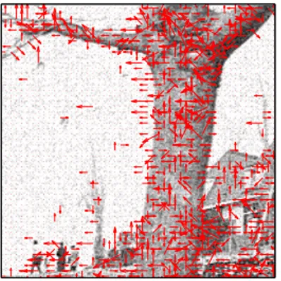
The motion field from t − 1 to t is represented by p0− p of all image positions p at time t. We can draw
the motion field between two frames by a vector graph, as shown in Figure2.2, where the direction and magnitude of each arrow correspond to the direction and magnitude of the motion at the pixel where the arrow takes its origin.
2. 3 Characterization of the motion
Before discussing in more details motion estimation techniques, the notion of motion should be clari-fied in the framework of image sequence processing. The four types of motion have been described in the subsequent sub-sections.
2. 3. 1 Pan motion
This type of motion occurs when the object in a video sequence moves linearly from the left direction to right or vice versa. The motion in the video can also be as a result of the movement of the camera instead of the object (in similar directions). When such a motion occurs in a video, the estimated motion should
be largely in a horizontal direction with relatively low or no motion detection in the vertical direction (a rotational movement of the camera about the vertical axis) as shown in Figure2.3.
2. 3. 2 Tilt motion
Tilt motion implies the movement of an object in the vertical direction. This means that the object in the video sequence moves either upwards or downwards. As in the previous case on pan motion, this motion can be a result of the camera movement as well. Consequently, when a motion estimation algorithm is applied to such a video sequence, the results should be concentrated in the vertical direction as compared to the horizontal direction (a rotational movement of the camera about the horizontal axis) as shown in Figure2.3.
2. 3. 3 Rotary motion
Rotary motion indicates the motion of an object around a horizontal or vertical axis in a video sequence. Since an object moving in a rotary motion has a constant axis, the results obtained from such a data set are usually concentrated on the edges of the moving object. This is true especially in cases when the moving object has a smooth surface or a constant color. In cases of irregular colored objects, the motion results could be concentrated over the whole object.
Further, it should be noted that the objects in a video sequence can move in a combination of these motions. In such cases, the estimated motion is a resultant of the individual motion results.
2. 3. 4 Zoom motion
Zoom motion can be of two types: Zoom-in and Zoom-out. As the name suggests, zooming in occurs when an object in a video sequence in concentrated upon. In the subsequent frames of a video sequence, the object of interest increases or enlarges in size. In most of the cases, the other objects in the frame tend to move out in the next frame. Motion detection for zoom in cases results in estimation of motion over the whole frame. This is because the camera moves all over the frame while trying to zoom in onto one object. Further, the results should be concentrated towards the center of the frame indicating the zooming in motion. On the other hand, zoom out motion results in lesser concentration on objects of interest. Zoom out leads to a decrease in size of objects in the succeeding frames. This may lead to insertion of more objects as the camera zooms out. Evidently, the results obtained for such a motion should be spread over the whole frame, with the vectors moving away from the center of the frame indicating zooming out motion of the camera.
Zoom-in and zoom-out motions can also be emulated if the object of interest moves closer or away respectively, from the camera while the camera focus remains the same.
Figure 2.3 – Typical types of camera motion.
2. 4 Motion models
The computation of motion is an ill-posed inverse problem [Efs91]. That is, (a) there is no solution for the data containing occlusion areas, (b) the solution satisfying the observed data is not unique, (c) there is a lack of continuity between data and solution since a slight modification of some intensity structures may cause significant change in the computation of the displacement vector, (d) on top of this, noise impedes the task of estimating motion. In order to describe the motion, all motion estimation techniques rely on the definition of a motion model. Generally, motion models can be classified as one of three types [BAHH92]: (a) fully parametric, (b) quasi-parametric and (c) non-parametric. Fully parametric models describe the motion of individual pixels within a region in terms of a parametric form. These include affine flow fields; planar surface motion under perspective projection models; and rigid body models. The advantage of the approach is that since all the pixels within the region of support can contribute to the motion estimation, robustness and high accuracy can be expected. On the other hand, when using non-parametric models some type of smoothness or uniformity constraint is imposed on the local variation of motion. As it might be expected, the results are limited in accuracy, but the model is applicable to a wide range of situations, as one motion vector is estimated per each pixel and therefore no hypothesis is made that those pixels belong to a common moving entity. A hybrid of the two model types is sometimes considered, leading to a quasi-parametric models, which represents the motion by a set of parameters as well as a local motion field.
In the remainder of this Section, different parametric motion models are derived by the projection of the 3-D motion in the scene onto the image plane. Furthermore, the 3-D motion can be described by a rigid body motion model. Consequently, a representation of the 2-D motion in the image plane is derived by the projection of this 3-D motion. For this purpose, a perspective or an orthographic projection is commonly
used. Finally, the restriction of the scene model to a patchwork of planar surfaces is assumed to avoid the estimation of the depth map. The latter hypothesis leads to fully parametric motion models.
2. 4. 1 Rigid body motion
The relation defining the 2-D motion in the image plane induced by the 3-D motion in the scene is derived as follows.
If we assume that a camera is represented by a pinhole, an image is formed by a perspective projection of the real world scene. Let R = (X, Y, Z)T be the Cartesian coordinates system fixed with respect to the camera,
and (x, y)T be the coordinates in the image plane (i.e. Z is perpendicular to the image plane and defines the optical axis). Under a perspective projection, r is related to R by:
x = X
Z and y =
Y
Z (2.3)
where the focal length has been normalized to 1 without any loss of generality.
In the formulation in terms of displacements, the 3-D rigid body motion equation is written as [Tsa02]:
− →
˙
R =−→R Ω +−→D (2.4)
where −→R and˙ −→R are the positions at time t and t − 1 respectively, Ω denotes the rotation matrix and D = (Dx, Dy, Dz)T is the translational displacement. Therefore, Ω and−→D denote differences in orientation
and position over a time interval. By introducing (2.3) in (2.4), it follows that " dx dy # = x−Ωzy+Ωy+DxZ 1−Ωyx+Ωxy+DzZ Ωxx+y−Ωx+DyZ 1−Ωyx+Ωxy+DzZ (2.5)
where (dx, dy) is the displacement of a point from time t − 1 to t; Ω has been approximated, assuming small
rotation angles, by:
Ω = 1 −Ωz Ωy Ωz 1 −Ωx −Ωy Ωx 1
2. 4. 2 Planar surface motion
The dependency on the depth map Z in (2.5) poses a problem. Since the motion estimation is based on a sequence of 2-D images, the depth map is not known a-priori and must be estimated. Estimation of a depth map from a set of 2-D images is a difficult problem, and is usually computationally intensive. Moreover, any estimation is likely to be inaccurate, and that will inevitably affect the accuracy of the motion estimation. In order to overcome these problems, the model of the scene is restricted to a patchwork of planar surfaces
which can closely approximate 3-D rigid bodies. This simplification removes the depth map dependency in the motion model and leads to a fully parametric model. A planar surface is defined as [Tsa02]:
KxX + KyY + KzZ = 1 (2.6)
where (Kx, Ky, Kz) relate to the surface slant, tilt, and the distance of the plane from the origin of the chose
coordinate system (in this case, the camera origin).
for the formulation in terms of displacements, the introduction of (2.6) in (2.5) gives " dx dy # = " a1+a2x+a3y a7x+a8y+a9 a4+a5x+a6y a7x+a8y+a9 # (2.7) where a1= Ωy+ DxKz a4= −Ωx+ DyKz a7= −Ωy+ DzKx a2= 1 + DxKx a5= Ωz+ DyKx a8= Ωx+ DzKy a3= −Ωz+ DxKy a6= 1 + DyKy a9= 1 + DzKz
(2.7) is commonly referred to as the perspective model. It defines the displacement in the image plane due to a moving planar surface under perspective projection. Usually, the parameters are normalized by a9, leading to an eight parameters model.
For the formulation in terms of displacements, under the same hypothesis of orthographic projection, an affine model is obtained from a first order Taylor series expansion of (2.7), yielding
" dx dy # = " a1+ a2x + a3y a4+ a5x + a6y # (2.8)
It is useful to note that the affine model can equivalently be expressed in terms of a translation vector, two scaling factors, and two rotation angles.
The affine model can be further simplified. For instance, the simple and widely used translation model with 2 parameters results from setting a2 = a3= a5 = a6= 0
" dx dy # = " a1 a4 # (2.9)
Given the different motion models available, the choice of the most appropriate one remains an open question. Obviously, the answer depends strongly on the type of application. It is obvious that a more complex parametric model can represent more complex motions. Consequently, it allows the motion of a larger region of the image to be precisely described.
2. 5 Region of support for motion representation
The set of points (x, y) to which a spatial and temporal motion model applies is called region of support, denoted R. The selection of a motion model and region of support is one of the major factors determining
the precision of the resulting motion parameter estimates. Usually, for a given motion model, the smaller the region of support R, the better the approximation of motion. This is due to the fact that over a larger area motion may be more complicated and thus require a more complex model. For example, the translational model can fairly well describe motion of one car in a highway scene while this very model would be quite poor for the complete image. Typically, the region of support for a motion model belongs to one of the four types listed below.
1. Global motion (R = the whole image)
The most constrained, yet simplest case is global motion, i.e., motion such that all image points are displaced in a uniform manner [NL91]. The region of support for such models consists of the whole image R . The global motion is usually camera-induced, as is the case of a camera pan or zoom. It is the simplest case because the motion of all the image points can be described by a small set of parameters (e.g., affine) related to camera parameters. At the same time, this is the most constrained case, because very few parameters describe the motion of all image points; only simple motion fields can be represented in this manner. The global motion model has been extensively used in computer vision, but has only recently found applications in video coding. It has recently been adopted in phase II of the MPEG-4 standard [KD98]; in sequences with clear camera pan/zoom, substantial rate savings have been achieved compared to standard methods based solely on local block motion estimation. 2. Motion of individual image points (R = one pixel )
This model applies to a single image point position (x, y) [HS81]. Typically, the translational spa-tial model is used jointly with the linear. This pixel-based or dense motion representation is the least constrained one since at least two parameters describe movement of each image point, and thus at least 2 × C × L parameters are used to represent motion in an image, with C, L being the numbers of columns and lines in the image. Consequently, a very large number of motion fields can be repre-sented by all possible combinations of parameter values, but computational complexity is, in general, high. At the same time, the method is the most complex due to the number of parameters involved. Although, from a purely computational point of view, it may not be the most demanding technique, pixel-based motion estimation is definitely one of the most demanding approaches. Dense motion re-presentation has found applications in computer vision, e.g., for the recovery of 3-D structure, and in video processing.
3. Motion of blocks (R = rectangular block of pixels)
This motion model applies to a rectangular (or square) block of image points. In the simplest case the blocks are non-overlapping and their union covers the whole image. A spatially-translational and temporally-linear motion of a rectangular block of pixels has proved to be a very powerful model and is used today in all digital video compression standards, i.e., H.26x, and the MPEG fa-mily [MPE93, MPE96]. Although very successful in hardware implementations, due to its simplicity,
the translational model lacks precision for images with rotation, zoom, deformation, and is often re-placed by the affine model.
4. Motion of regions (R = irregularly-shaped region)
This model applies to all pixels in a region R of arbitrary shape. The reasoning is that for objects with sufficiently smooth 3-D surface and 3-D motion, the induced 2-D motion can be closely approximated by the affine model applied linearly over time to the image area arising from object projection. Thus, regions R are expected to correspond to object projections. This is the most advanced motion model that has found its way into standards; a square block divided into arbitrarily-shaped parts, each with independent translational motion, is used in the MPEG-4 standard.
2. 6 Interdependence of motion and image data
Since motion is estimated (and observed by the human eye) based on the variations of intensity and/or color, the assumed relationship between motion parameters and image intensity plays a very important role. The usual, and reasonable, assumption made is that image intensity remains constant along the motion tra-jectory, i.e., that objects do not change their brightness and color when they move. This assumption implies, among others, that any intensity change is due in motion, that scene illumination is constant. Although these constraints are almost never satisfied exactly, the constant intensity assumption approximately describes the dominant properties of natural image sequences, and motion estimation methods based on it usually work well.
Let S be a variable along a motion trajectory. Then, the constant intensity assumption translates into the following constraint equation
dft(x, y)
dS = 0 (2.10)
i.e., the directional derivative in the direction of motion is zero. By applying the Chain rule, the above equation can be written as the well known motion constraint equation [HS81]
∂ft(x, y) ∂x v1+ ∂ft(x, y) ∂y v2+ ∂ft(x, y) ∂t = ( − → ∇ft(x, y))Tv +∂ft(x, y) ∂t = 0 (2.11)
where−→∇ = (∂x∂ ,∂y∂)T denotes the spatial gradient and v = (v
1, v2)T is the velocity to be estimated. The above constraint equation, whether in the above continuous form or as a discrete approximation, has recently served as the basis for many motion estimation algorithms. Note that, (2.11) applied at single position (x, y) is underconstrained (one equation, two unknowns) and allows to determine the component of velocity v in the direction of the image gradient−→∇ft(x, y) only. Thus, additional constraints are needed in order to uniquely solve for v [HS81]. Also, (2.11) does not hold exactly for real images and usually a minimization of a function of (−→∇ft(x, y))Tv + ∂ft∂t(x,y) is performed.
Since color is a very important attribute of images, a possible extension of the above model would be in include chromatic image components into the constraint equation. Let ft(x, y) = (f1, ..., fm)T be a
vector of attributes associated with an image; for example, its luminance and two chrominances as defined in the ITU-R 601 recommendation. Then, the constant intensity and constant color constraints can be written jointly in a vector form as follows:
∂ft(x, y) ∂x v1+ ∂ft(x, y) ∂y v2+ ∂ft(x, y) ∂t = − → 0 (2.12)
In general, estimates obtained using this constraint is more reliable than those calculated using (2.11) due to the additional information exploited. However, although (2.12) is a vector equation, different components of ft(x, y) may be closely related and therefore additional constraints may be needed.
The constraints discussed above find different applications in practice. A discrete version of the constant intensity constraint (2.11) is often applied in video compression since it yields small motion compensa-ted prediction error. Although motion can be compucompensa-ted also based on color using a vector equivalent of (2.12), experience shows that the small gains achieved do not justify the substantial increase in complexity. However, motion estimation from color data is useful in video processing tasks (e.g., motion compensated filtering, resampling), where motion errors may result in visible distortions. Moreover, the multi-component (color) constraint is interesting for estimating motion from multiple data sources (e.g., range/intensity data).
2. 7 Estimation criteria
Various motion representations as well as the relationship between motion and images discussed in the previous Section can be used now to formulate an estimation criterion. There is no unique criterion for motion estimation, however. The difficulty in establishing a good criterion is primarily caused by the fact that motion in images is not directly observable and that particular dynamics of intensity in an image sequence may be induced by more than one motion. Another problem is that most of the models discussed above are far from ideal. For example, the constant intensity model expressed through the motion constraint (2.11) is under-constrained and, at the same time, is often violated due to factors such as noise, non-opaque surface reflections, occlusions, or spatio-temporally varying illumination. Therefore, all attempts to establish suitable criteria for motion estimation require further implicit or explicit modeling of the image sequence.
2. 7. 1 DFD-based criteria
An important class of criteria arising from die constant intensity assumption (2.10) aims at the minimi-zation of the following error
If R is a complete image, this error is called a DFD. However, when R is a block or an arbitrarily shaped region, the corresponding error is called a displaced block difference or a displaced region difference. As before, subscripts may be omitted when the notation is clear from the context.
Motion fields calculated solely by minimization of the magnitude of die prediction error (2.13) are, in general, highly sensitive to noise if the number of pixels in the region of support R is not large compared to the number of motion parameters estimated, or if the region is poorly textured. However, such a minimization may yield good estimates for parametric motion models with few parameters and a reasonable region size.
To measure the magnitude of the prediction error ε(x, y) (2.13), a common choice is an Lp norm. For
the L2norm, this corresponds to the MSE:
M SE(dx, dy) =
X (x,y)∈R
(ft(x, y) − ft−1(x − dx, y − dy))2 (2.14)
This criterion, although very often used, is unreliable in the presence of outliers; even for a single large error
ε(x, y), ε2(x, y) is very large and by over-contributing to J1 it biases the estimate of (dx, dy). Therefore, a
more robust mean absolute error (MAE) criterion
M AE(dx, dy) =
X (x,y)∈R
|ft(x, y) − ft−1(x − dx, y − dy)| (2.15)
is the criterion of choice in practical video coders today. This criterion is less sensitive to bias due to the piecewise linear dependence of J2 on ε(x, y) and, at the same time, is less involved computationally. Also, the median-squared error (MDSE) criterion
M DSE(dx, dy) = med(x,y)∈R(ft(x, y) − ft−1(x − dx, y − dy))2 (2.16)
due to the use of a median operator, and a criterion based on the (differentiable) Lorentzian function
J(dx, dy) =
X (x,y)∈R
log(1 + (ft(x, y) − ft−1(x − dx, y − dy))2/2σ2) (2.17)
due to the saturation of the error function for outliers (σ is a scale parameter), perform well but require more computations. For a detailed discussion of robust estimation criteria in the context of motion estimation the reader is referred to the literature (e.g., [Bla92] and references therein).
2. 7. 2 Frequency domain criteria
Another class of criteria for motion estimation uses transforms, such as the Fourier transform F. Let
Ft(ux, uy) = F[ft(x, y)] be a spatial 2-D Fourier transform of the image ft(x, y), where (ux, uy) is a 2-D
that ft(x, y) = ft−1(x − dx, y − dy). This means that only translational global motion exists in the image
and all boundary effects are neglected. Then, by the shift property of the Fourier transform
F[ft−1(x − dx, y − dy)] = Ft−1(ux, uy)e−j2π(uxdx+uydy) (2.18)
Since the amplitudes of both Fourier transforms are independent of (dx, dy) while the argument difference
arg{F[ft(x, y)]} − arg{F[ft−1(x, y)]} = −2π(uxdx+ uydy) (2.19)
depends linearly on (dx, dy), the global motion can be recovered by evaluating the phase difference over a
number of frequencies and solving the resulting over-constrained system of linear equations. In practice, this method will work only for single objects moving across a uniform background. Moreover, the positions of image points to which the estimated displacement (dx, dy) applies are not known; this assignment must be
performed in some other way. Also, care must be taken of the non-uniqueness of the Fourier phase function which is periodic.
A Fourier-domain representation is particularly interesting for the cross-correlation criterion. Based on the Fourier transform properties and under the assumption that the intensity function ft(x, y) is real-valued,
it is easy to show that:
F[X
x
X
y
ft(x, y)ft−1(x − dx, y − dy)] = ˆft(ux, uy) ˆf∗t−1(ux, uy) (2.20)
where the transform is applied in spatial coordinates only and f∗ is the complex conjugate of f . This
equation expresses spatial cross-correlation in the Fourier domain, where it can be efficiently evaluated using the discrete Fourier transform (DFT).
2. 7. 3 Bayesian criteria
Bayesian criteria form a very powerful probabilistic alternative to the deterministic criteria described thus far [KD92]. If motion field (dt,x, dt,y) is a realization of a vector random field (Dt,x, Dt,y) with a given
a priori probability distribution, and image ft(x, y) is a realization of a scalar random field Ft(x, y) , then the maximum a posteriori (MAP) probability estimate of (dt,x, dt,y) can be computed as follows [KD92]:
( ˆdt,x, ˆdt,y) = arg max
(dx,dy)
P [(Dt,x, Dt,y) = (dt,x, dt,y)|Ft(x, y) = ft(x, y); ft−1(x, y)]
= arg max (dx,dy)
P [Ft(x, y) = ft(x, y)|(Dt,x, Dt,y) = (dt,x, dt,y); ft−1(x, y)]
In this notation, the semicolon indicates that subsequent variables are only deterministic parameters. The first (conditional) probability distribution denotes the likelihood of image ft(x, y) given displacement field
(dt,x, dt,y) and the previous image ft−1(x, y) , and therefore is closely related to the observation model.
In other words, this term quantifies how well a motion field (dt,x, dt,y) explains change between the two images. The second probability P [(Dt,x, Dt,y) = (dt,x, dt,y); ft−1(x, y)] describes the prior knowledge
about the random field (Dt,x, Dt,y) , such as its spatial smoothness, and therefore can be thought of as a motion model. By maximizing the product of the likelihood and the prior probabilities one attempts to strike a balance between motion fields that give a small prediction error and those that are smooth.
2. 8 A review of motion estimation techniques
A number of very different motion estimation algorithms have been proposed in the literature. Detai-led reviews are given by Musmann et al [MPG85], Nagel [Nag87], Aggarwal and Nandhakumar [AN88], Singh [Sin91], Sezan and Lagendijk [SL93], Barron et al [BFB94], and Tziritas and Labit [TL94]. These algorithms have been developed for very different applications such as image sequence analysis, machine vision, robotics, image sequence restoration or image sequence coding.
These techniques can be classified into the following categories:
1. Gradient techniques are based on the hypothesis that the image luminance is invariant along mo-tion trajectories. They solve an optical flow constraint equamo-tion which leads in a dense momo-tion field [BFB94].
2. Pel-recursive techniques can be considered as a subset of gradient techniques in which the spatio-temporal constraint is minimized recursively [NR79].
3. Black matching techniques are based on the matching of blocks between two images, which goal is to minimize a disparity measure [MPG85].
4. Frequency domain techniques are based on the use of frequency and phase information by means of tools like the Fourier transform to estimate the optical flow [PHGK77].
These techniques have been discussed in detail in the subsequent sub-sections.
2. 8. 1 Gradient techniques
Gradient techniques rely on the hypothesis that the image luminance is invariant along motion trajecto-ries. The Taylor series expansion of the right hand side in (2.1) gives
where−→∇ is the gradient operator. Neglecting the higher order terms (first order approximation), assuming
the limit ∆t → 0 , and defining motion vector −→v = (vx, vy)T =−→d /∆t we obtain
− →v .−→∇f
t(x, y) +
∂ft(x, y)
∂t = 0 (2.23)
The latter equation is known as the spatio-temporal constraint equation or the optical flow constraint equa-tion [HS81].
As the image intensity change at a point due to motion gives only one constraint (2.23), while the motion vector at the same point has two components, the motion field (actually the optical flow) cannot be computed without an additional constraint. In fact, only the projection of −→v on−→∇ft(x, y), in other words
the component of −→v parallel to the intensity gradient, can be determined from (2.23). This problem is known as the aperture problem. Therefore an additional constraint must be introduced to regularize the ill-posed problem and to solve the optical flow.
In [HS81], Horn ans Schunck introduce a smoothness constraint, that is to minimize the square of the optical flow gradient magnitude
(∂vx ∂x) 2+ (∂vx ∂y) 2 and (∂vy ∂x) 2+ (∂vy ∂y) 2 (2.24)
Consequently, the optical flow is obtained by minimizing the following error term Z Z {(−→v .−→∇ft(x, y) + ∂ft(x, y) ∂t ) 2+ α2[(∂vx ∂x) 2+ (∂vx ∂y ) 2+ (∂vy ∂x) 2+ (∂vy ∂y) 2]}dxdy (2.25) where α2 is a weighting factor. This minimization problem is solved by the variational calculus and an iterative Gauss-Seidel procedure.
Many variations of the above algorithm have been proposed. A method that imposes a local smoothness constraint on the motion field was proposed by Lucas and Kanade [LK81]. They made the assumption that the optical flow estimation can be viewed as being constant over small local image regions (typically 5 × 5 pixels). This was expressed as the minimization of the integral
Z Z
ω(x, y)2(−→v .−→∇ft(x, y) + ∂ft(x, y)
∂t )
2dxdy (2.26)
where ω(x, y) denotes a suitable isotropic window function accentuating the center part of the local re-gion. From the integral above an expression for the motion field was derived using standard least squares techniques.
More sophisticated smoothness constraints have been proposed that alleviates some of these shortco-mings. A generalization of the Horn and Schunck method was proposed by Nagel [Nag83, Nag87], making use of a directionally sensitive smoothness constraint to better cope with discontinuities. The second term in the integral (2.25), ie the spatial smoothness constraint, was replaced by a term representing the square of the projection of the optical flow vector onto the direction perpendicular to the gradient. This formulation