Fiscal Interaction in Canada: The Case of Personal Income Taxes par
Maria Silvia de Moraes Barros
Travail dirigé par Prof. François Vaillancourt
Université de Montréal
Département de Sciences Économiques Faculté des Arts et Sciences
CONTENTS
LIST OF TABLES AND FIGURES... iii
INTRODUCTION...1
SECTION I. - LITERATURE REVIEW...2
1.1 Theoretical Model ...2
1.1.1 Vertical Externalities ...2
1.1.2 Literature Review of Empirical Studies ...4
1.1.3 Equalization Grants...5
1.2 Literature Review of Empirical Studies ...7
SECTION II. - Data and Model...11
2.1 Effective Provincial Personal Income Tax Rates ...12
2.2 Effective Federal Personal Income Tax Rates...14
2.3 Competing Provincial Effective Personal Income Tax Rates ...16
2.4 Equalization Grants...20
2.5 Control Variables...21
SECTION III.- Econometric Issues and Results...24
3.1 Unit root and cointegration tests ...24
3.2 Fixed vs. Random effects model, heteroskedasticity, contemporaneous and serial correlation test...30 3.3 Endogeneity ...32 3.4 Regression Results ...33 3.4.1 Vertical Tax Interaction and Vertical Externalities ...35
3.4.2 Horizontal Tax Interaction and Horizontal Externalities...36
3.4.3 Equalization Grants...36
3.4.2 Control Variables...37
CONCLUSIONS ...38
LIST OF TABLES AND FIGURES
Figure 1: Effective Provincial Personal Income Tax Rates - Eastern Canadian Provinces (1981-2004)
Figure 2 - Effective Provincial Personal Income Tax Rates - Western Canadian Provinces (1981-2004)
Figure 3 - Effective Federal Personal Income Tax Rates - Eastern Canadian Provinces (1981-2004)
Figure 4 - Effective Federal Personal Income Tax Rates -Western Canadian Provinces (1981-2004)
Figure 5 - Effective Competing Personal Income Tax Rates- criterion 1 - Eastern Canadian Provinces (1981-2004)
Figure 6: Effective Competing Personal Income Tax Rates- criterion 1 - Western Canadian Provinces (1981-2004)
Figure 7: Effective Competing Personal Income Tax Rates- criterion 2 - Eastern Canadian Provinces (1981-2004)
Figure 8: Effective Competing Personal Income Tax Rates- criterion 2 - Western Canadian Provinces (1981-2004)
Table 1: Literature Review Summary of Empirical Studies Table 2: Data description and source
Table 3: Summary Statistics
Table 4: Unit Root Tests Results (level form) Table 5: Unit Root Tests Results (logarithmic form) Table 6: Unit Root Tests Results (first difference form)
INTRODUCTION
As federal countries are composed of at least two levels of government, the interactions between federal and subnational governments can be the subject of economic analysis. An important and well studied issue relating to federal governments is fiscal federalism and the possible externalities caused by the existence of federal and subnational taxation of the same tax base. The consequences of the existence of fiscal federalism can be both beneficial and inefficient. These inefficiencies are found, for example, in the form of horizontal externalities (tax competition) and vertical externalities.
Several empirical studies have examined these possible inefficiencies: in the United States such as Besely and Rosen (1998) on the taxation of gasoline and cigarettes, in Canada such as Hayashi and Boadway (2001) on the taxation of corporate income and Esteller-Moré and Solé-Ollé (2002) on the taxation of personal income, and in the OCDE countries such as Goodspeed (2000) on the taxation of personal income.
The main goal of this research paper is to empirically determine the interactions that may exist between the taxation of personal income in Canada by both the provincial and the federal levels of government for the 1981-2004 period. By doing so, it will be possible to analyse the existence of vertical and horizontal externalities as a result of taxation of the same tax base by those two levels of government. In other words, the main question is: how do provinces respond to a federal and other provincial tax rate modifications?
This research paper is divided in three sections: The first is the literature review of studies on fiscal federalism .In this section we describe the theoretical background supporting the model we develop and empirically estimates. The second is a description of the data and the variables used to estimate the model. The third is the results of the unit root and cointegration tests, as well as the results of our estimations. We end with the conclusion and potential extensions of this research.
SECTION I. - LITERATURE REVIEW
1.1 Theoretical Model
As labour is a potentially mobile resource, the fiscal policies of governments may affect the decision of an individual to move from one jurisdiction to another jurisdiction where the available set of public goods and taxes would increase the individual’s utility. The mobility of labour can induce individuals with similar preferences to congregate together in localities, however, some inefficiencies may arise as a consequence of decentralized decisions. The different choices made by local governments regarding taxation and the provision of public goods can induce fiscal externalities, causing an inefficient allocation of labour across jurisdiction (Boadway, Wildasin, 1984). These fiscal externalities can be both vertical and horizontal.
1.1.1 Vertical Externalities
The theoretical model that is the basis of our empirical study is the one described by Esteller-Moré and Solé- Ollé (2002). It is assumed that each subnational unit will maximise the indirect utility function of a representative household (taxpayer) subject to its budget constraint. As considered in most of the theoretical literature on fiscal interaction, the provinces behave as Nash, implying that a province will take as given the federal government’s tax rates. Thus, the provincial government will maximise the indirect utility function given by the net wage rate
( )
wnv and the utility given by the federal and provincial level of public goods (h
( ) ( )
g ,H G ,The result of the first order condition of the utility maximisation is that the marginal benefit of public goods equals the marginal cost of public funds:
⎟ ⎠ ⎞ ⎜ ⎝ ⎛ − = l l t h ' 1 1 ' or MB=MCPF.
One should note that the provincial tax rates appear only in the calculation of the marginal cost of public funds, as the provincial tax setting function can be written as t= f
(
T,w,Rexog))
.In thiscase, the province is neglecting the federal tax rate and by doing so, underestimating the marginal cost of taxation and consequently sets a higher tax rate with respect to what would be socially efficient.
Also, from the maximisation problem, it is possible to set the provincial tax rate as a function of the federal tax rate, the gross wage rate, and other exogenous revenues the province receives. The vertical externality comes from the fact that ∂t/∂T ≠ 0. The sign of this vertical interaction can be positive or negative. Facing an increase in the federal tax rate, the province can either increase or decrease its own tax rate, on the effect on the marginal benefit of public goods and on marginal cost of public funds. In other words, from the point of view of the marginal benefit of public goods, if the federal tax rate increases, the revenue of provinces decreases and so to offer the same level of public goods as before, the province will have to increase its tax rate and thus the expected sign of the interaction is positive. From the point of view of the marginal cost of public funds, however, the effect on the provincial tax rate is ambiguous. Since an increase in the federal tax rate results in a smaller tax base either through the departure of individuals to other tax authorities or through an increase in tax evasion, the marginal cost of public funds is necessarily affected. This effect may be positive or negative. Should the marginal cost of public funds increases due to the departure of high income individuals or greater tax evasion, an increase of the provincial tax rate would be necessary to obtain the required revenues and compensate for the higher marginal cost. However, if the marginal cost of public funds decreases through a departure of lower income, the effect on the provincial tax rate is negative.
1.1.2 Horizontal Externalities
The horizontal tax externality, on the other hand, exists as a consequence of possible tax competition between provinces. As we are dealing with income taxation, the problem appears because labour should be considered as a mobile factor. As provinces know they can loose a part of their tax base as a consequence of migration, it is assumed that the provincial governments are in a ‘prisoner’s dilemma’ .This consideration leads us to the result that a given province will set its tax rate too low and leading to inefficiency. The maximisation problem here is analogous to the one described for the vertical externality problem and is also based on Esteller-Moré and Solé- Ollé (2002). The difference is that now labour is a mobile factor and we take into consideration the migration function of mobile taxpayers living in a given province. The group of mobile labours will choose where to live when the wage rate equals to the marginal productivity of labour: j i T t f T t fi'(1− i − )= j'(1− j − ),∀ ≠ ,
The migration function is a function of its own provincial tax rate, the other provincial tax rate, and the federal tax rate. The problem can be written as:
( ) ( )
( )
[
v ki h g H G]
t
+ +
max
, subject to gp =i t⋅(
wini +kipi)
⋅l+Rexog and ni = f(ti,t−i;,T) Where:i
l = labour supply.
The first order condition is also MCPF = MB or
⎥ ⎥ ⎦ ⎤ ⎢ ⎢ ⎣ ⎡ ⎟⎟ ⎠ ⎞ ⎜⎜ ⎝ ⎛ + ∂ ∂ + + = ' '' ' ' ' 1 1 1 1 i i i i i i i im i i i f f n n t t n f p f n h
So, the provincial tax rate is a function of the other provinces’ tax rates, the federal tax rate, the number of immobile tax payers and mobile taxpayers, and other exogenous revenues.
If a province decreases its tax rates, the number of people migrating out of it will also decrease and may even be replaced by in-migration, but if the other provinces tax rates decrease, the number of people migrating out will increase. The impact of a change in the federal tax rate on migration is ambiguous. The first order condition of the maximisation problem gives us the provincial tax setting function. The provincial tax rate is now function of the federal tax rate, the other provincial tax rates, the population of each province, the number of immobile labour within the province and the other exogenous revenues. The tax interaction has an ambiguous effect. In the model described, if province j increases its tax rate, this will cause an increase in its revenue and this will also increase the revenue of province i as a consequence of the inflow of tax base. The marginal benefit of public goods decreases and province i will, in response to this fact, decrease its own tax rate. The sign of the effect on the marginal cost of public funds is, however, ambiguous as in the case of vertical interactions. Again, the sign of the interaction that may exist between the different provincial tax rates is determined empirically.
1.1.3 Equalization Grants
Finally, as one of the characteristics of Canada is the existence of equalization grants, it is interesting to analyse how the presence of this particularity affects the setting of provincial tax rates. “The transfer is calculated as the difference between the amount of revenue that would be
raised per capita by applying a national average provincial tax rate to a standard set of national tax bases and the amount that would be raised by applying the same national average tax rate to a recipient province’s own tax bases” (Hayashi and Boadway, 2001, p.482). Also, “in federal
systems, intergovernmental transfer programs are frequently designed and implemented to serve regional equity objectives and promote efficient tax and fiscal policies for subnational governments” (Smart, 1998, p.189). They also point that the existence of equalization grants may
lead to distortionary tax policies. This distortion takes the form of a province setting tax rates too high. “To the extent that local tax bases are elastic with respect to distortionary tax rates,
provinces can induce larger equalization transfers by increasing tax rate” (Smart 1998, p. 190).
The argument for this distortion is that as tax rates increase, the tax bases decrease (as economic activities may shift to other provinces), leading to an increase in equalization entitlement. “Thus
the grants in effect compensate for a portion of the marginal deadweight loss of tax increases”
1.2 Literature Review of Empirical Studies
As mentioned in the last section, the first source of tax interaction arises from vertical externalities. As pointed by Esteller-Moré and Solé-Ollé (2001), vertical externalities in the design of tax policy arise mainly as a result of concurrent taxation. This means that both federal and local governments have the power to tax the same tax base.
Empirical studies such as Besley and Rosen (1998) on the taxation of gasoline and cigarettes in the United States find a positive relationship between local and federal taxation. Goodspeed (2000) in analyzing the taxation of personal income in the OCDE countries finds that when federal governments increase personal income taxes, subnational governments’ tax rates respond negatively. Boadway and Hayashi (2000) find that provincial tax rates have a negative response to the federal tax rate in the case of corporate tax in Canada. Esteller-Moré and Solé-Ollé (2001) find a positive relation between the changes in the federal rate and state rates for both the taxation of personal income and general sales in the United States. They find also in another paper (Esteller-Moré and Solé-Ollé (2002)) that the federal personal income tax rate has a positive effect on provincial personal income tax rates in Canada.
The second important source of inefficiencies is the horizontal externality arising from tax competition. What would be the consequence for Quebec tax rates, for example, if tax rates increase in Ontario? This horizontal tax interaction also has a theoretically ambiguous effect. As in the case of vertical externalities, we can only determine the impact of changes in competing tax rates on provincial tax rates empirically. Several empirical studies find relevant interactions between the taxation by the same level of government. Boadway and Hayashi (2000), find that some provinces in Canada increase their corporate tax rates in response to increases in the tax rates of other provinces. Esteller-Moré and Solé-Ollé (2002) also find significant positive response of the provincial personal income tax rate to the personal income tax rate of competing provinces.
The third source of tax interaction that is relevant for this paper is the institutional framework. In the case of Canada, equalization grants are an important issue in studying tax interaction. Smart
(2007) find empirically for the period of 1972-2002 that Canadian provinces increase their tax rates in response to more generous to equalization transfers. Higher taxes can induce distorting local tax bases and thus increasing federal transfers. Esteller-Moré and Solé-Ollé (2002) report the same result concerning personal income tax rates in Canada, that is, the fact of receiving equalization payments leads to higher personal income tax rates.
Table 1 summarizes some of the empirical studies on the interaction between federal and local tax rates in the context of federal countries.
Table 1 - Literature Review Summary of Empirical Studies
Author and Year Subject Variables Year Population Estimation
Method Results
A Esteller-Moré, A
Solé-Ollé. (2002). Personal Income Taxation in Canada Dependent: effective provincial tax rate Independent: effective federal tax rate, effective competing provincial tax rates, equalization grants, and control variables( income, transfers, natural resources, population under 15 and over 65, unemployment rate and political environment) 1982-1996 The 10 Canadian provinces (150 observations) OLS with fixed effects and Instrumental Variables.
Evidence of tax interaction: positive reaction of provincial tax rates due to changes in federal tax rates, neighbouring provincial tax rates, and equalization grants.
A Esteller-Moré, A
Solé-Ollé. (2001). Personal Income Taxation in the US Dependent: effective provincial tax rate Independent: effective federal tax rate, effective competing state tax rates, reciprocal deductibility, and control variables (income, federal grants, population under 18 and over 65, political environment). 1987-1996 41 US States (410 observations) OLS with fixed effects and Instrumental Variables.
Evidence of tax interaction: positive reaction of state tax rates due to changes in federal tax rates and neighbouring states tax rates, and negative reaction of state tax rates due to reciprocal tax deductibility.
Besley, T.J.,
Rosen, H.S., 1998 Taxation of cigarette and gasoilne in the US (vertical
externality)
Dependent: state tax rate
Independent: federal tax rate, federal grants to the states, and control variables (macroeconomic environment – national unemployment rate, real GDP and state’s economic, demographic situation – state population, population density, state income, state unemployment rate, the proportion of individuals between 5 and 17, and the
1975-1989 Continental States of the United States (705 observations) OLS with a variant of the robust standard error procedure of White and Instrumental Variables.
Evidence of tax interaction: positive reaction of states tax rates due to changes in the federal tax rates.
proportion o f individuals over 65, political environment, and the importance of the tobacco and gasoline production.
Goodspeed, T. J.
(2000). Impact of horizontal and vertical
externalities on tax setting by local governments in a federation (the case of the OCDE countries)
Dependent: local income tax rate
Independent: national income tax rate, proportion of income of 20% poorest, and local revenue per capita.
1975-1984 ODCE countries (130 observations) Tobit and instrumental variables.
Evidences of the a negative reaction of local tax rates due to changes in the national income tax rates and lower poverty rate. Hayashi, M. and R. Boadway. (2001). Intergovernmental tax interaction (business income taxes in Canada)
Dependent: average provincial business income tax rates.
Independent: average federal business income tax rate, equalization grants, inflation, business cycle (GDP growth rates), interest rates, wages, political party in power, public sector deficits
1963-1996 The Federal Government and 10 Canadian Provinces (340 observations)
IFGLS Evidences of the existence of vertical and horizontal externalities in the setting of business income taxes by provinces. The response of provincial tax rates to changes in the federal tax rate is negative. The horizontal interaction is however, found to be positive.
Smart, M. (2007) Influence of equalization grants on subnational tax rates
Dependent: effective provincial tax rates Independent: population-weighted average of the same tax rates, indicator variable for equalization-receiving provinces, and control variables (GDP per capita, percentage of population under 19, percentage of population over 64, political party)
1972-2002 (excluding 1973 and 1982) The 10 Canadian Provinces (190 observations) OLS and instrumental variables
Evidences of the existence of a positive reaction of provincial tax rates in the presence equalization grants.
SECTION II. – Data and Model
In Canada, the main source of revenue for the federal government and provincial governments comes from the taxation of personal income. In 2004, 20.7% of total federal revenue came from the taxation of personal revenue while for provinces on average it accounted for 17.63%1 . The period studied is 1981-2004, constrained by the data from Table 384-0004 (CANSIM, Statistics Canada). We thus update the results found in other empirical studies for Canada (1982-1996). The model to be estimated includes variables suggested by our review of the theoretical and empirical studies. Thus, we estimate a model that tests the existence of vertical externalities and horizontal externalities, as well as the influence of the institutional framework in Canada by taking into account the existence of equalization grants.
Table 2 describes all the data considered and their sources.
Table 2: Data, Description, and Source
Variable Description Source
Effective Provincial tax rates (dependent)
ratio provincial income tax revenue/provincial personal income
Table 384-0004 and table 384-0001 (CANSIM, Statistics Canada)
Effective Federal tax rates (independent)
Ratio federal income tax revenue /provincial personal income component
Table 384-0004 and table 384-0001 (CANSIM, Statistics Canada)
Equalization (independent) Dummy variable (1 if the province is a equalization recipient and 0 if it is not)
Finances of the Nation: transfers payments (Canadian Tax Foundation)
Per capita Personal income (independent)
Per capita income Table 384-0004 and table 051-0001 (CANSIM, Statistics Canada)
Per capita transfers (independent)
Per capita transfers from federal government to provinces
Table 384-0004 and table 051-0001 (CANSIM, Statistics Canada)
% Population under 15 (independent)
Percentage of the population under 15 years old in the province
Table 051-0001 (CANSIM, Statistics Canada) % Population over 65
(independent)
Percentage of the population under 65 years old in the province
Table 051-0001 (CANSIM, Statistics Canada) Unemployment rate
(independent)
Percentage of the labour force unemployed
Table 282-0002 (CANSIM, Statistics Canada)
2.1 Effective Provincial Personal Income Tax Rates
The provincial tax rates are the dependent variable, as we study the reactions of provinces to changes in the federal tax rates and other provinces tax rates. The effective provincial tax rate is defined as the ratio of total provincial income tax received and the total provincial personal income (see Table 2). This gives an average tax rate, which is also used in Goodspeed (2000) and Hayashi and Boadway (2001). The effective tax rate is used as the statutory tax rates personal income in Canada are progressive and thus single marginal tax cannot be taken as representative for all (Esteller-Moré and Solé-Ollé, 2002) households. Another reason pointed by Esteller-Moré and Solé-Ollé (2002) is that “averages rates are often employed to represent interjurisdictional
differences in taxation” (p.18). Finally, the adoption of a provincial tax-on-income ( taxes levied
based on federally-defined taxable income) structure for individuals replacing the tax-on-tax (taxes levied as a percentage of federal income tax) by nine of the ten provinces (Quebec already used this approach) in 2000 and 2001 makes more difficult the analysis of the changes in statutory tax rates. Nova-Scotia, New Brunswick, Ontario, Manitoba, and British Columbia adopted the change in 2001, while Newfoundland, Prince Edward Island, Saskatchewan, and Alberta implemented the tax-on-income structure in 2001.2 Thus, to test the possible interactions that may exist between federal and provincial taxation, effective rates are used instead of statutory rates3. Figure 1 and 2 show us the evolution of the effective provincial tax rates.
Figure 1 - Effective Provincial Personal Income Tax Rates - Eastern Canadian Provinces (1981-2004) 4,00% 6,00% 8,00% 10,00% 12,00% Year 1982 1984 1986 1988 1990 1992 1994 1996 1998 2000 2002 Year
New foundland and Labrador Prince Edw ard Island Nova Scotia New Brunsw ick Quebec
Source: Statistics Canada, CANSIM, Provincial economic accounts
Figure 2 - Effective Provincial Personal Income Tax Rates - Western Canadian Provinces (1981-2004) 3,00% 4,00% 5,00% 6,00% 7,00% 8,00% 9,00% 1981 1983 1985 1987 1989 1991 1993 1995 1997 1999 2001 2003 Year Ta x r a te s
Ontario Manitoba Saskatchew an Alberta British Columbia
Although the province of Quebec has an abatement provided under the federal-provincial arrangement of 16.5% that is corrected for calculating its provincial income tax, its tax rates are the highest for all the periods considered. This difference may exist as a consequence of different laws concerning the taxation of personal income in Quebec and the federal government, while the other provinces follow the same rules as the federal government in defining taxable income. The lowest personal income tax rate is the one from Alberta, for all the period considered. The periods of 1985-1987 and 1993-1997 show a trend of increasing tax rates for all provinces.
It should be noted that from 1999, most provinces had a decrease in their tax rates, except for Nova Scotia, Quebec, and Manitoba. In 2000, this decrease continues and more intensely, with the exception of Ontario. This year, as shown in the publication ‘Finances of the Nation’, all provinces had cut personal income tax rates, as a consequence of changes in the tax structure. During this year, all provinces announced their adoption of a provincial tax-on-income structure for individuals in either 2000 or 2001(Quebec already used this system).
2.2 Effective Federal Personal Income Tax Rates
The second variable used is the independent variable federal tax rate. This variable will be important in analysing vertical externalities. For the same reason aforementioned for the provincial tax rates, here we use the effective federal tax rate, defined as the ratio of total federal income tax received and the total federal personal income. Figure 3 and 4 below show its evolution.
Figure 3 - Effective Federal Personal Income Tax Rates - Eastern Canadian Provinces(1981-2004) 7,00% 8,00% 9,00% 10,00% 11,00% 12,00% 13,00% 14,00% 1981 1983 1985 1987 1989 1991 1993 1995 1997 1999 2001 2003 Year
New foundland and Labrador Prince Edw ard Island Nova Scotia New Brunsw ick Quebec
Source: Statistics Canada, CANSIM, Provincial economic accounts
Figure 4 - Effective Federal Personal Income Tax Rates -Western Canadian Provinces(1981-2004) 8,00% 9,00% 10,00% 11,00% 12,00% 13,00% 14,00% 15,00% 16,00% 1981 1983 1985 1987 1989 1991 1993 1995 1997 1999 2001 2003 Year
Ontario Manitoba Saskatchew an Alberta British Columbia
The province of Ontario has, for the period considered, maintained itself as the province with the highest federal tax rate, while Quebec has the lowest federal personal income tax rate for the same period. The difference between the lowest and the highest tax rate is not higher than 3.8%.Ontario has a higher average tax rate since it has a higher per capita income. Combining this with the progressive taxation of income yields the higher average effective personal income tax rates for Ontario.
According to Wilson and Dungan (1992), the budget of 1983 was an attempt to combine near-term stimulus with tax structure changes in order to stimulate investments and reduce the deficit. So in the short term, the consequence was a decrease in federal tax rates until 1984 with subsequent increases in tax rates until 1987. Also, as described in the section ‘Federal Budgetary Outlook’ of the publication Finances of the Nations, the government had, in 1985, two main concerns, unemployment and deficit. The second goal was met trough expenditures reductions and tax increases. Federal income tax was subject to a temporary surtax during 1985 and to both a temporary and a general surtax in 1986, explaining the fast increase of federal tax rates in these two years.
One can also notice that starting from 2000 until 2003, there is a decrease in the federal tax rates. As mentioned in the publication ‘Finances of the Nation’, “Individual taxpayers received some
tax relief in this year’s budget because of the minister’s announcement of the resumption of full indexation of the federal system, effective for the 2000 and subsequent taxation years”. The
impacts of tax reduction became apparent in 2000 as is reported by the Department of Finance using the following measures: full indexation of the personal income tax system, reduction of the middle tax rate from 26% to 24%, elimination of 5% deficit reduction surtax on incomes up to about $85,000 and reduced for all others, and the increase of the maximum annual payments
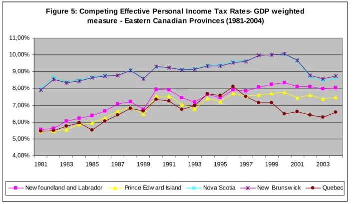
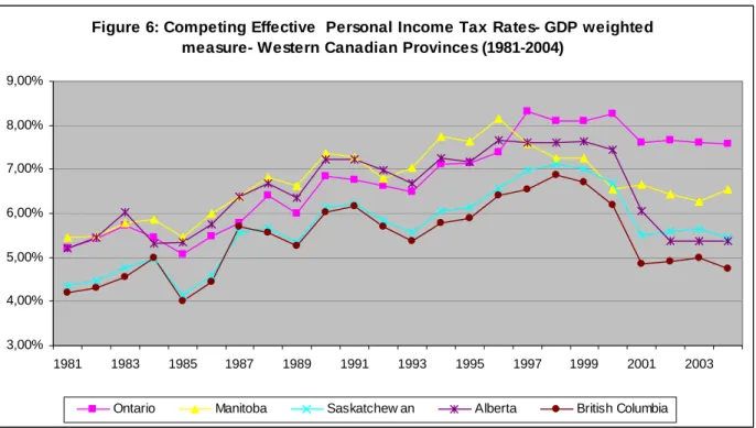
‘Competing provincial effective personal income tax rates’ is also used as an independent variable in the calculation of the competing tax rates, as one of the aims of this research is to evaluate if the personal income tax rates of competing provinces have influence the provincial tax rate (horizontal externality). To calculate the competing tax rate, we have to find a criterion on how provinces may affect one another, that is, a measure that represents the possible movement of personal income tax bases between provinces. Two methods were used, one based on the importance of the GDP of each province and another based on the distance and population. The first one is measured taking, for example, for the province i, all other provincial tax rates multiplied by the weight of each GDP in the national GDP.5
(
)
∑
∑
≠ ⎟⎟⎠ ⎞ ⎜⎜ ⎝ ⎛ × = j i J j j i PIB PIB t tThe evolution of the competing tax rates using this criterion is reported in Figure 5 and 6 that follows:
Figure 5: Competing Effective Personal Income Tax Rates- GDP weighted measure - Eastern Canadian Provinces (1981-2004)
4,00% 5,00% 6,00% 7,00% 8,00% 9,00% 10,00% 11,00% 1981 1983 1985 1987 1989 1991 1993 1995 1997 1999 2001 2003
New foundland and Labrador Prince Edw ard Island Nova Scotia New Brunsw ick Quebec
Source: Statistics Canada, CANSIM, Provincial economic accounts
Figure 6: Competing Effective Personal Income Tax Rates- GDP weighted measure- Western Canadian Provinces (1981-2004)
3,00% 4,00% 5,00% 6,00% 7,00% 8,00% 9,00% 1981 1983 1985 1987 1989 1991 1993 1995 1997 1999 2001 2003
Ontario Manitoba Saskatchew an Alberta British Columbia
Source: Statistics Canada, CANSIM, Provincial economic accounts
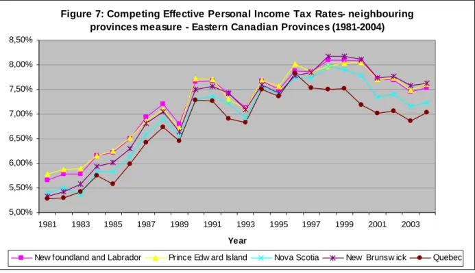
The second method for calculating the competing tax rates is the same as used by Esteller-Moré and Solé-Ollé (2002). They take contiguous provinces as being possible sources of immigration and migration and then weigh provincial tax rates by population and inverse distance between the main provincial centres (cities with biggest population in each province). This gives us the weight (
Ν
ij) for each province defined as6:Ν
ij=(
w
ij∑w
ij)
; wherew
ij =d
n
c
ij j ij× , andThe evolution of the competing tax rates is shown in figure 7 and 8.
Figure 7: Competing Effective Personal Income Tax Rates- neighbouring provinces measure - Eastern Canadian Provinces (1981-2004)
5,00% 5,50% 6,00% 6,50% 7,00% 7,50% 8,00% 8,50% 1981 1983 1985 1987 1989 1991 1993 1995 1997 1999 2001 2003 Year
New foundland and Labrador Prince Edw ard Island Nova Scotia New Brunsw ick Quebec
Source: Statistics Canada, CANSIM, Provincial economic accounts
Figure 8: Competing Effective Personal Income Tax Rates- neighbouring provinces measure - Western Canadian Provinces (1981-2004)
3,00% 4,00% 5,00% 6,00% 7,00% 8,00% 9,00% 10,00% 11,00% 1981 1983 1985 1987 1989 1991 1993 1995 1997 1999 2001 2003 year
Ontario Manitoba Saskatchew an Alberta British Columbia
The evolution of the competing tax rates shows us that the province of Ontario had the highest competing tax rates for the period considered. The reason for this is that Ontario is contiguous to the provinces of Quebec and Manitoba. As mentioned before, the province of Quebec has the highest provincial tax rates and thus influencing the calculation of its weight in contiguous provinces such as Ontario.
2.4 Equalization Grants
According to MacNevin (2004), the formal Canadian equalization system has its origin in 1957 and it is renewed every five years. Changes have occurred since then, but the most important one comes with the Constitutional Act. In 1982 the equalization was incorporated in the constitution, the five province standards for equalization was adopted, and a ceiling and floor were established for equalization entitlements. As also pointed by MacNevin (2004), “The equalization program
is the principal means of achieving horizontal fiscal balance within the Canadian federation; horizontal balance in this context relates to the distribution of fiscal resources among the provinces. This role makes equalization a key element in Canada’s system of federal-provincial fiscal arrangements” (p.1). The formula for the calculation of equalization payments is set by
federal legislation and depends on the fiscal capacity of each province evaluated with respect to an established standard. That way, provinces that do not meet the standard are eligible for equalization payments. Provincial fiscal capacity is assessed with the national average rate for each tax described in the ‘representative revenue system’ applied to the province’s estimated base for each tax. (MacNevin, 2004)
province of British Columbia was not a recipient until 2001 and the province of Saskatchewan was not a recipient for the period of 1982-1985. All other provinces were recipients of equalization grants during all the periods considered.
2.5 Control Variables
To account for the fact that the level of provincial income tax rates may also be affected by economic and social factors, we include control variables: personal income per capita8, transfers per capita to the provinces9, percentage of population over 65 years old10, percentage of population under 15 years old11, and unemployment rate12
2.5.1 Per capita income
The effect of a change in the per capita income on personal income tax rates is ambiguous. More personal income means more revenue for the government with the same tax rates, so it is not possible to determine the effect of the changes in income per capita in tax rates. Per capita income has trend of increase (in nominal terms) for all provinces. The province of Alberta presented the highest income per capita among all provinces and had remarkable growth starting in 1999. The province with the lowest income per capita is Newfoundland and Labrador, although this province also had increases in income per capita.
2.5.2 Per capita transfers
The provinces of Newfoundland and Labrador and Prince Edward Island received the most federal transfers per capita during the period studied. The provinces of Ontario, British Columbia, and Alberta received the least federal transfers. As the revenue of provinces increase as transfers increase, one might expect that the effect of the transfers per capita on provincial tax rates is expected to be negative.
8Statistics Canada CANSIM Table 384-0001 and CANSIM Table 051-0001. 9 Statistics Canada CANSIM Table 385-0002.
10 Statistics Canada, CANSIM, Table 051-0001. 11 Idem.
Combining the analysis of the income per capita with transfers per capita, it is possible to conclude that the richest provinces, the ones with higher income per capita were the ones that received the lowest federal transfers.
2.5.3 Percentage of population over 65 years old, percentage of population under 15 years old, and unemployment rate
These three control variables account for the possibility that “populations with higher shares of
potential users of public services and/or higher cost of delivering those services will need higher levels of expenditure and, therefore, will be burdened more heavily through income taxes” (A
Esteller-Moré, A Solé-Ollé., 2002, p.22). The percentage of the population over 65 years tends to increase in the period of study, while the percentage of the population under 15 tends to decrease. The unemployment rate is instable and oscillates between periods of increase and decrease.
The model to be estimated will be:
μ
λ
π
δ
β
α
it l ij l l ij ij ij i ijT
n
eq
Z
t
= + * + + * +∑
* + Where:i
= provincej
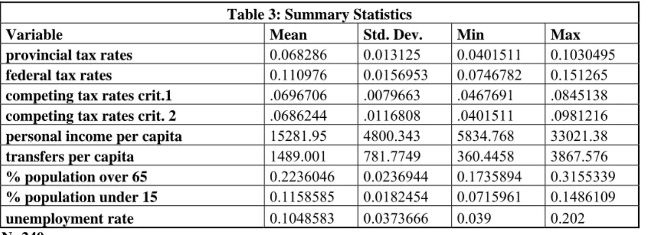
= timeTable 3 summarizes the data.
Table 3: Summary Statistics
Variable Mean Std. Dev. Min Max
provincial tax rates 0.068286 0.013125 0.0401511 0.1030495 federal tax rates 0.110976 0.0156953 0.0746782 0.151265 competing tax rates crit.1 .0696706 .0079663 .0467691 .0845138 competing tax rates crit. 2 .0686244 .0116808 .0401511 .0981216 personal income per capita 15281.95 4800.343 5834.768 33021.38 transfers per capita 1489.001 781.7749 360.4458 3867.576 % population over 65 0.2236046 0.0236944 0.1735894 0.3155339 % population under 15 0.1158585 0.0182454 0.0715961 0.1486109 unemployment rate 0.1048583 0.0373666 0.039 0.202 N=240
SECTION III.- Econometric Issues and Results
3.1 Unit root and cointegration tests
The estimation of a pooling cross-section time series data model data gives us some econometrics issues related to time series econometrics. As the data used is composed of ten provinces and 24 years, non-stationary series may exist and thus affecting the estimation of the model. This non-stationarity can lead us to a spurious regression, whereby two time series appears to be related when they are not. The two unit root tests used are the ones based on the methods described by Levin, Lin and Chu (2000) and Im et al. (2003) (to simplify the notation, the Levin, Lin and Chu test and Im et al test will be called LL and IPS respectively.) RATS (Regression Analysis of Time Series) version 7.0 is the software used for the tests mentioned and for the cointegration test that will be described later. The LL test “allows for individual-specific
intercepts and time trends. Moreover, the error variance and the pattern of higher-order serial correlation are also permitted to vary freely across individuals” (p.3). The LL test is relevant for
panels of moderate size, between 10 and 250 individuals and 25-250 time series observations per individual. Levin, Lin and Chu (2000) also point out that “the power of the panel-based unit root
test is dramatically higher, compared to performing a separate unit root test for each individual time series” (p.1). In addition, panel unit root tests have normal distributions in contrast to
individual unit root test.
The null hypothesis of both tests is that each province has a non-stationnary time series versus the alternative hypothesis that all individual time series are stationary. Thus, if the null hypothesis can be rejected, there is evidence that the variable tested is stationary. The two LL
The main difference between the LL and IPS tests is that while in the LL test the alternative hypothesis supposes that each series has identical first order autoregressive coefficient, in the IPS test, these first order autoregressive coefficients are allowed to vary among variables.
The tests were made with a choice of trend for each variable. For some variables, it was difficult to establish if the series had a trend, so the approach adopted was to test both with and without a trend. Also, as time dummies are allowed when computing theses tests on RATS, they were used in order to reduce the possible cross-sectional correlation in the errors.
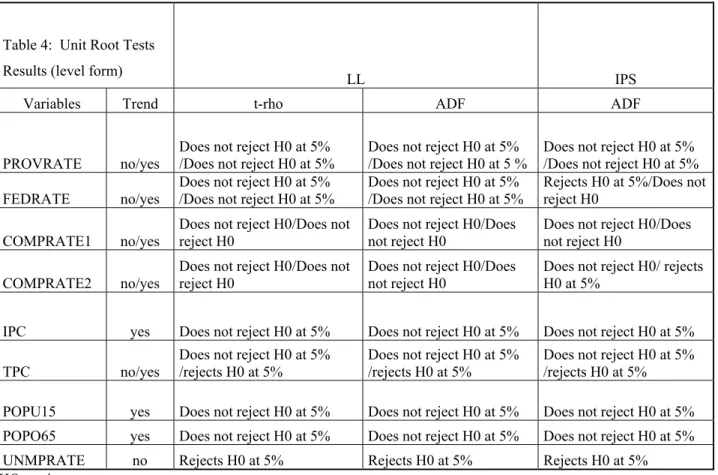
Table 4 reports the results for the LL test and IPS test for the variables considered in the model described in the last section.
Table 4: Unit Root Tests
Results (level form) LL IPS
Variables Trend t-rho ADF ADF
PROVRATE no/yes Does not reject H0 at 5% /Does not reject H0 at 5% Does not reject H0 at 5% /Does not reject H0 at 5 % Does not reject H0 at 5% /Does not reject H0 at 5% FEDRATE no/yes Does not reject H0 at 5% /Does not reject H0 at 5% Does not reject H0 at 5% /Does not reject H0 at 5% Rejects H0 at 5%/Does not reject H0 COMPRATE1 no/yes Does not reject H0/Does not reject H0 Does not reject H0/Does not reject H0 Does not reject H0/Does not reject H0 COMPRATE2 no/yes
Does not reject H0/Does not reject H0
Does not reject H0/Does not reject H0
Does not reject H0/ rejects H0 at 5%
IPC yes Does not reject H0 at 5% Does not reject H0 at 5% Does not reject H0 at 5% TPC no/yes Does not reject H0 at 5% /rejects H0 at 5% Does not reject H0 at 5% /rejects H0 at 5% Does not reject H0 at 5% /rejects H0 at 5% POPU15 yes Does not reject H0 at 5% Does not reject H0 at 5% Does not reject H0 at 5% POPO65 yes Does not reject H0 at 5% Does not reject H0 at 5% Does not reject H0 at 5% UNMPRATE no Rejects H0 at 5% Rejects H0 at 5% Rejects H0 at 5% HO : unit root
There is evidence that the dependent variable provincial tax rates is non-stationary, the null hypothesis cannot be rejected in the presence or not of a trend. The null hypothesis cannot be rejected for the federal tax rates or the competing tax rates. For the control variables, there is
evidence that the percentages of the population under 15 and over 65, the income per capita, and transfers per capita are non-stationary. However, as expected, the variable unemployment rate is stationary.
To correct this problem, one solution is to reconstruct the variables transforming them to obtain a stationary process. Two alternatives were tested in order to verify if the series could be transformed into a stationary process: the logarithmic form and the first difference. However, these transformations have also to be tested, as they will not necessarily lead the variables to become stationary. The results from the LL and IPS test for variables in their logarithmic and first difference forms are reported in tables 5 and 6.
Table 5: Unit Root Tests
Results (logarithmic form) LL IPS
Variables Trend t-rho ADF ADF
PROVRATE yes Rejects H0 at 10% Rejects H0 at 10% Rejects H0 at 10% FEDRATE yes Rejects H0 at 5% Rejects H0 at 10% Rejects H0 at 5% COMPRATE1 no Rejects H0 at 5% Rejects H0 at 5% Rejects H0 at 5% COMPRATE2 no Does not reject H0 Rejects H0 at 10% Rejects H0 at 5% IPC yes Does not reject H0 at 5% Does not reject H0 at 5% Does not reject H0 at 5% TPC no/yes Does not reject H0 at 5% /rejects H0 at 10% Does not reject H0 at 5% /rejects H0 at 10% Does not reject H0 at 5% /rejects H0 at 10% POPU15 yes Does not reject H0 at 5% Does not reject H0 at 5% Does not reject H0 at 5% POPO65 yes Does not reject H0 at 5% Does not reject H0 at 5% Does not reject H0 at 5% UNMPRATE no Rejects H0 at 5% Rejects H0 at 5% Rejects H0 at 5% H0: unit root
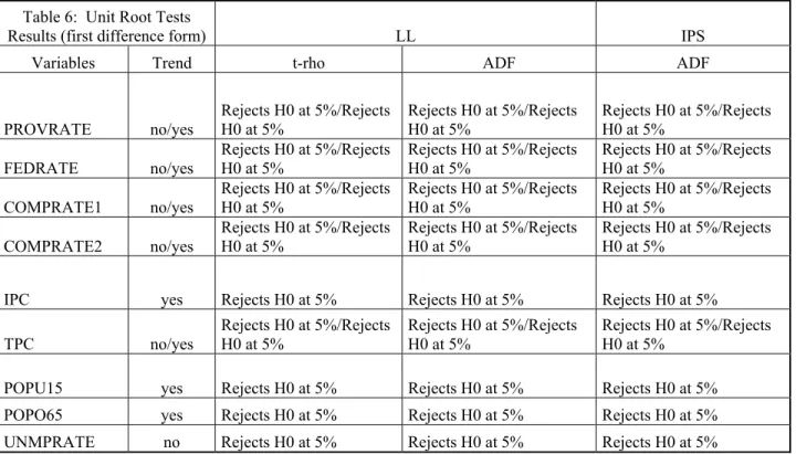
Table 6: Unit Root Tests
Results (first difference form) LL IPS
Variables Trend t-rho ADF ADF
PROVRATE no/yes Rejects H0 at 5%/Rejects H0 at 5% Rejects H0 at 5%/Rejects H0 at 5% Rejects H0 at 5%/Rejects H0 at 5%
FEDRATE no/yes Rejects H0 at 5%/Rejects H0 at 5% Rejects H0 at 5%/Rejects H0 at 5% Rejects H0 at 5%/Rejects H0 at 5% COMPRATE1 no/yes Rejects H0 at 5%/Rejects H0 at 5% Rejects H0 at 5%/Rejects H0 at 5% Rejects H0 at 5%/Rejects H0 at 5% COMPRATE2 no/yes
Rejects H0 at 5%/Rejects
H0 at 5% Rejects H0 at 5%/Rejects H0 at 5% Rejects H0 at 5%/Rejects H0 at 5% IPC yes Rejects H0 at 5% Rejects H0 at 5% Rejects H0 at 5% TPC no/yes Rejects H0 at 5%/Rejects H0 at 5% Rejects H0 at 5%/Rejects H0 at 5% Rejects H0 at 5%/Rejects H0 at 5% POPU15 yes Rejects H0 at 5% Rejects H0 at 5% Rejects H0 at 5% POPO65 yes Rejects H0 at 5% Rejects H0 at 5% Rejects H0 at 5% UNMPRATE no Rejects H0 at 5% Rejects H0 at 5% Rejects H0 at 5% H0: unit root
When taken in the logarithmic form, we can reject the hypothesis of unit root for the provincial tax rate, for the federal tax rate, the unemployment rate, and the transfers per capita. The results of the unit root tests are as expected; the null hypothesis of unit root can be rejected for all variables in their first difference.
A linear combination of non-stationary variables can be stationary and thus lead to spurious regression. “In the conventional time series case, cointegration refers to the idea that for a set of
variables that are individually integrated of order one, some linear combination of these variables can be described as stationary” (Pedroni, 1999, p.655). As we found evidence of the
majority of the variables being non-stationary, in the level form, it is useful to test for cointegration in order to estimate an alternative model. To test for the cointegration, the test developed by Pedroni (2004) was used. The null hypothesis of this test is no cointegration in dynamic panels with multiple regressors. According to Pedroni (2004), “an important feature of
these tests is that they allow not only the dynamics and fixed effects to differ across members of the panel, but also that they allow the cointegrating vector to differ across members under the alternative hypothesis”. The methodology developed by Pedroni (1999), gives us seven different
statistics: four are based on pooling along the within-dimension (referred as panel cointegration statistics) and three based on pooling along between-dimension (referred as group mean panel cointegration statistics). The first panel cointegration statistics is a type of non-parametric variance ratio statistic. The second is a panel version of a non-parametric statistic that is analogous to the Phillips and Perron rho-statistic. The third statistic is also non-parametric and is analogous to the Phillips and Perron t-statistic. Finally, the fourth of the simple panel cointegration statistics is a parametric statistic which is analogous to the augmented Dickey Fuller t-statistic. Concerning the group mean statistics, the first is analogous to the Phillips and Perron rho-statistic, the second is analogous to the Phillips and Perron t-statistic and the last one augmented Dickey-Fuller t-statistic (Pedroni, 2004).It is important to mention that “the
between-dimension-based statistics allow one to model an additional source of potential heterogeneity across individual members of the panel”. (Pedroni, 1999, p.658) This is a consequence of the
test’s construction: the between-dimension statistics allows for different autoregressive coefficients of the estimated residuals under the alternative hypothesis across different members. According to him, “Just as in the conventional time series case, each of these statistics is shown
to have a comparative advantage in terms of small sample size and power properties depending on the underlying data-generating process”. (Pedroni, 1999, p.658)
The cointegration relationship is tested taking all non-stationary variables and tests for cointegration. If the null hypothesis can be rejected, one variable is removed and then the test is rerun. The tests were made using a trend and time dummies. The results from the cointegration test for the level form of the variables are showed in the tables 7 and 8.
Table 7: Cointegration Tests Results (with competing tax rates criterion 1)
Variables Rejects H0 at 5% Does not reject H0 PROVRATE FEDRATE
COMPRATE1 IPC TPC POPU15 POPO65
panel stat; panel adf-stat;group pp-stat;group adf-stat;panel pp-stat;group
rho-stat panel v-stat
PROVRATE FEDRATE COMPRATE1 IPC TPC POPU15
panel rho-stat; panel pp-stat; panel adf-stat;
group pp-stat; group adf-stat; group rho-stat panel v-stat PROVRATE FEDRATE
COMPRATE1 IPC TPC panel rho-stat; group rho-stat panel v-stat;panel pp-stat; panel adf-stat; group pp-stat; group adf-stat; PROVRATE FEDRATE
COMPRATE1 IPC panel rho-stat
panel v-stat;panel pp-stat; panel adf-stat; group rho-adf-stat; group pp-adf-stat; group adf-stat;
HO: no cointegration
Table 8: Cointegration Tests Results (with competing tax rates criterion 2)
Variables Rejects H0 at 5% Does not reject H0 PROVRATE FEDRATE
COMPRATE2 IPC TPC POPU15 POPO65
panel stat; panel adf-stat;group pp-stat;group adf-stat;panel pp-stat;group
rho-stat panel v-stat
PROVRATE FEDRATE COMPRATE2 IPC TPC
POPU15 panel pp-stat; panel adf-stat; group pp-stat; group adf-stat; group rho-stat panel v-stat; panel rho-stat PROVRATE FEDRATE
COMPRATE2 IPC TPC panel adf-stat; group pp-stat; group adf-stat; panel rho-stat; panel pp-stat panel v-stat; PROVRATE FEDRATE
COMPRATE2 IPC panel pp-stat; panel adf-stat; group pp-stat; group adf-stat; group rho-stat panel v-stat; panel rho-stat PROVRATE FEDRATE
COMPRATE2 panel pp-stat; panel adf-stat; group pp-stat; group adf-stat panel v-stat; panel rho-stat; group rho-stat
PROVRATE FEDRATE panel pp-stat; panel adf-stat
panel v-stat; panel rho-stat; group rho-stat; group pp-stat; group adf-stat
H0: no cointegration
When using the criterion 1 for the competing tax rates, we find evidence of cointegration between the variables provincial tax rate, federal tax rate, competing tax rate, income per capita, transfers per capita, and population under 15. When considering the second criterion for the
competing tax rate, we also have evidence that all variables may have a linear combination that can be stationary, and thus lead to a spurious regression.
3.2 Fixed vs. Random effects model, heteroskedasticity, contemporaneous and serial correlation test
As a consequence of the results of the tests obtained in the last section, three models were estimated in to order to empirically determine the existence of vertical and horizontal externalities in the taxation of personal income in Canada. The first result that will be used is that all variables with exception of unemployment rate are non-stationary. Thus, the first model to be estimated will take all variables in their first differences, as this transforms them into stationary series process. The second model estimated takes the variables in their logarithmic form. The third model takes in consideration the cointegration between variables in their level form.
In this section we report the results of some test related to heteroskedasticity, contemporaneous and serial correlation to better adjust our estimations.13 Also, we report the Hausman tests done in order to decide between using fixed or random effects model. 14 Under the null hypothesis (difference in the coefficients are not systematic), we can conclude from the Hausman test that we have to use a fixed-effects model. For the heteroskedasticity test, a Breusch- Pagan test was used. The first step of this test is to estimate the model and then regress the square of the residuals on the independent variables. If we can reject the null hypothesis, we conclude the existence of heteroskedasticity. We also try to detect the type of heteroskedasticity using the xttest3 test in STATA. If we can reject the null hypothesis we conclude that there is inter-individual heteroskedasticity.
The results of the aforementioned test are reported in tables 9 and 10, according to the use of the different criteria for the calculation of the competing tax rates.
Level form First Difference form Logarithmic form Table 9: Tests
(competing tax rate 1) Result Conclusion Result Conclusion Result Conclusion Hausman test (fixed vs
random effects)
Rejects
H0 at 5% Fixed effects model
Does not reject H0
random effects model
Rejects H0
at 5% Fixed effects model Breusch-Pagan test for
Heteroskedasticity
H0: homoscedasticity Rejects H0 at 5% Heteroskedasticity Rejects H0 at 5% Heteroskedasticity Rejects H0 at 5% Heteroskedasticity inter-individual
heteroskedasticity H0:homoscedasticity inter-individual
Rejects
H0 at 5% inter-individual heteroskedasticity Rejects H0 at 5% inter-individual heteroskedasticity Rejects H0 at 5% inter-individual heteroskedasticity Contemporaneous correlation test (Breusch-Pagan) H0: no cross-sectional correlation Rejects
H0 at 5% Cross-sectional correlation Rejects H0 at 5% Cross-sectional correlation Rejects H0 at 5% Cross-sectional correlation Serial correlation test
(Wooldridge test) H0: no first-order correlation Rejects H0 at 5% Serial correlation Does not
reject H0 No serial correlation
Rejects H0
at 5% Serial correlation Level form First Difference form Logarithmic form Table 10: Tests
(competing tax rate 2) Result Conclusion Result Conclusion Result Conclusion Hausman test (fixed vs
random effects) Rejects at 5% Fixed-effects model Does not
reject H0 random effects model
Rejects H0
at 5% Fixed effects model Breusch-Pagan test for
Heteroskedasticity
H0: homoscedasticity Rejects H0 at 5% Heteroskedasticity Rejects H0 at 5% Heteroskedasticity Rejects H0 at 5% Heteroskedasticity inter-individual heteroskedasticity H0:homoscedasticity inter-individual Rejects H0 at 5% inter-individual heteroskedasticity Rejects H0 at 5% inter-individual heteroskedasticity Rejects H0 at 5% inter-individual heteroskedasticity Contemporaneous correlation test (Breusch-Pagan) H0: no cross-sectional correlation Rejects
H0 at 5% Cross-sectional correlation Rejects H0 at 5% Cross-sectional correlation Rejects H0 at 5% Cross-sectional correlation Serial correlation test
(Wooldridge test) H0: no first-order correlation Rejects H0 at 5% Serial correlation Does not
reject H0 No serial correlation
Rejects H0
The tests results are basically the same when using different criteria for the competing tax rates. The Hausman test allows deciding for a random effects model in the case where the variables are in their first difference form and for a fixed effects model where the variables are in the level form and in the logarithmic form. The two heteroskedasticity tests have for all cases the same result: we reject the null hypothesis and thus we should consider the existence of heteroskedasticity in our estimations. To correct for these potential problems, we use a Feasible Generalized Least Squares (FGLS) method for our regressions
3.3 Endogeneity
Another consideration in estimating the first difference form and the logarithmic form is the possible endogeneity of federal tax rates and competing tax rates. To deal with this problem we use these variables lagged by one period as an instrument (they are correlated with the contemporaneous value of the tax rates thus eliminating the correlation between the variables and the residuals of the original regression) and do the estimation in a two-stage instrumental variables method. Two tests were used to conclude whether or not we should use instrumental variables: the Hausman test and the Nakamura-Nakamura test. The null hypothesis of the Hausman test is that the difference between the two models estimated is not significant. Therefore, if we cannot reject the null hypothesis we can continue to estimate our model without instrumental variables. The Nakamura-Nakamura test is done in two steps: the first by regressing each endogenous variable on the instrumental variables and exogenous variables. The residuals of this estimation are now included in the original regression and if their coefficients are significant, we cannot reject the hypothesis of endogeneity of the variables tested. We tested three cases for each criterion for the calculation of the competing tax rates: one with the
except in the case of the variable one period lagged competing tax rate with the second criteria for the Hausman test, where we can reject the null hypothesis. But as the Nakamura-Nakamura test gave us the contrary result, we conclude that we should not use the potential instruments.
3.4 Regression Results
In light of the test results described in the last section, the three models that were estimated were a first difference model and the logarithmic model, using a Feasible Generalized Least Square method), and a DOLS (Dynamic Ordinary Least Square Method), also using a Feasible Generalized Least Square Method. The DOLS approach to estimate the model takes into account the cointegration results reported. The DOLS method was developed by Saikonen (1991). Using this method we do not have to take into account the problem of endogeneity, as asymptotically it has no effect on the robustness of the estimates. This method uses the leads and lags of the first difference of the variables that are non-stationary. Our choice of the numbers of leads and lags used here was one, due to our relatively small time sample. Table 11 reports the regression results obtained with the two different criteria used for the calculation of the competing tax rates and with the three different methods of estimation.
Table 11 : Regression Results
Variables Logarithmic form First difference form Level form (1 lead and 1 lag of the first difference) GLS (z-statistic) GLS (z-statistic) GLS (z-statistic) GLS (z-statistic) DOLS (z-statistic) DOLS (z-statistic) federal tax rate 0 .4421817*** 0.2434435*** 0.3095766*** 0.1672079*** 0.0975941 -0.0675773
(6.71) (4.42) (8.53) (5.80) (1.33) (-1.17)
competing tax rate 1 0.4172482*** - 0.4226955*** - 0.3279215*** -
(6.55) (6.13) (2.96)
competing tax rate 2 - 0.6501608*** - 0.7030242*** 0.5178079***
(13.77) (16.22) (8.33) equalization 0.0199227 0.0082379 0.000459 0.0003794 0.0025483 0.0035392** (0.92) (0.48) (1.17) (1.08) (1.49) (2.27) population under 15 -0.4990227*** -0.3753838*** 0.0023296 0.019554 -0.1565834*** -0.1718977*** (-3.80) (-3.54) (0.03) (0.30) (-3.24) (-4.74) population over 65 0.3054595*** 0.3571706*** 0.1015282 0.0157668 0.181354*** 0.1945079*** (4.34) (5.26) (0.71) (0.12) (3.74) (4.19) transfers per capita 0.0092915 -0.0001826 -5.70e-07 5.19e-07 1.75e-06 -1.71e-06**
(0.49) -(0.01) (-0.73) (0.82) (1.48) (-2.05)
income per capita -0.1699692*** -0.1809006*** -1.40e-06*** -1.10e-06*** -3.99e-07 -4.41e-07*
The three different estimations give us more confidence regarding the existence of vertical and horizontal externalities and the impact of if equalization grants on the provincial tax rates. The logarithmic model makes our interpretations easier, as the coefficients are elasticities. The first difference model is harder to interpret though, as we have to consider how the temporal change in the independent variable influences the same kind of change in the dependent variable. But this does not prevent us from at least achieving some conclusions about what kind of reaction the provinces have given changes in the federal tax rate and other provincial tax rates. The DOLS method is certainly the easiest model to interpret as we take the variables in their level form.
3.4.1 Vertical Tax Interaction and Vertical Externalities
The three different estimations of the impact of the federal tax rate on the provincial tax rate show evidence of the existence of vertical externalities. The estimation of our model in the logarithmic form and in the first difference form allows us to conclude that the provinces have a positive reaction to the federal tax rate, regardless of the method of calculation of the competing tax rates. But the impact is slightly different: using the competing tax rate 1, the magnitude of the impact is smaller than the one obtained from the competing tax rate 2. However, using the DOLS method, the conclusion is not the same and even ambiguous. The two different ways of calculating the competing tax rates show us different signs for the federal tax rate, and we cannot make any conclusions as the coefficients are not significant.
The positive sign of the federal tax rate is similar with the empirical results found in other studies of taxation of personal income. Both Esteller-Moré and Solé-Ollé (2001) and Esteller-Moré and Solé-Ollé (2002) found this result for the United States and Canada. The result is, however, the opposite of the one found in the Goodspeed (2000) for the OCDE countries. Besley and Rosen (1998) and Hayashi and Boadway (2001), found also a negative sign of the federal tax rate in the cases of taxation of cigarettes and gasoline in the United States and business income in Canada, respectively. However, it is hard to compare the taxation of personal income and the taxation of
From the theoretical point of view, as pointed out in section I, the effect of the changes in the federal rate on provincial tax rates is ambiguous, and we are only able to determine these signs empirically. Our results from the first difference model and from the logarithmic form model indicate that if federal tax rate increases, the revenue of provinces decreases and so to set the same level of public goods as before, the province will have to increase its taxes rates. Also, we have evidence from our estimations that the marginal cost of public funds decreases as the federal tax rate increases, leading to a positive effect on the provincial tax rate. We conclude also that due to these vertical externalities, the provincial tax rate set in a way that is higher than what would be optimal from a social point of view.
3.4.2 Horizontal Tax Interaction and Horizontal Externalities
The horizontal interaction is much more apparent in our results as all our estimations reveal a significant and positive coefficient of the variable competing tax rate for both criteria. Our results coincide with the ones found for the taxation of business income in Canada by Hayashi and Boadway (2001) and for the taxation of personal income in the United States and Canada by Esteller-Moré and Solé-Ollé (2001) and Esteller-Moré and Solé-Ollé (2002). Also, we find that using the criterion to calculate the competing tax rate based on Esteller-Moré and Solé-Ollé (2002) the coefficients of the competing tax rate are larger than the ones estimated with the GDP criterion. We can deduce from the theoretical model and from our estimations that even if the marginal benefit of public goods decreases in province i followed by the increase of the tax rate of province j (as we have inflow of tax base to province i we may not have a decrease in province i s tax rate. This may be explained by the uncertain effect on the marginal cost of public funds. However, as we find positive coefficients for the competing provincial tax rate, the effect of the decrease in the marginal cost of public funds in province i seems to offset the effect of the
(2002) found a positive and significant relation between equalization grants and provincial personal income tax rates. Smart (2007) also finds a positive and significant effect of equalization grants in tax rates. However, our estimates do not allow us to reach such a conclusion. Actually, the coefficients of the dummy variable equalization are all positive and their magnitudes are very small, but none of them, with exception of the DOLS estimation with the competing tax rate 2, were significant.
3.4.4 Control Variables
Three of our control variables were significant: population under 15, population over 65, and income per capita. The coefficient of the variable income per capita is negative; richer populations have lower taxation. The population over 65 has a positive sign, in contrast with the variable population under 15, which has a negative sign. The unemployment rate has a positive sign in all cases, but is not significant. Finally, we surprisingly did not find evidence that the transfers per capita have an influence on provincial tax rates, at least not contemporaneously. These results are different than the ones obtained by Esteller-Moré and Solé-Ollé (2002). However, comparing the coefficients of the control variables of our estimations may not be useful in this case, as their model presents different specifications.
CONCLUSIONS
The purpose of this paper was to investigate empirically vertical and horizontal tax interaction in a federation as a consequence of the taxation of the same tax base. We showed in section I that the sign of such interactions can only be determined empirically. In order to test empirically theses fiscal interactions, we calculated the effective provincial and federal personal income tax rates. We calculated the competing tax rates using two different criteria and used a dummy variable for equalization grants was included in an attempt to establish if this particularity of the Canadian system influences the provincial tax rates. In particular, our research differs from the other studies of tax interaction as we considered the possibility of non-stationary and cointegrated series in the context of panel data.
The results of our estimations confirm tax interaction and the presence of both vertical and horizontal externalities. We have evidence of a positive reaction by provinces given an increase in the federal tax rates. However, we could not reach this conclusion from the DOLS estimation. The results also suggest that the provincial rates are positively affected by the changes in competing tax rates, even using different criteria for calculating the competing tax rates. The signs of our estimations for the federal tax rates and provincial tax rates coincide with the studies regarding the taxation of personal income done by Esteller-Moré and Solé-Ollé (2001) and Esteller-Moré and Solé-Ollé (2002). It would be interesting to extend the model to consider more periods and particularly to use statutory tax rates as opposed to effective rates.
Regarding the equalization grants, we could not affirm that it has an influence on the province’s tax decisions. This result was not expected, as other studies showed positive reaction of
REFERENCES
Besley, T.J., Case, A. (1995), "Incumbent Behaviour: Vote Seeking, Tax Setting and Yardstick Competition", American Economic Review, 85 (1), 25-45.
Besley, T.J., Rosen, H.S. (1998). "Vertical externalities in tax setting: evidence from gasoline and cigarettes". Journal of Public Economics, 70 (3), 383–398.
Boadway, R.W., Wildasin, D.E. (1984). Public Sector Economics, Little, Brown, Toronto; second edition.
Canadian Tax Foundation (1981-2005), Finances of the Nation, Toronto.
Department of Finance, Canada, http://www.fin.gc.ca/toce/2000/jul-e.html.
Doak, J. (1990). “The Relationship between Federal and Provincial Income Tax Rates in Canada Since 1965.”Canadian Tax Journal, 38 (5), 1227–1235.
Esteller-Moré, A., Solé-Ollé, A. (2002), “Tax Setting in a Federal System: The Case of Personal Income Taxation in Canada.” International Tax and Public Finance, 9 (3), 235-257.
Esteller-Moré, A., Solé-Ollé, A. (2001). "Vertical income tax externalities and fiscal interdependence: evidence from the US." Regional Science and Urban Economics 31(2-3):,247-272.
Feldstein, M. and G. Metcalf. (1987).“The Effect of Federal Tax Deductibility on State and Local Taxes and Spending.” Journal of Political Economy, 95 (4), 710-36.
Goodspeed, T. J. (2000), “Tax Structure in a Federation”, Journal of Public Economics, 75 (3), 493–506.
Hayashi, M., R. Boadway. (2001). “An Empirical Analysis of Intergovernmental Tax Interaction: The Case of Business Income Taxes in Canada.” Canadian Journal of Economics, 34 (2), 481– 503.
Im, K.S, Pesaran, M.H., Shin Y., “Testing for unit root in heterogenous Panels” Journal of
Econometrics, 115(1),53-74.
Levin, A., C. F. Lin, et al. (2002). "Unit root tests in panel data: asymptotic and finite-sample properties." Journal of Econometrics,108, 1-24.
MacNevin (2004). Canadian Tax Foundation, Canadian Tax Paper 109: The Canadian
Federal-Provincial Equalization Regime: An Assessment.
Pedroni, P. (1999). "Critical Values for Cointegration Tests in Heterogeneous Panels with multiple Regressors." Oxford Bulletin of Economics and Statistics, 61, 653-670.
Pedroni, P. (2004), “Panel Cointegration: Asymptotic and Finite Sample Properties of Pooled Time Series Tests With an Application to the PPP hypothesis”, Econometric Theory, 20, 597-625
Saikkonen, P. (1991). "Asymptotically Efficient Estimation of Cointegration Regressions."
Econometric Theory 7(1), 1-21.
Smart, M. (1998). “Taxation incentives and deadweight loss in a system of intergovernmental transfers”, Canadian Journal of Economics, 31,189-206.