HAL Id: hal-01053180
https://hal.archives-ouvertes.fr/hal-01053180
Submitted on 5 Aug 2014
HAL is a multi-disciplinary open access
archive for the deposit and dissemination of
sci-entific research documents, whether they are
pub-lished or not. The documents may come from
teaching and research institutions in France or
abroad, or from public or private research centers.
L’archive ouverte pluridisciplinaire HAL, est
destinée au dépôt et à la diffusion de documents
scientifiques de niveau recherche, publiés ou non,
émanant des établissements d’enseignement et de
recherche français ou étrangers, des laboratoires
publics ou privés.
Unilateral Constraints on the Position
Oscar Eduardo Montaño Godinez, Yuri Orlov, Yannick Aoustin
To cite this version:
Oscar Eduardo Montaño Godinez, Yuri Orlov, Yannick Aoustin. Nonlinear H_inf -Control of
Mechan-ical Systems under Unilateral Constraints on the Position. Congreso Nacional de Control Automático
AMCA 2013, Oct 2013, Ensenada, Baja California, Mexico. pp.1-6. �hal-01053180�
Abstract— The work focuses on the study of hybrid
mechanical systems under unilateral constraints on the position. The problem of robust control of mechanical systems is addressed under unilateral constraints by designing a nonlinear -controller developed in the nonsmooth setting, covering impact phenomena. Performance issues of the nonlinear -tracking controller are illustrated in a numerical simulation
Keywords: hybrid systems, robust control, nonlinear control, tracking, mechanical systems.
I. INTRODUCTION
The study of hybrid dynamical systems has recently attracted a significant research interest, basically, due to the wide variety of applications and the complexity that arises from the analysis of this type of systems. See, e.g., the relevant surveys by Goebel, Sanfelice and Teel (2009), Savkin and Evans (2002) and Antsaklis (2000).
Description of hybrid systems involve both continuous-valued and discrete-continuous-valued variables. Their evolution is given by equations of motion that generally depend on both variables. In turn, these equations contain mixtures of logic and discrete-valued or digital dynamics and continuous-variable or analog dynamics. The continuous and discrete dynamics interact at “event” or “trigger” times when the continuous state hits certain prescribed sets in the continuous state space (Branicky, Borkar & Mitter, 1998).
The focus of this work is centered on the study of a subclass of hybrid systems, namely, the autonomous-impulse hybrid systems, also recognized as dynamical systems under unilateral constraints (Brogliato, 1996).
More precisely, mechanical systems of the general form = Φ , + Ψ , , ≥ 0 are under study, where ∈ is the vector of generalized coordinates of the system; ∈ is the vector of inputs (or controllers) that generally involves a state feedback loop; and the function ⋅,⋅ represents a unilateral constraint that is imposed on the state (specifically, the position). A general property of these systems is that their solution is nonsmooth, which arises from the occurrence of impacts when trajectories attain the surface , = 0. Some authors such as Neši , Zaccarian and Teel (2008), Haddad et al. (2005), Orlov and Acho (2001) and Nguang and Shi (2000) to name a few have addressed the disturbance attenuation problem for hybrid
dynamical systems. Typically, a pair of Riccati equations, coming from continuous and discrete dynamics, are separately involved and strict conditions are thus imposed on their solutions to simultaneously satisfy both equations. Apart from this, an unrealistic use of an impulsive control is admitted at the impact times.
Motivated by the fact that impulsive inputs, applied at the impact time instants, cause the well-posedness problem of defining dynamics of such a system (Brogliato, 1996), and they are in addition hardly possible to be physically implemented, this work intends to introduce a new control strategy that avoids using impulsive control inputs while ensuring asymptotical stability for the undisturbed system, and at the same time, possessing the ℒ -gain of the disturbed system to be less than an appropriate disturbance attenuation level . An essential feature, adding the value to the present investigation, is that not only standard external disturbances are in play but also their discrete-time counterpart, typically ignored in the existing literature, that occurs due to imperfect knowledge of the restitution rule at the impact time instants.
II. PROBLEM STATEMENT
Consider the nonlinear system (1)-(4)
= , + , + , , ≠ , ! ≥ 0 (1) ! " #∇ % &! ' = −)! * #∇% &! ' + + , = , &! ' = 0 (2) , = ℎ , + . , , ≠ , ! ≥ 0 (3) ,+= −)! * #∇% &! ' + +, = , &! ' = 0, . = 1,2, … (4) with the functions , , , ℎ, . , of appropriate dimensions which are piece-wise continuous in and twice continuously differentiable in .
For the above class of nonlinear system, ∈ ℝ represents the state vector, consisting of = 4!, !5#, where ! ∈ ℝ and ! ∈ ℝ ; ∈ ℝ the control input of the same dimension as ! (thus confining investigation to the fully actuated case), and ∈ ℝ6 collects exogenous signals affecting the system. Inequality ! ≥ 0 (with ! ∈ ℝ7)
Nonlinear
-control of mechanical systems under unilateral
constraints on the position
O.E. Montaño
1,*, Y. Orlov
1,, Y. Aoustin
2,1Department of Electronics and Telecommunications, Center for Scientific Research and Higher Education at
Ensenada, Baja California, P.O. BOX 434944, San Diego, CA 92143-4944, USA
2L'UNAM, Institut de Recherche en Communications et Cybernétique de Nantes, \UMR CNRS 6597, \CNRS,
École Centrale de Nantes, Université de Nantes, 1, rue de la Noë, BP 92101. 44321 Nantes, Cedex 3, France
stands for the set of unilateral constraints, i.e., the subspace Φ ⊂ ℝ within which the system evolves. The restitution law, given by equation (2), establishes the interaction between the continuous dynamics (1) and the surface ! = 0, reached at = ; ) ∈ 40,15 is the restitution coefficient, whereas +∈ ℝ9 is a perturbation accounting for inadequacies of the restitution law. For making physical sense of the energy dissipation, it is assumed that
− 1 − ) ! :* #∇% &! : ' < +< )! :* #∇% &! : ' (5)
Equations (1) and (3) describe the continuous dynamics before the system hits the reset surface ! = 0, and equations (2) and (4) govern the way that the states are instantaneously changed when the resetting surface is hit. This model is restricted to surfaces of co-dimension one. Under certain assumptions (Brogliato, Nicolescu and Orhant, 1997), this restriction can be relaxed to surfaces of higher co-dimensions.
The ℋ -control problem consists in finding a controller, if any, such that the undisturbed, closed-loop system (1)-(4) is asymptotically stable, and such that the ℒ -gain of the disturbed system is less than , that is the inequality
holds with some positive definite functions =: , > = 0, … , ? for all @ > 0 and ? ∈ ℤ such that C≤ @. This
definition is consistent with the notion of dissipativity introduced by Willems (1972) and Hill & Moyan (1980), that has become standard in the literature, and represents a natural extension for hybrid systems (see, e.g., the works by Neši , Zaccarian & Teel (2008), Yuliar, James & Helton (1998), Lin & Byrnes (1996) and Baras & James (1993)).
III. NONLINEAR ℋ -CONTROL SYNTHESIS
A. Global state-space solution
The main result of the present work is given below.
Theorem 1. Suppose that in a domain ∈ EF, ∈ ℝ there is a Lipchitz continuous, positive definite, decrescent functionG , , a positive definite function H and a constant > 0 such that for the system (1)-(4) with assumptions above and the initial conditions withinEF, the following conditions C1. G :" , : < G :* , : , > = 1, … , ? provided that += 0 C2. IJIK+IJI , + , L + , L + ℎ#ℎ + L #L − L #L ≤ −H hold under L = MN # , OIJI P # , L = − # , OIJ I P # .
Then driven by the controller
= L , , (7)
the closed-loop undisturbed system (1)-(4) is asymptotically stable, while its disturbed version possesses a ℒ -gain less than . If in addition, G , is radially unbounded, then the result becomes global.
Proof. The proof is brought up into two parts. First we demonstrate that the inequality
QR, R d # KT ≤ UQR R d # KT V + W =′:& : ' C :YZ (8) holds for all @ > 0 and ? ∈ ℤ such that C≤ @, and some positive definite functions =′:& : ', > = 0, … , ?. Suppose there is a positive definite function G , such that
G @ , @ + W G :* , : C :Y − W G :" , : C :YZ ≤ − QR, R d # KT + QR R d # KT (9)
holds. Then inequality (8) is achieved by setting
=′:& : ' = G :" , : , > = 0 … ?. (10)
In order to validate inequality (9) let us represent it in the equivalent differential form
dG
d ≤ −,#, + # , ∈ :, :" (11)
between impact instants :, > = 1, … , ?. Then for the undisturbed system, G , can be used as a Lyapunov function. Indeed, along the trajectories of such a system, we have dG d ≤ −,#, (12) and G :" , : < G :* , : (13)
provided that C1 and C2 are satisfied. Just in case, inequalities (12)-(13), coupled to the assumption that G , is decrescent, ensure that lim:→ G :" , : = 0. The undisturbed system is thus asymptotically stable (Theorem 3.7, Orlov, 2009) and in addition, it is globally asymptotically stable if G , is radially unbounded.
For the disturbed system, we verify (11) and (13) independently. For the continuous dynamics, the inequality
_G
_ +_G_ , + , + , + ℎ#ℎ
+ # − # ≤ −H (14)
is guaranteed by condition C2. To reproduce this conclusion, let us define the Hamiltonian function
`a , , , =IJIK+IJI , + , +
, + ℎ#ℎ + # − # (15)
Then solving the equations QR, R d # KT + WR,+ : R C :Y ≤ UQR R d # KT + WR + : R C :Y V + W =:& :* ' C :YZ (6)
_`a _ bc,d Y ef,eN = 0, _`a _ bc,d Y ef,eN = 0 , we obtain L = MN # , OIJI P#, L = − # , OIJI P#. Since `a , , , is quadratic in , its Taylor
expansion around = L , = L is expressed as `a , , , = `a , L , L , + R − L R
− R − L R (16)
Thus, taking into account condition C2, we obtain
`a , L , L , ≤ −H (17)
and combining the result with (15)-(16) yields inequality (14) that in turn ensures (9).
The second part of the proof consists of demonstrating that the inequality
WR,+ : R C :Y ≤ gWR + : R C :Y h + Wi=":& :* 'i C :Y (18)
holds for ? such that C≤ @, and some positive definite functions =": ⋅ , > = 1, … , ?. Clearly, it suffices to prove its simplified version
R,+ : R ≤ R + : R + i=">& :* 'i (19)
for a single impact and all > ∈ 41, ?5. Substituting (4) in (19) and applying the Cauchy-Schwartz and triangle inequalities to the left side, we obtain
2) i! :* #∇k & : 'i + 2R + : R
≤ R + : R + i=":& >− 'i .
(20) By setting=">&! :* ' = 2! :* #∇% &! : ', then
inequality (18) is achieved for ≥ 2. Combining this result with (10), we establish the dissipativity inequality (5) with
=:& : '
= lG G Z , Z , > = 0
:" , : + 2! :* #∇% &! : ', > = 1, … , ?
(21) This completes the proof. ∎
B. Local state-space solution
The subsequent local analysis involves the linear ℋ -control problem for the system
= n + E + E , ≠ , ! ≥ 0 (22) ! " #∇ % &! ' = −)! * #∇% &! ' + +, = , &! ' = 0 (23) , = o + p , ≠ , ! ≥ 0 (24) ,+= −)! * #∇% &! ' + +, = , &! ' = 0 (25) ∀. ∈ ℤ", where n =Ir I sYZ, E = 0, , E = 0, , o =ItI sYZ, p = . 0, .
Theorem 2. Given the system linearization (22)-(25) and
some 0 < u < uZ, then conditions C1-C2 hold locally around the equilibrium = 0 of the nonlinear system (1)-(4) with
G , = #vw (26)
H =u2 R R (27)
and the state feedback
= − , #v
w , (28)
is a local solution of the ℋ -control problem for the nonlinear system (1)-(4) provided that vw is a bounded, symmetrical, positive definite solution of the differential Riccati equation
−vw = vw n + n# vw + o# o
+ vw x1E E#− E E#y vw + uz. (29)
Proof. It should be noted that the time-varying strict bounded real lemma (Orlov, Acho & Solis, 1999) yields a constructive tool of verifying the existence of an appropriate solution of the differential Riccati equation (29). Recall that in accordance with this lemma, once the equation (30)
−v = v n + n# v + o# o
+ v x1 E E#− E E#y v (30)
possesses a symmetrical, positive semidefinite solution v then there exists a positive constant uZ such that the perturbed Riccati equation (29) has a unique bounded, positive definite symmetric solution vw for each u ∈
0, uZ .
It should also be noted that by setting G , = #v the Hamilton-Jacobi-Isaacs inequality (17) subject to H = 0 degenerates to the differential Riccati equation (30).
Thus, employing (29), we can set G , = #vw to locally meet the Hamilton-Jacobi-Isaacs inequality (17) with the positive definite function H = −wR R . Finally, applying Theorem 1 to (22)-(25) subject to (26), (27), (29), the controller (28) is a local solution to the ℋ -control problem. This completes the proof. ∎
Remark 1. For autonomous systems, where all functions in
(1)-(4) and (22)-(25) are time-independent, the differential Riccati equations (30) and (29) degenerate to algebraic Riccati equations (ARE) by setting vw = 0 and v = 0.
C. Application to mechanical systems subject to unilateral constraints
In this section, the Lagrange model for mechanical manipulators will be used, in order to follow a trajectory composed of free-motion phases separated by transition phases, as follows:
Free-motion phase:
{ + o , + H = | + (31)
Transition phases:
" = * (33)
" #∇k & ' = −) * #∇k & ' + + (34)
& ' = 0 (35)
where ∈ ℝ is a position, | ∈ ℝ is a control input, ∈ ℝ is an external disturbance, + is a perturbation due
to the modeling of the restitution rule (34), { , o , , H are matrix functions of the appropriate dimensions. From the physical point of view, is the vector of generalized coordinates, | is the vector of external torques, { is the inertia matrix, symmetric and positive definite for all ∈ ℝ , o , is the vector of Coriolis, centrifugal torques and viscous friction and H is the vector of gravitational torques. As a matter of fact, the functions{ , o , , H are smooth functions of their arguments.
Remark 2: Notice that equations (31)-(35) do not provide
a control action during the transition phase, mainly because such a control action would be impulsive in nature, whose implementation is challenging in practice.
Remark 3: In this fully-actuated case, it is clear that the
aim of the robotic task is to follow a desired time-varying trajectory that will bounce in the surface = 0 at some instants = , . = 1,2, …. An extension to the plant stabilization constrained to the surface = 0 is under study.
Now, suppose that there exists a discontinuous periodic solution = + of the undisturbed system (31)-(35), driven by an input torque | = |+. In other words, suppose that there exis initial conditions of (31)-(35) with = += 0, | = |+, such that it exhibits a periodic solution. Then, our
objective is to design a controller of the form
| = |++ (36)
|+= { + ++ o +, + ++ H + (37)
that imposes on the disturbance-free manipulator motion desired stability properties around + while also locally attenuating the effect of the disturbances. Thus, the controller to be constructed consists in the trajectory feedforward compensator design (37) and a disturbance attenuator synthesis , internally stabilizing the closed-loop system around the desired trajectory.
We confine our research to the position tracking control problem where the output to be controlled is given by
, = U}~ +0− }• +− V + g10 0h (38) ,+= −) * #∇k & ' + + (39)
with positive weight coefficients }~, }•.
The ℋ position tracking control problem for robot manipulators subject to unilateral constraints on the position can formally be stated as follows. Given a mechanical system (31)-(35) a desired trajectory + to track, and a
real number > 0, it is required to find (if any) a state feedback controller such that the undisturbed closed-loop system is uniformly asymptotically stable around + and its ℒ -gain is locally less than , for all @ and all piecewise continuous functions , + for which the state trajectory of the closed-loop system starting in a neighborhood of the initial point & 0 , 0 ' = & + 0 , + 0 ' remains in a neighborhood of the desired
trajectory + for all ∈ 40, @5.
In order to accomplish this task, the following assumptions are made:
+ ∈ = 0, k=1,2,… (40)
+: ≠ 0, > = 1, … , € for almost all . (41)
To begin with, let us introduce the state deviation vector = ! , ! # where ! = + − is the position
deviation from the desired trajectory + , and ! =
+ − is the velocity deviation from the desired
velocity .
After that, let us rewrite the state equations (31)-(35), (38)-(39) in terms of these deviations:
Free-motion phase errors:
! = ! (42) ! = ++ {* +− ! 4o +− ! , +− ! + − ! + H +− ! + { + + − o +, + +− H + − − 5 (43) ! ≥ 0 (44) , = g}~0! }•! h + g10 0h . (45)
Transition phase errors:
! " = ! * (46)
! " #∇
%f &! ' = −)! * #∇%f &! ' + + (47)
&! ' = 0 (48)
,+= −)! * #∇%f &! ' + + (49)
The above ℋ -tracking control problem can be specified as follows: , = x ! ++ {* +− ! 4o +− ! , +− ! − ! 5y + x{* 0 +− ! 4H +− ! − { + +5y + x{* +− ! 4−o0+, + +− H + 5y, (50) , = x−{* 0+− ! y, (51) , = x−{* 0+− ! y (52) ℎ = g}~0! }•! h (53) . = g10 0h (54)
Theorem 3. Let the following conditions be satisfied 1) (40) and (41) hold for the desired trajectory to
follow
2) There exists a symmetrical, positive definite solution vw to (29), where n, E , E , o are obtained by the linearization of (50)-(54), under someu > 0.
Then, the state feedback
= − # , v
w (55)
is a local solution of the ℋ -position tracking problem for the mechanical manipulator under unilateral constraints on the position (31)-(35).
Proof. By applying Theorem 2 to the error system (42)-(54) specified with a given trajectory subject to (40)-(41) the validity of the theorem is established. ∎
IV. NUMERICAL SIMULATION
A. Mass-spring-damper-barrier model
Theorem 3 will be applied to a simple mass-spring-damper-barrier system as depicted in figure 1, where ‡ represents the mass, . the spring constant, ˆ a damping constant, | is the applied control force, and represents the position. The objective is to follow a trajectory that bounces against the wall located at = 0.
Figure 1. Mass-spring-damper-barrier system For the free-motion dynamics ( > 0 , the model is:
‡ + ˆ + . = | +
= , =
=
= −‡ −. ‡ +ˆ ‡ | +1 ‡1 whereas for the transition phase ( = 0 :
"= * "= −) *+ + + " = + * + " = −) + *
The notation " ( *) is equivalent to " ( * ). The variables and + were introduced to account for model inadequacies, and non-modeled external forces, such as friction. Now, let’s define the error variables ! = − + and! = − +. Rewriting the system with these error variables, leads to the free-motion phase error system:
| = ‡ ++ . ++ ˆ ++ = g−0. 1 ‡ −‡ˆh ‰ŠŠŠ‹ŠŠŠŒ • + g01 ‡h Ž •f + g01 ‡h Ž •N , = U}0 0~ 0 0 }• V ‰ŠŠ‹ŠŠŒ • + g10 0h ‘ ’fN
And to the transition phase error equations:
"= “1 0
0 −)” *+ “01” +
,+= −)!*+ +
From the expressions above, we can identify the terms n, E , E , o, necessary to solve (29) (see remark 1).
B. Simulation results
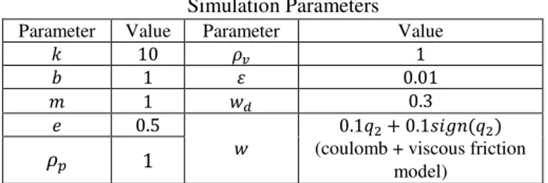
The simulation shown in figure 2 was performed using Matlab and the parameters from table 1. The solution of (30) was obtained by iterating on , and the infimal achievable level attained was ∗≈ 0.73. From theorem 1, it is known that ≥ ™2; however, = 2 was selected to avoid an undesirable high-gain controller design that would appear for a value of close to the optimum. With = 2, the value of u = 0.01 was obtained so the corresponding perturbed Riccati equation (29) has a positive definite solution.
TABLE I Simulation Parameters
Parameter Value Parameter Value
. 10 }• 1
ˆ 1 u 0.01
‡ 1 + 0.3
) 0.5 0.1 + 0.1›> €
(coulomb + viscous friction model)
}~ 1
The trajectory to follow was generated by a Van der Pol oscillator bouncing against a surface with a restitution coefficient of 0.5. The model used was:
Free-motion phase (! < 0 : ! = œ œ = •(1 − ! )œ − ! Transition phase (! = 0): !( ") = !( *) œ( ") = −)œ( *)
The parameters used for this oscillator were • = 1, ) = 0.5, !(0) = 0 and œ(0) = 1.0126. This reference system generates a hybrid periodic orbit (Grizzle et al., 1999). Thus, the planned trajectory to follow by the system will be:
+( ) = !( ), +( ) = œ( )
From figure 2 we can see that the system tracks the desired trajectory in a sound manner despite the disturbances affecting the free-motion (friction) and transition phases (deviation from restitution coefficient), while asymptotically stabilizing the error for the undisturbed system.
‡
. |
From figure 3 we can conclude that as the parameter approaches the limit value = ™2, the system begin to decrease its disturbance attenuation property. For values of less than this limit value, this property is lost, as predicted.
Undisturbed system Disturbed system
Figure 2. Trajectory tracking for = 2. Left: undisturbed system. Right: disturbed system.
= 10 = 5
= 2 = 1.45
Figure 3. Behavior of the system’s ℒ -gain while varying the parameter .
V. CONCLUSIONS
In this paper, the state feedback ℋ -control is solved for mechanical systems subject to unilateral constraints on the position. A global (local) solution for the tracking problem is found by solving only a unique Hamilton-Jacobi-Isaacs inequality (or differential Riccati equation for finding a local solution), which represents an advantage over solutions available in the existing literature. Effectiveness of the proposed disturbance attenuation design has been supported
by the numerical simulations, made for a mass-spring-damper-barrier model operating in the presence of a coulomb friction force under an uncertain restitution coefficient.
REFERENCES
Antsaklis, P. J. (2000). A brief introduction to the theory and applications of hybrid systems.In Proc IEEE, Special Issue on Hybrid Systems: Theory and Applications.
Baras, J.S. & James, M.R. (1993). Robust output feedback control for discrete-time nonlinear systems: the finite-time case. Proceedings of the 32nd IEEE Conference on Decision and Control, 55(1), 15-17. Branicky, M. S., Borkar, V. S., & Mitter, S. K. (1998). A unified framework
for hybrid control: Model and optimal control theory. Automatic Control, IEEE Transactions on, 43(1), 31-45.
Brogliato, B. (1996). Nonsmooth mechanics: models, dynamics, and control. Springer Verlag.
Brogliato, B., Niculescu, S. I., & Orhant, P. (1997). On the control of
finite-dimensional mechanical systems with unilateral
constraints. Automatic Control, IEEE Transactions on, 42(2), 200-215.
Goebel, R., Sanfelice, R. G., & Teel, A. (2009).Hybrid dynamical systems.Control Systems, IEEE, 29(2), 28-93
Grizzle, J. W., Plestan, F., & Abba, G. (1999). Poincare's method for systems with impulse effects: application to mechanical biped locomotion. In Decision and Control, 1999. Proceedings of the 38th IEEE Conference on (Vol. 4, pp. 3869-3876). IEEE.
Haddad, W. M., Kablar, N. A., Chellaboina, V., & Nersesov, S. G. (2005). Optimal disturbance rejection control for nonlinear impulsive dynamical systems. Nonlinear Analysis: Theory, Methods & Applications, 62(8), 1466-1489.
Hill, D., & Moylan, P. (1980). Connections between finite-gain and asymptotic stability. Automatic Control, IEEE Transactions on, 25(5), 931-936.
Lin, W., & Byrnes, C. I. (1996). ℋ -control of discrete-time nonlinear systems. Automatic Control, IEEE Transactions on, 41(4), 494-510. Neši , D., Zaccarian, L., & Teel, A. R. (2008). Stability properties of reset
systems. Automatica, 44(8), 2019-2026.
Nguang, S. K., & Shi, P. (2000). Nonlinear ℋ filtering of sampled-data systems. Automatica, 36(2), 303-310.
Orlov, Y. V. (2009). Discontinuous systems: Lyapunov analysis and robust synthesis under uncertainty conditions. Springer.
Orlov, Y., & Acho, L. (2001). Nonlinearℋ -control of time-varying systems: a unified distribution-based formalism for continuous and sampled-data measurement feedback design. Automatic Control, IEEE Transactions on,46(4), 638-643.
Orlov, Y., Acho, L. & Solis V. (1999). Nonlinear ℋ -control of time-varying systems. Decision and Control, Proceedings of the 38th IEEE Conference on. IEEE, p. 3764-3769.
Savkin, A. V., & Evans, R. J. (2002).Hybrid dynamical systems: controller and sensor switching problems. Birkhauser.
Willems, J. C. (1972). Dissipative dynamical systems part I: General theory.Archive for rational mechanics and analysis, 45(5), 321-351. Yuliar, S., James, M. R., & Helton, J. W. (1998). Dissipative control
systems synthesis with full state feedback. Mathematics of Control, Signals and Systems, 11(4), 335-356.
0 5 0 0.5 1 1.5 2 t [sec] q [ c m ] 0 5 -0.5 0 0.5 t [sec] x 1 = q 1 -q 1 d [ c m ] 0 5 0 0.5 1 1.5 2 t [se q [ c m ] 0 5 -0.5 0 0.5 t [se x 1 = q 1 -q 1 d [ c m ] 0 5 0 5 10 15 20 t [sec] 0 5 0 1 2 3 4 5 t [sec] 0 5 0 0.2 0.4 0.6 0.8 1 1.2 t [sec] 0 5 0 0.2 0.4 0.6 0.8 1 1.2 t [sec] zTz dt + Σ z d Tz d γ2 wTw dt + γ2Σ wdTwd + Σβ(x-)